Fast Parameter Identification of the Fractional-Order Creep Model

Abstract

In this study, a parameter identification approach for the fractional-order piezoelectric creep model is proposed. Indeed, creep is a wide-impacting phenomenon leading to time-dependent deformation in spite of constant persistent input. The creep behavior results in performance debasement, especially in applications with low-frequency responses. Fractional-Order (FO) modeling for creep dynamics has been proposed in recent years, which has demonstrated improved modeling precision compared to integer-order models. Still, parameter uncertainty in creep models is a challenge for real-time control. Aiming at a faster identification process, the proposed approach in this paper identifies the model parameters in two layers, i.e., one layer for the fractional-order exponent, corresponding to creep, and the other for the integer-order polynomial coefficients, corresponding to mechanical resonance. The proposed identification strategy is validated by utilizing experimental data from a piezoelectric actuator used in a nanopositioner and a piezoelectric sensor.

1. Introduction

Creep describes the gradual changes in displacement that occur after the voltage has been adjusted. This phenomenon mainly impacts slow-pace or start-from-previous-stop processes [1]. The creep behavior has been seen, e.g., in piezoelectric actuators or sensors [2], polymers, dielectric elastomers, concrete [3], etc. In piezoelectric actuators, increasing the operation speed while reducing the operation time can help diminish creep [4]. Nevertheless, in many applications, like scanning probe microscopes, this level of accuracy is not sufficient, because even small motion makes the measured image distorted [5]. To reach a higher accuracy, feedback methods can be employed, whereas those are not applicable in many cases because they rely on mounting several sensors over the system [4]. This highlights the necessity of a precise creep model, especially in applications like nanopositioning [6,7] and soft actuators [8,9].

Most papers in the literature focusing on the mathematical modeling and control of the creep dynamics lie within the span of integer-order calculus, e.g., the logarithmic model [10] and the Linear Time-Invariant (LTI) model [11]. In recent years, however, fractional calculus and fractional-order models have been explored to accommodate the dynamic behavior of systems that cannot be adequately encapsulated via integer-order models [12,13,14,15,16]. Fractional-order control is also being investigated, which usually achieves more precise tracking performance, with similar robustness and fewer controller gains to tune compared to integer-order controllers [17,18,19,20,21,22,23]. Fractional-order calculus has also gained attention as a viable candidate for creep modeling and control [24]. Generally speaking, the superiority of fractional order methods has been revealed for non-local behaviors and memory effects compared to classical methods [25]. In [4], a fractional-order model is proposed for the creep phenomenon, where the piezoelectric actuator is considered as a resistocaptance. In [26], a fractional-order Maxwell resistive capacitor approach is employed to model the creep phenomenon. Another simplified fractional-order creep model is proposed in [27]. A comparison between integer-order models (logarithmic and LTI models) and a fractional-order model is presented in [28].

Frequency-domain and time-domain system identification for fractional-order models have been first introduced in [29]. Fractional-order system identification mainly lies in two groups: (i) equation-error-based models and (ii) output-error-based models [30,31,32]. The main shortcoming of equation-error-based models is their need for prior knowledge of fractional orders, while output-error-based models can identify fractional orders and coefficients, simultaneously [4]. Nevertheless, identification of piezoelectric actuator parameters is tedious by using elementary output-error-based algorithms since, firstly, the sampling frequency should be high in order to capture mechanical resonant dynamics, secondly, the total time frame has to be long in order to capture creep, and thirdly, the fractional memory effect normally causes time-consuming computation [4]. Note that although methods based on optimization algorithms such as Particle Swarm Optimization (PSO) [33,34] and Genetic Algorithm (GA) [35] are applicable for the identification of a fractional-order system, they are not suitable for online identification as their computation times are normally high [36].

In recent years, several tools have been developed for fractional-order system analysis, modeling, and controller synthesis. Among these tools are MATLAB toolboxes CRONE [37], NINTEGER [38], and FOMCON [39]. The FOMCON toolbox is an extension to the mini toolbox introduced in [17,40], which is comprised of the following modules: (i) Main module (fractional system analysis), (ii) Identification module (system identification in time and frequency domains), and (iii) Control module (fractional PID controller design, tuning and optimization tools, as well as some additional features).

In this paper, the parameter identification of the fractional-order piezoelectric creep model is studied. In fact, the fractional-order piezoelectric model consists of two parts with different time scales: (i) a fractional-order part, describing the creep phenomenon, and (ii) an integer-order part, modeling the mechanical resonant. Accordingly, a two-layer identification approach is proposed in this paper in order to make the identification process faster. In this idea, fractional exponents and integer-order coefficients are estimated in a separate manner in the FOMCON toolbox (v1.50.1) with different sampling frequencies and time frames, resulting in a faster identification. This also remedies the FOMCON limitation in simultaneous identification of exponents and coefficients when the overall description of the model is fixed. Furthermore, a discussion on how to utilize the proposed method for online identification is provided.

The paper is organized as follows. Section 2 reviews some preliminaries of fractional calculus relevant to this paper. The fractional-order piezoelectric model and parameter identification algorithm are presented in Section 4. The experimental setups used to validate the presented identification approach are introduced in Section 5. Simulation and experimental results are shown and discussed in Section 6. Furthermore, Section 7 concludes this paper.

2. Preliminaries

Fractional calculus is a more general form of differentiating and integrating with fractional (i.e., non-integer) order. A general fractional-order transfer function has the following form:

$$G\left(s\right)={\displaystyle \frac{b_m{s}^{{\beta }_m}+b_{m-1}{s}^{{\beta }_{m-1}}+\dots +b_0{s}^{{\beta }_0}}{a_n{s}^{{\alpha }_n}+a_{n-1}{s}^{{\alpha }_{n-1}}+\dots +a_0{s}^{{\alpha }_0}}},$$

(1)

where either the exponents ${\alpha }_i,{\beta }_i\in \mathbb{R}$ or the coefficients $a_i,b_i\in \mathbb{R}$ can be fractional. In time domain, the fractional operator $D$ is defined as follows [39]:

$$t_0{𝒟}_t^{\alpha }=\left\{\begin{array}{cc}{\displaystyle \frac{d^{\alpha }}{d{t}^{\alpha }}}\hfill & R\left(\alpha \right)>0\hfill \\ 1\hfill & R\left(\alpha \right)=0\hfill \\ {\int }_{t_0}^t{\left(dt\right)}^{-\alpha }\hfill & R\left(\alpha \right)<0,\hfill \end{array}\right.$$

(2)

with $\alpha$ a non-integer number, and $R\left(\alpha \right)$ its real part. Different definitions have been proposed for the fractional differentiation/integration, among which the Riemann–Liouville [41,42], Grunwald–Letnikov [43], and Caputo [44] are most exploited in the literature.

The Grunwald–Letnikov (GL) definition of the fractional differintegral introduced in (2), is as follows [39,45]:

$$t_0{𝒟}_t^{\alpha }f\left(t\right)=\underset{h\to 0}{lim}{\displaystyle \frac{1}{h^{\alpha }}}\sum _{j=0}^{\left[\frac{t-t_0}{h}\right]}{(-1)}^j\left(\begin{array}{c}\alpha \\ j\end{array}\right)f(t-jh),$$

(3)

where h is the time step and $[.]$ denotes the integer part. Note that the GL definition is also valid for non-zero initial condition with taking the interval $(-\infty ,0)$ into account as presented in [46] in detail. Interested readers may refer to [47,48] for more information on fractional calculus.

3. Problem Formulation

Delving into the complexities of piezo-actuated smart mechatronic systems, nonlinearities caused by piezoelectric actuators are classified into (i) electrical nonlinearity issues, i.e., hysteresis and creep, and (ii) mechanical nonlinearities, which are primarily due to vibrations [2]. Creep becomes more significant at lower speeds, affecting the accuracy of piezoelectric actuators in open-loop operations. Vibrations, on the other hand, are related to the dynamic behavior of the system, characterized by high stiffness and low structural damping [49]. To address these challenges, researchers typically follow three steps: modeling, system identification, and control.

There are various types of piezoelectric actuators, such as stacks [50], tubes [51], and benders [52], which are utilized in different configurations in nanopositioning systems, with or without a sensing resistor or capacitor. Compared to tube piezos, stack piezos are (i) more cost-effective, (ii) yield significantly larger forces and displacements, and (iii) exhibit less coupling in different positioning directions. However, the nonlinear effects previously mentioned are much more marked in stack piezos [50].

Modeling piezo-actuated nanopositioners involves various variables, including [51]: (i) piezoelectric voltage (the voltage across the actuator, which equals the driving voltage if no sensing element is present) [53], (ii) induced voltage [54], (iii) sensing voltage [55], (iv) electric charge, and (v) displacement (position). Models that map any combination of these variables (or other relevant ones) to each other are referred to as models of the piezoelectric actuator. Regardless of the selected model, it involves unknown parameters that require an appropriate parameter identification algorithm for determination.

This study employs a model of the piezoelectric actuator, using driving voltage and displacement as the primary input and output while focusing on both electrical and mechanical nonlinearities, specifically creep and vibration. Although a more extensive data set would lead to a more accurate and reliable data-driven model, this paper opts for a different approach. Instead of a complex and nonlinear global model, which cannot be directly used in control system design, a fractional transfer function with time-varying parameters is continuously identified as a locally valid model. This approach is more practical for applications such as model-based adaptive control systems. Additionally, the identification method is designed to be fast, making it suitable for online applications.

4. Creep Model Identification

Piezoelectricity is accompanied by the memory effect and hence can be effectively described by a fractional-order system [56]. Therein, the creep phenomenon is modeled by a fractional-order integrator with an order between 0 and 1. A piezoelectric system is hence described by the following fractional-order transfer function [4]:

$$G\left(s\right):={\displaystyle \frac{Y\left(s\right)}{U\left(s\right)}}={\displaystyle \frac{b}{s^{\alpha }(1+a_{1}s+a_2{s}^2)}},$$

(4)

where $Y\left(s\right)$ and $U\left(s\right)$ are, respectively, the output displacement and the driving voltage in frequency domain. The fractional-order parameter $0<\alpha <1$ specifies the creep rate, integer-order parameters $a_1,a_2$ depend on mechanical components, and parameter b is the gain [4].

After a certain time $t_c$, the mechanical response can be disregarded when the input voltage is constant, which melts down the transfer function in Equation (4) to the following fractional-order integrator:

$$G\left(s\right)={\displaystyle \frac{b}{s^{\alpha }}},t\ge t_c.$$

(5)

Subsequently, an approximate displacement for a unit step input is given by [57]:

$$y\left(t\right)={ℒ}^{-1}\left\{G\left(s\right)U\left(s\right)\right\}={\displaystyle \frac{b{t}^{\alpha }}{\alpha \mathsf{\Gamma }\left(\alpha \right)}},t\ge t_c,$$

(6)

where $\mathsf{\Gamma }\left(\alpha \right)$ is the gamma function. The so-called “double-logarithmic” creep model is hence described by:

$$log\left(y\left(t\right)\right)=\alpha log\left(t\right)+log\left({\displaystyle \frac{b}{\alpha \mathsf{\Gamma }\left(\alpha \right)}}\right)t\ge t_c.$$

(7)

Four parameters are involved in the full piezoelectric model, Equation (4), i.e., fractional-order parameter $\alpha$, and integer-order parameters $a_1, a_2,$ and b. These parameters should then be identified. The output-error approach treats the identification as a least square problem. More detailedly, the model in Equation (4) can be characterized by the following parameters vector [4]:

$$\nu ={\left[a_1{a}_2\alpha b\right]}^T.$$

(8)

Note that the above set of parameters is unique. Firstly, the integer-order parameters characterize the mechanical components of the structure (mass, damping, stiffness), which are fixed for a given setup. Secondly, the creep rate is also fixed, depending on the piezoelectric material.

Suppose that the input $\mathbf{u}\left(t\right)$ and measured data ${\mathbf{y}}^{*}\left(t\right)$ are acquired at sample times $t_1,t_2,\dots ,t_k$. The parameter vector is then estimated as $\widehat{\nu }$ such that it minimizes the quadratic norm of the error, given by:

$$J\left(\widehat{\nu }\right)={\mathbf{e}}^T\mathbf{e},$$

(9)

where $\mathbf{e}$ is the output estimation error vector, with $\widehat{\mathbf{y}}$ the estimated output, as follows:

$$\mathbf{e}(t,\widehat{\nu })={\mathbf{y}}^{*}\left(t\right)-\widehat{\mathbf{y}}(t,\widehat{\nu }).$$

(10)

To solve the minimization problem $min\left(J\left(\widehat{\nu }\right)\right)$, two popular methods are (i) Levenberg Marquardt [58,59], and (ii) Trust region reflective [60,61], which are introduced below.

4.1. Trust Region Reflective Algorithm

In this method, the cost function J is approximated with a quadratic function $\psi \left(x\right)$ by its Taylor series expansion around a point $x_i$ (in a trust region $\mathbf{N}$ of $x_i$). The algorithm then seeks a point $x_{i+1}$ in $\mathbf{N}$ that leads to a lower cost function compared to $x_i$. The minimization problem is hence defined by ${\displaystyle \underset{p\in \mathbf{N}}{min}}{\psi }_i\left(p\right)$, where $p_i=x_{i+1}-x_i$ is the iteration step. The function ${\psi }_i\left(p\right)$ is given by:

$${\psi }_i\left(p\right)=g{\left(x_i\right)}^{T}p+{\displaystyle \frac{1}{2}}{p}^{T}H\left(x_i\right)p,$$

(11)

where $g\left(x\right)$, and $H\left(x\right)$ are the gradient and Hessian of the cost function J, respectively [61].

This algorithm is time-consuming due to the huge amount of collected data. More precisely, firstly, the sampling time has to be relatively small (less than $0.1$ ms), since the mechanical resonant frequency of piezoelectric actuator/sensor is high (of the order of kHz), and secondly, the time frame has to be relatively long (more than tens of seconds) as creep is exhibited in the long term. Moreover, this algorithm (employed in the FOMCON package [39,45]) is not directly applicable to our piezoelectric model in Equation (4). Herein, three identification modes can be considered, (i) identification of coefficients with fix exponents, (ii) identification of exponents with fix coefficients, and (iii) free identification of all coefficients and exponents, none of which are solely suitable for our case. Because the model in Equation (4) has one exponent and three coefficients to be identified. Note that the free identification mode can not be used since the exponents of the polynomial in the denominator of Equation (4) are fixed. Therefore, the two-layer trust region reflective algorithm is introduced in the following.

4.2. Two-Layer Trust Region Reflective Algorithm

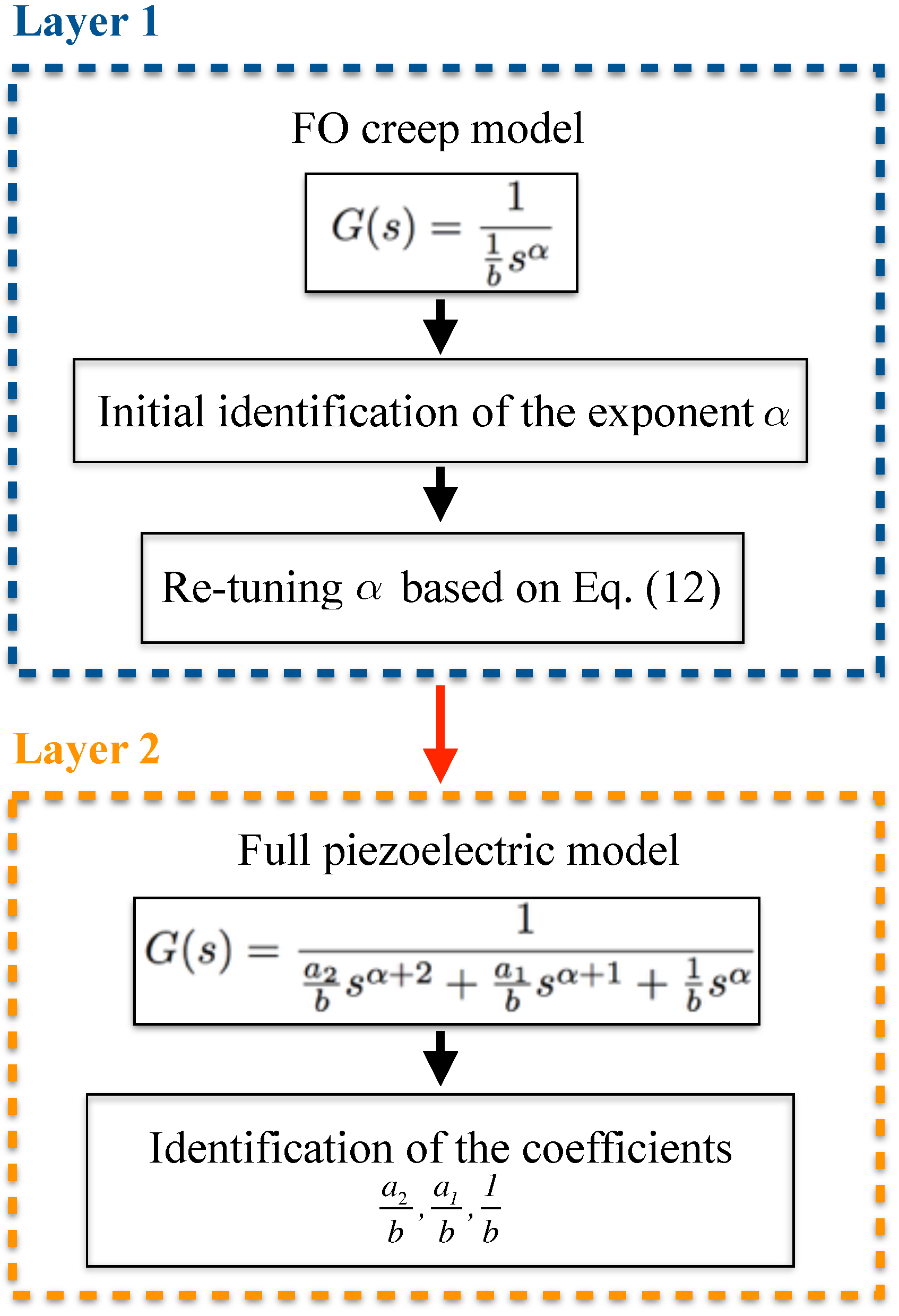
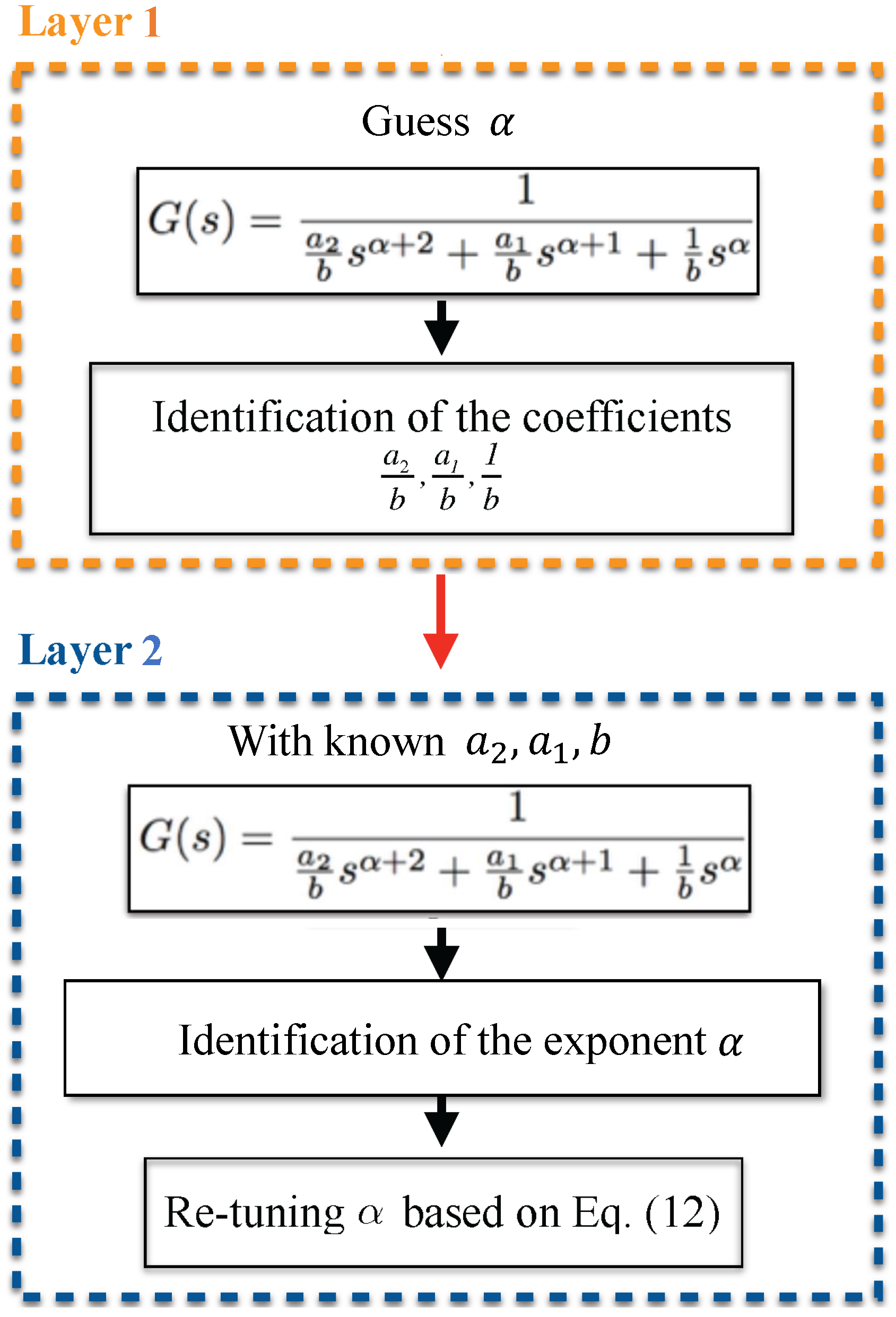
A two-layer trust region reflective algorithm is proposed for the parameter identification of the fractional-order piezoelectric model in Equation (4), which has four parameters to identify. This approach identifies the fractional-order exponent $\alpha$ in a separate layer than the integer-order polynomial coefficients $a_1,a_2$, and b. With this idea, the creep phenomenon and the mechanical resonant can be identified using different sampling times, time frames, and identification modes.

Remark 1.

It is observed that, when using the FOMCON package, the initial identified creep rate is not usually precise enough. This exponent is hence re-tuned based on the following strategy:

$$\alpha ={\alpha }_0\times {\displaystyle \frac{y_f^{*}-y_c^{*}}{{\widehat{y}}_f-{\widehat{y}}_c}},$$

(12)

where $y^{*}$ and $\widehat{y}$ are, respectively, the measured and estimated outputs with subscript f the final value and c corresponding to the time $t_c$, the time after which the mechanical response can be disregarded.

The strategy is hence as follows, as also shown schematically in Figure 1:

• Layer 1: The fractional-order exponent $\alpha$ is initially identified based on the creep model in Equation (5) with its numerator fixed as 1 and considering free identification mode. In this layer, a relatively greater sampling time can be used. Note that a value is also identified for ${\displaystyle \frac{1}{b}}$, which is disregarded as this parameter will be re-identified in the next layer. The estimated value for $\alpha$ is then re-tuned using Equation (12) to arrive at a more accurate creep rate.
• Layer 2: integer-order coefficients $a_1, a_2,$ and b are identified by using the determined $\alpha$ in layer 1. Here, the sampling time should be smaller while the time frame can be selected as $0<t<t_c$, with $t_c$ defined in Section 4. In this layer, the fix exponent mode is considered. Note that to alleviate the computational burden, the numerator can still be fixed at 1. As shown in Figure 1, with fixed exponents and numerator, the coefficients of the denominator ${\displaystyle \frac{a_2}{b}}, {\displaystyle \frac{a_1}{b}},$ and ${\displaystyle \frac{1}{b}}$ are identified. As the coefficient of $s^{\alpha }$ should be 1 (see Equation (4)), all three parameters $a_2,a_1$, and b are obtained.

Remark 2.

As stated above, one parameter is identified in layer 1, and three other parameters in layer 2. For online identification, one can first perform layer 2 in the time frame $0<t<t_c$ with a guess on α. Then, for $t>t_c$, α can be updated by performing layer 1. The initial guess on α does not need to be precisely accurate since the creep is mostly relevant when the input is constant or with a slow-changing rate, i.e., it is mostly the case in $t>t_c$ and not $0<t<t_c$.

As shown in Figure 2, for online identification, the idea of a two-layer trust region reflective algorithm can be performed as follows. First, the coefficients $a_2, a_1, b$ are identified by using an initial guess for $\alpha$ in $0<t<t_c$. Then, for $t>t_c$, using the identified coefficients from Layer 1, the creep rate $\alpha$ is found. In the end, this value can be retuned using Equation (12) for more accuracy.

Remark 3.

The readers interested in online identification of the FO creep model should note that GL approximation is recursive, i.e., the output of the fractional integrator is used to compute the new output. Therefore, one should be careful when the value of α changes as new samples arrive at the estimator. If, in that case, the computations need to be performed all over, this will require a batch implementation over a fixed time window. However, we believe that small changes in α may not interrupt the identification procedure, and it can proceed consecutively with the most recent estimated α.

5. Experimental Setups

Two experimental setups are utilized to validate the identification approach proposed in this paper, i.e.:

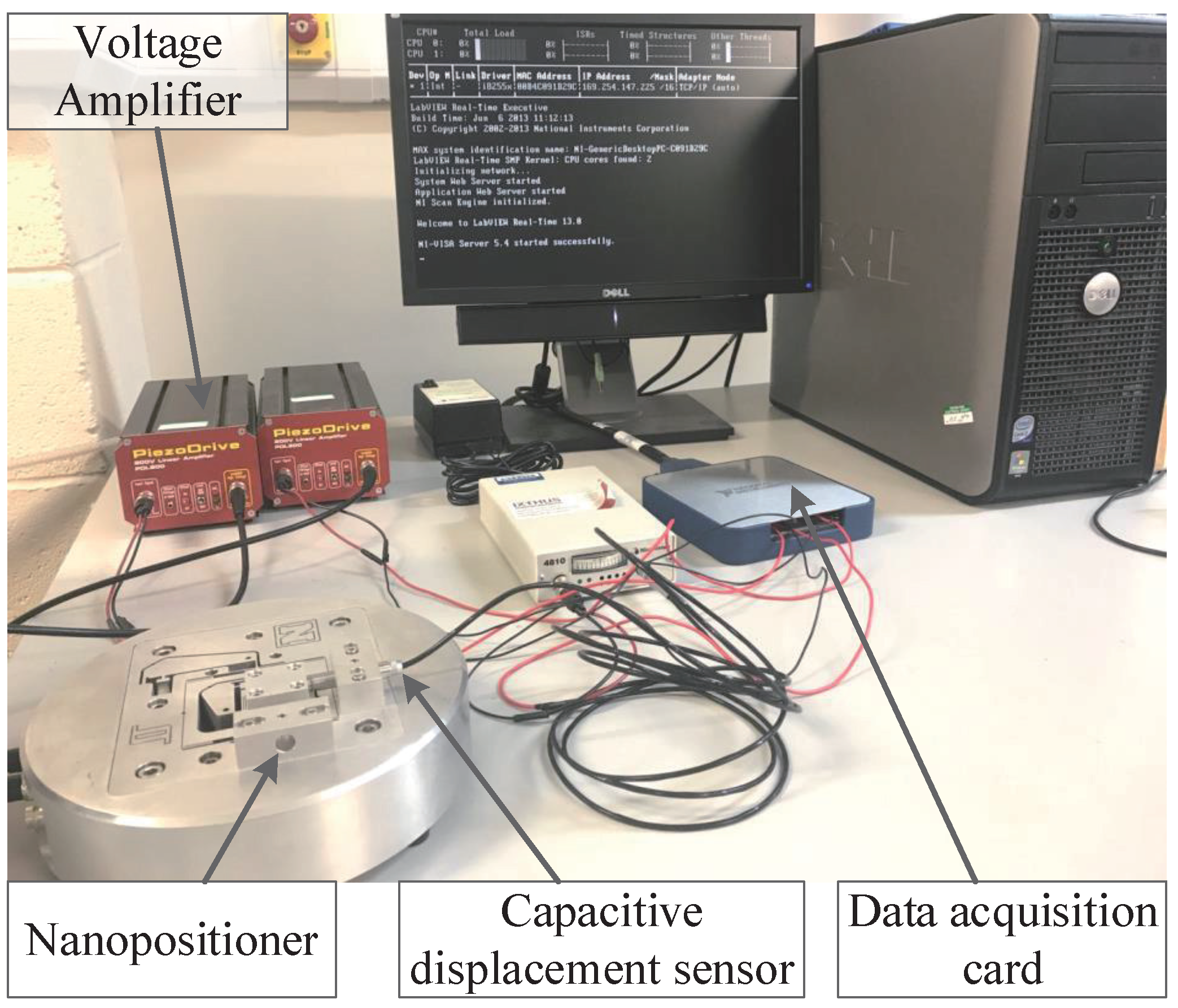
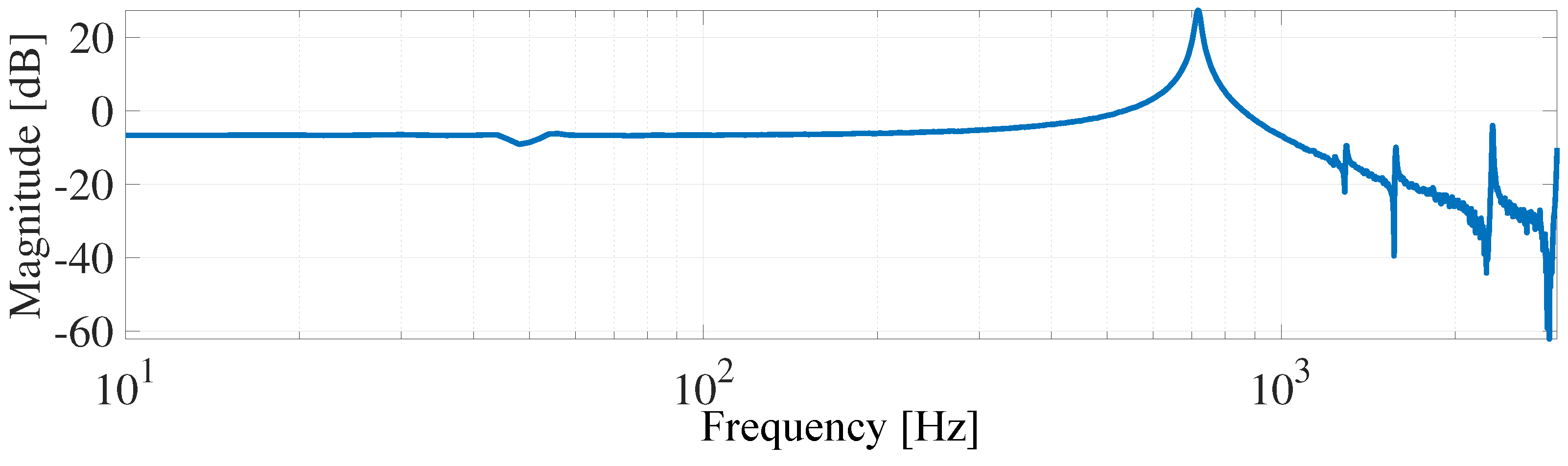
• Setup 1: A stack of piezo-actuated serial kinematic nanopositioning stage, designed by the EasyLab, University of Nevada, Reno, USA [62], is shown in Figure 3. A voltage amplifier supplies the actuation voltage in the range of 0–200 V, and the output displacement (±20 $\mathsf{\mu }$m) is measured by a high-resolution capacitive sensor in real-time [63]. Note that the experiment was conducted with an input of 0.7455 V, and the output was recorded every 0.005 s. As shown in Figure 4, the first resonant mode of the nanopositioner utilized in this paper is almost at 700 Hz. Therefore, the estimation time must be in the order of 1 ms, since, as stated in Section 4, the estimation time should be less than a period of the resonant mode frequency targeted, which provides the condition to tune the controller gains quickly enough. This figure also reveals some unmodeled dynamics that the identification approach needs to be robust against. As shown in Figure 4, there are several high-frequency resonant modes in the recorded frequency response, and the frequencies of the second and third modes are very close. Therefore, the third mode will influence the output signal and may lead to error in the system parameters identification as the system is modeled as a second-order resonant system.

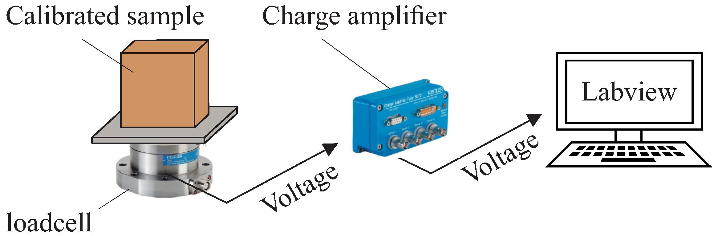
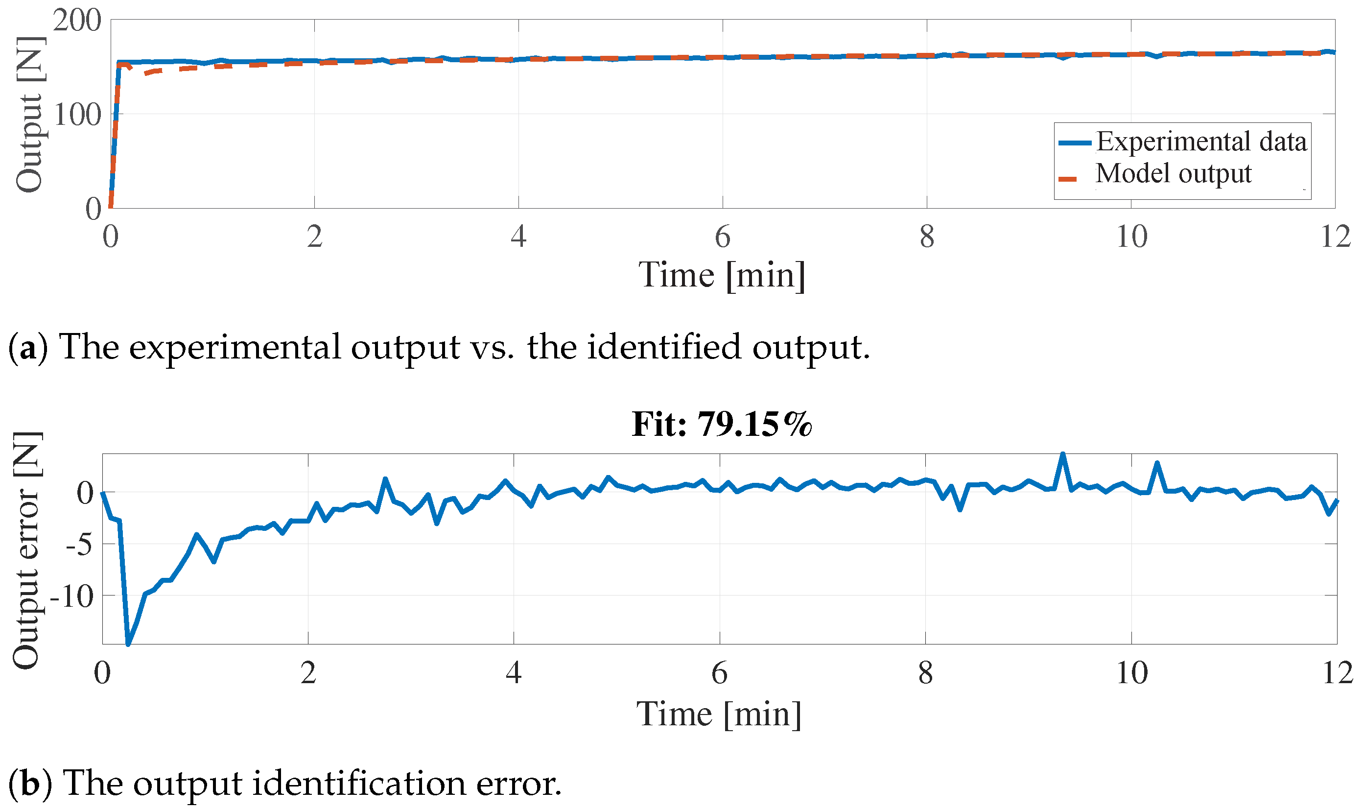
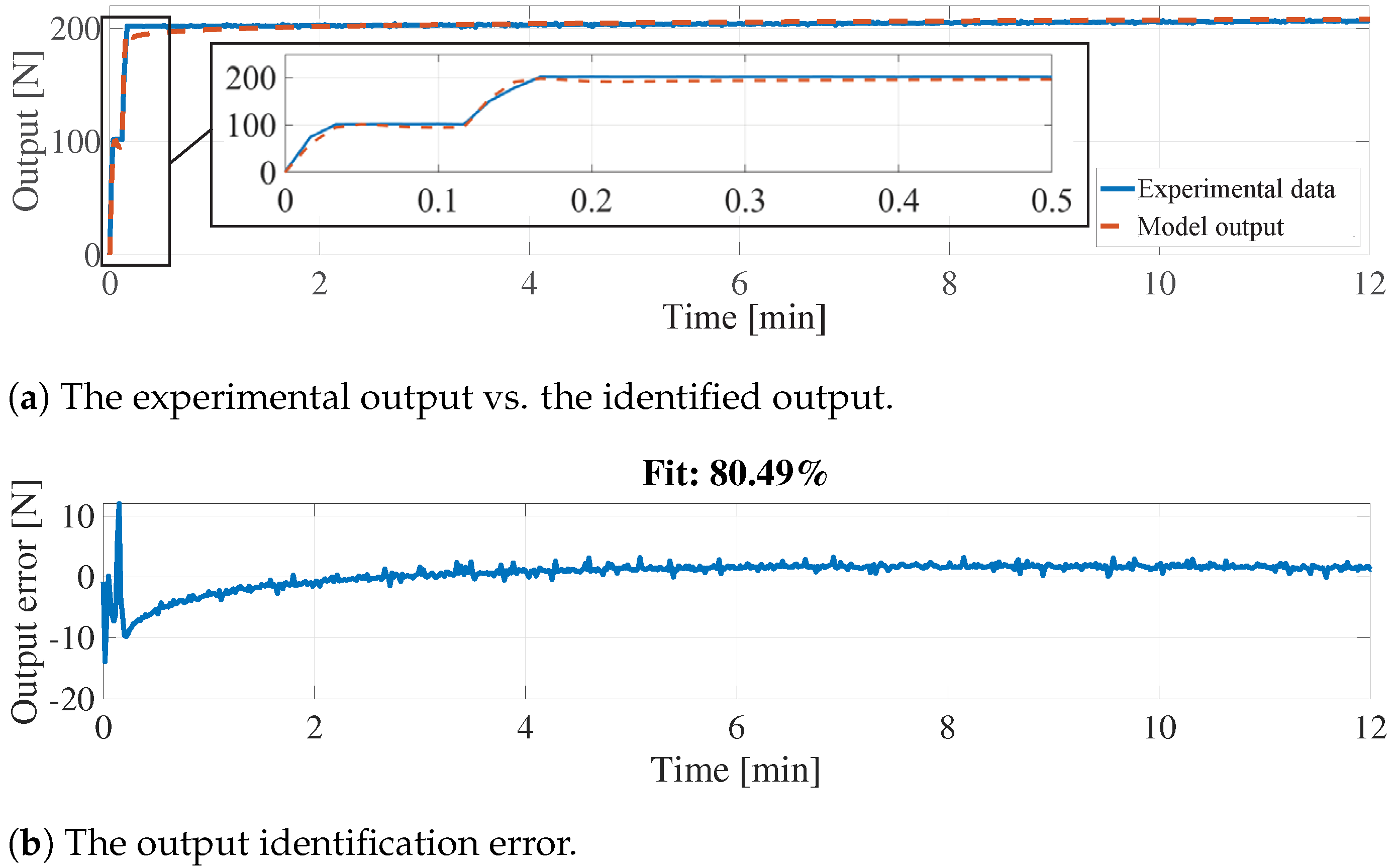
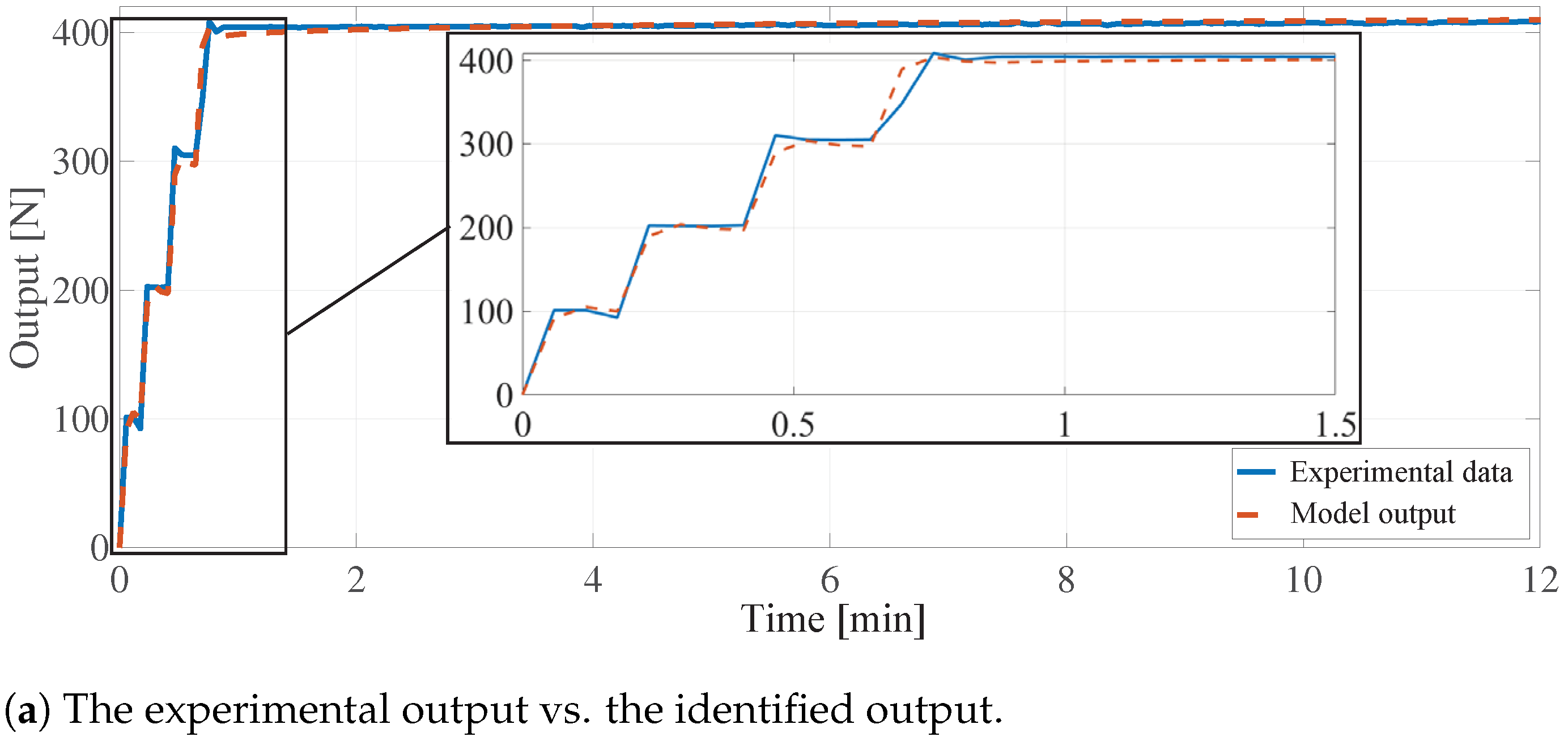
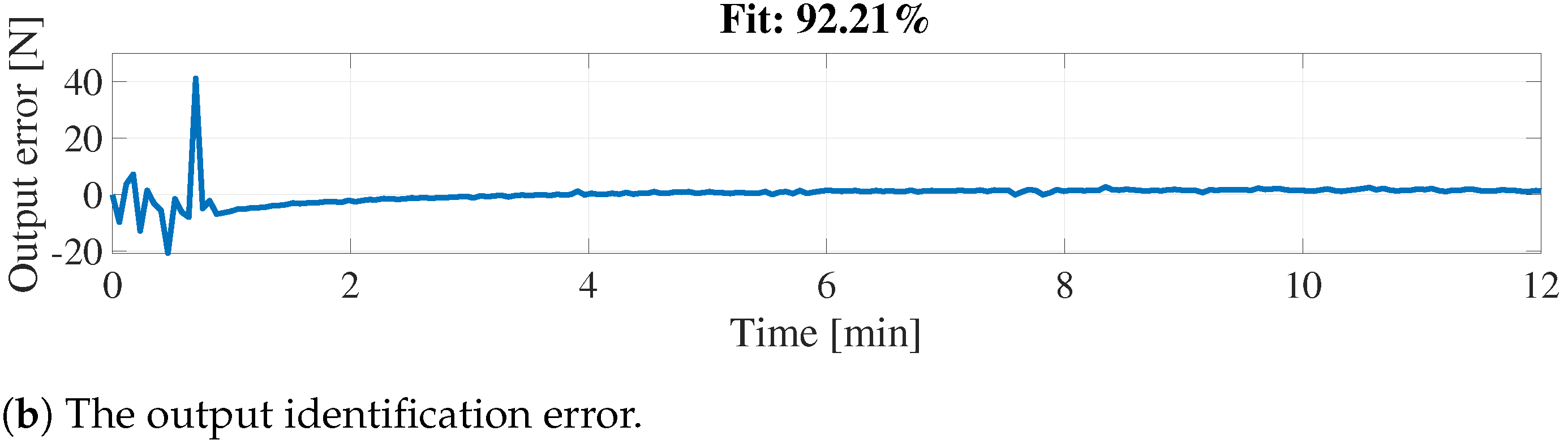
• Setup 2: Kistler 9272 four component dynamometer mounted on a vertical drill-string assembly, housed in the Drill-string Laboratory at the Centre for Applied Dynamics research (CADR), University of Aberdeen, Aberdeen, Scotland, UK [64]. A schematic of setup 2 is shown in Figure 5. This setup uses a stacked sensor configuration. The load-cell generates electric charge proportional to the measured forces and torques, relying on the principle of piezoelectricity. To convert the generated charges to corresponding voltage levels, a charge amplifier is required, for which a Kistler 5073A-type charge amplifier is utilized. Note that the experiment was conducted with different scenarios, i.e., one-step 50 N and 150 N loads, two-step 200 N input, and four-step 400 N input, and the output was recorded every 0.005 s.

6. Results and Discussion

In this section, the fractional-order piezoelectric model (Equation (4)) is identified based on the time-domain experimental step response, which demonstrates slow creep phenomenon. The validation of the two-layer trust region reflective algorithm, as proposed in Section 4, is shown by employing two experimental setups, presented in Section 5.

To obtain the time-domain response, the revised Grunwald–Letnikov method is utilized in this paper based on (3), as follows [17,39]:

$$y\left(t\right)={\displaystyle \frac{1}{{\sum }_{i=0}^2\frac{a_i}{h^{{\alpha }_i}}}}[u\left(t\right)-\sum _{i=0}^2(\frac{a_i}{h^{{\alpha }_i}}\sum _{j=1}^{\frac{t-t_0}{h}}{\omega }_j^{\left({\alpha }_i\right)}y(t-jh))],$$

(13)

with $a_0=1$, $a_1$ and $a_2$ as identified, ${\alpha }_0=\alpha , {\alpha }_1=\alpha +1,$ and ${\alpha }_2=\alpha +2$ with $\alpha$ identified. Note that the time step h should not be too large, as this may reduce the accuracy of the simulation. Conversely, it should not be too small, as this would result in unnecessarily long computation times. In Equation (13), ${\omega }_j^{\left(\alpha \right)}$ is recursively computed, as follows:

$${\omega }_j^{\left(\alpha \right)}=(1-{\displaystyle \frac{\alpha +1}{j}}){\omega }_{j-1}^{\left(\alpha \right)},j=1,2,\dots ,{\displaystyle \frac{t-t_0}{h}}$$

(14)

with ${\omega }_0^{\left(\alpha \right)}=1$.

As discussed earlier, the time-domain identification is considered a least squares problem that seeks the minimum of the error norm by searching for a set of parameters (Equation (8)) where the error is defined in Equation (10) as the difference between the identified and measured output. Note that since the natural frequency of the mechanical part is high, the output signal is prone to noise in the transient regime. However, generally speaking, the computation time of the identification increases dramatically when the experimental data have too many high-frequency contents. Therefore, the acquired output vector could be filtered using a low-pass filter that guarantees zero phase distortion. It is fortunate that this high-frequency dynamics can be disregarded in many applications [4]. Another idea that can alleviate the computational burden is that the time step can be considered bigger after the transient response, as the dynamics in this regime are slower, and hence not much information would be lost. Moreover, note that the output signal is shifted such that $y(t=0)$ is zero.

Applying the two-layer trust region reflective algorithm method, the governing piezoelectric model for setup 1 is identified as follows:

$$G\left(s\right)={\displaystyle \frac{0.1500}{s^{0.0133}(1-0.1200\times {10}^{-5}s+0.3298\times {10}^{-5}{s}^2)}}.$$

(15)

Figure 6 illustrates the experimental vs. the identified outputs, as well as the output identification error. As shown, the identified model fits 71.69 percent of the experimental data with almost 0.5 $\mu$m error norm, which demonstrates the efficacy of the proposed model. In this figure, two zoomed areas are demonstrated: one compares the experimental and identified outputs in the transient time, and the other illustrates the creep over time.

Remark 4.

The time required to run the code for the identification approach proposed in this paper depends on the size of the dataset utilized. In other words, the smaller the time step of the acquired data, the greater the convergence time, indicated by “Elapsed time” in the FOMCON toolbox. Specifically, for time steps of 0.005, 0.01, 0.02, and 0.03 s, the elapsed time of the creep model identification (Layer 1) is 29, 7, 2, and 1 s, respectively. For time steps greater than 0.04 s, the elapsed time is less than a second, which can be regarded as “fast identification”, with minimal loss of accuracy, as illustrated in Figure 7.

Figure 7 presents a zoomed-in view of the identified creep model output after performing Layer 1 with varying time steps for the input data. As shown, the plots for 0.005-s and 0.04-s time steps are relatively close. This indicates that for the identification of the creep rate in Layer 1, the proposed approach can be effectively utilized with larger time steps, meaning it does not necessarily require an extensive dataset.

Figure 8 shows a zoomed-in view of the identified full model output after performing both Layer 1 and Layer 2. Although the time step influences the accuracy of the identification in the transient regime, as stated before, the time frame in Layer 2 can be selected as $0<t<t_c$. Therefore, even with small time step, the size of the dataset utilized in Layer 2 is not large as the time frame is small.

The validation of the proposed two-layer trust region reflective identification is investigated by utilizing the experimental data of setup 2. With 50 N input force, the piezoelectric model is identified as follows:

$$G\left(s\right)={\displaystyle \frac{0.9922}{s^{0.085}(1-0.0363s+0.0013s^2)}},$$

(16)

which is compared with the experimental data in Figure 9. As illustrated, the identified output is 49.15 percent fit to the measured output.

Experimental setup 2 is again utilized to produce a new set of data with an input force of 150 N. In this case, the model is identified as follows:

$$G\left(s\right)={\displaystyle \frac{0.9792}{s^{0.037}(1-0.0172s+0.0006s^2)}},$$

(17)

which is 79.15 percent fit to the experimental data, as shown in Figure 10.

Remark 5.

In the full fractional-order piezoelectric model in Equation (4), α specifies the creep rate, b adjusts the error at the final time, and $a_2,a_1$ characterize the output in the transient condition, e.g., the overshoot and the settling time. Therefore, having reference data, for which the governing model is identified, can lead to intuitively approximating the parameters of an unknown model governing another set of data without running the identification procedure all over again. This is, of course, applicable when high modeling accuracy is not essential.

Figure 11 and Figure 12 illustrate the identified piezoelectric model for a two-step and four-step input. Note that to obtain these figures the identification algorithm is performed only once. The resulting identified transfer functions are as follows:

$$G\left(s\right)={\displaystyle \frac{0.9861}{s^{0.0173}(1+0.0032s+0.8805\times {10}^{-4}{s}^2)}},$$

(18)

for the two-step input scenario, and

$$G\left(s\right)={\displaystyle \frac{0.9954}{s^{0.0094}(1-0.0017s+0.2991\times {10}^{-3}{s}^2)}},$$

(19)

for the four-step scenario. These figures show the validity of the proposed identification approach for other input functions than a simple step.

In brief, the results of two experimental set-ups validate the efficacy of the fractional-order modeling and the proposed two-layer identification for piezoelectric actuators/sensors model with consideration of the creep phenomenon.

7. Conclusions

Precise modeling and identification are increasingly demanded for micro/nano-scale positioning in low frequencies, which performance is deteriorated due to the creep phenomenon. To improve modeling precision, fractional-order models have been presented in recent years. In this paper, a piezoelectric fractional-order model is employed according to the properties of the creep effect. A parameter identification approach, named the two-layer trust region reflective method, is proposed, aiming at a faster identification. In this method, the fractional-order exponent, describing the creep phenomenon, is identified in a separate layer as the integer-order coefficients, describing the mechanical resonant, with different time frames and sampling times. This idea is hence appropriate for applications that need online identification and control.

The effectiveness and validation of the proposed identification technique are experimentally shown by using the data acquired from two different experimental setups. The first setup is a piezo-actuated serial kinematic nanopositioner, and the second setup is a dynamometer, relying on the principle of piezoelectricity, mounted on a vertical drill-string assembly. Step responses of both setups show slow creep phenomenon. The time-domain identification is then performed, seeking a set of parameters that minimizes the difference between the identified and measured output. The measured output vector is first filtered using a low-pass filter that guarantees zero phase distortion since the signal is prone to noise in the transient regime due to the high natural frequency of the mechanical part. To obtain the time-domain response of the identified model, the revised Grunwald–Letnikov method is utilized. The validity of the proposed identification approach is also demonstrated for other input functions than a simple step, i.e., two-step and four-step scenarios.

The proposed fractional-order identification of the creep phenomenon is a stepping stone toward improved control schemes, aiming at positioning precision, which is under investigation by the authors in their future work.

References

1. Sabarianand, D.; Karthikeyan, P.; Muthuramalingam, T. A review on control strategies for compensation of hysteresis and creep on piezoelectric actuators based micro systems. Mech. Syst. Signal Process. 2020, 140, 106634. [Google Scholar] [CrossRef]
2. Yang, C.; Youcef-Toumi, K. Principle, implementation, and applications of charge control for piezo-actuated nanopositioners: A comprehensive review. Mech. Syst. Signal Process. 2022, 171, 108885. [Google Scholar] [CrossRef]
3. Chen, J.; Gong, L.; Meng, R. Application of Fractional Calculus in Predicting the Temperature-Dependent Creep Behavior of Concrete. Fractal Fract. 2024, 8, 482. [Google Scholar] [CrossRef]
4. Liu, Y.; Shan, J.; Qi, N. Creep modeling and identification for piezoelectric actuators based on fractional-order system. Mechatronics 2013, 23, 840–847. [Google Scholar] [CrossRef]
5. El-Rifai, O.M.; Youcef-Toumi, K. Creep in piezoelectric scanners of atomic force microscopes. In Proceedings of the 2002 American Control Conference (IEEE Cat. No. CH37301), IEEE, Anchorage, AK, USA, 8–10 May 2002; Volume 5, pp. 3777–3782. [Google Scholar]
6. Ge, R.; Wang, X.; Long, J.; Chen, Z.; Zhang, X. Creep modeling and control methods of piezoelectric actuators based on fractional order theory. In Proceedings of the Sixth International Conference on Electromechanical Control Technology and Transportation (ICECTT 2021), Chongqing, China, 14–16 May 2021; SPIE: San Francisco, CA, USA, 2022; Volume 12081, pp. 71–80. [Google Scholar]
7. Voda, A.; Charef, A.; Idiou, D.; Machado, M.M.P. Creep modeling for piezoelectric actuators using fractional order system of commensurate order. In Proceedings of the 2017 21st International Conference on System Theory, Control and Computing (ICSTCC), IEEE, Sinaia, Romania, 19–21 October 2017; pp. 120–125. [Google Scholar]
8. Tominaga, K.; Hamai, K.; Gupta, B.; Kudoh, Y.; Takashima, W.; Prakash, R.; Kaneto, K. Suppression of electrochemical creep by cross-link in polypyrrole soft actuators. Phys. Procedia 2011, 14, 143–146. [Google Scholar] [CrossRef]
9. Gu, G.Y.; Gupta, U.; Zhu, J.; Zhu, L.M.; Zhu, X. Modeling of viscoelastic electromechanical behavior in a soft dielectric elastomer actuator. IEEE Trans. Robot. 2017, 33, 1263–1271. [Google Scholar] [CrossRef]
10. Pesotski, D.; Janocha, H.; Kuhnen, K. Adaptive compensation of hysteretic and creep non-linearities in solid-state actuators. J. Intell. Mater. Syst. Struct. 2010, 21, 1437–1446. [Google Scholar] [CrossRef]
11. Yang, Q.; Jagannathan, S. Creep and hysteresis compensation for nanomanipulation using atomic force microscope. Asian J. Control 2009, 11, 182–187. [Google Scholar] [CrossRef]
12. Panja, P. Dynamics of a fractional order predator-prey model with intraguild predation. Int. J. Model. Simul. 2019, 39, 256–268. [Google Scholar] [CrossRef]
13. Deressa, C.T.; Duressa, G.F. Investigation of the dynamics of COVID-19 with SEIHR nonsingular and nonlocal kernel fractional model. Int. J. Model. Simul. 2022, 42, 1030–1048. [Google Scholar] [CrossRef]
14. Qureshi, S.; Abro, K.A.; Gómez-Aguilar, J. On the numerical study of fractional and non-fractional model of nonlinear Duffing oscillator: A comparison of integer and non-integer order approaches. Int. J. Model. Simul. 2022, 43, 362–375. [Google Scholar] [CrossRef]
15. Xu, Y.; Luo, Y.; Luo, X.; Chen, Y.; Liu, W. Fractional-Order Modeling of Piezoelectric Actuators with Coupled Hysteresis and Creep Effects. Fractal Fract. 2023, 8, 3. [Google Scholar] [CrossRef]
16. Li, J.; Hu, B.; Sheng, J.; Huang, L. A Fractional-Order Creep-Damage Model for Carbonaceous Shale Describing Coupled Damage Caused by Rainfall and Blasting. Fractal Fract. 2024, 8, 459. [Google Scholar] [CrossRef]
17. Chen, Y.; Petras, I.; Xue, D. Fractional order control-a tutorial. In Proceedings of the 2009 American Control Conference, IEEE, St. Louis, MO, USA, 10–12 June 2009; pp. 1397–1411. [Google Scholar]
18. Shahri, E.S.A.; Alfi, A.; Tenreiro Machado, J. Stabilization of fractional-order systems subject to saturation element using fractional dynamic output feedback sliding mode control. J. Comput. Nonlinear Dyn. 2017, 12, 031014. [Google Scholar] [CrossRef]
19. Delavari, H.; Heydarinejad, H. Fractional-order backstepping sliding-mode control based on fractional-order nonlinear disturbance observer. J. Comput. Nonlinear Dyn. 2018, 13, 111009. [Google Scholar] [CrossRef]
20. Muñoz-Vázquez, A.J.; Parra-Vega, V.; Sánchez-Orta, A. Fractional-Order Nonlinear Disturbance Observer Based Control of Fractional-Order Systems. J. Comput. Nonlinear Dyn. 2018, 13, 071007. [Google Scholar] [CrossRef]
21. Muñoz-Vázquez, A.J.; Martínez-Reyes, F. Output feedback fractional integral sliding mode control of robotic manipulators. J. Comput. Nonlinear Dyn. 2019, 14, 054502. [Google Scholar] [CrossRef]
22. Soukkou, A.; Soukkou, Y.; Haddad, S.; Benghanem, M.; Rabhi, A. Finite-Time Synchronization of Fractional-Order Energy Resources Demand-Supply Hyperchaotic Systems Via Fractional-Order Prediction-Based Feedback Control Strategy with Bio-Inspired Multiobjective Optimization. J. Comput. Nonlinear Dyn. 2023, 18, 031003. [Google Scholar] [CrossRef]
23. Muñoz-Vázquez, A.J.; Treesatayapun, C. Discrete-Time Adaptive Fractional Nonlinear Control Using Fuzzy Rules Emulating Networks. J. Comput. Nonlinear Dyn. 2023, 18, 071002. [Google Scholar] [CrossRef]
24. San-Millan, A.; Feliu-Batlle, V.; Aphale, S.S. Fractional order implementation of Integral Resonant Control–A nanopositioning application. ISA Trans. 2018, 82, 223–231. [Google Scholar] [CrossRef]
25. Conejero, J.A.; Franceschi, J.; Picó-Marco, E. Fractional vs. ordinary control systems: What does the fractional derivative provide? Mathematics 2022, 10, 2719. [Google Scholar] [CrossRef]
26. Liu, Y.; Shan, J.; Gabbert, U.; Qi, N. Hysteresis and creep modeling and compensation for a piezoelectric actuator using a fractional-order Maxwell resistive capacitor approach. Smart Mater. Struct. 2013, 22, 115020. [Google Scholar] [CrossRef]
27. Liu, L.; Yun, H.; Li, Q.; Ma, X.; Chen, S.L.; Shen, J. Fractional order based modeling and identification of coupled creep and hysteresis effects in piezoelectric actuators. IEEE/ASME Trans. Mechatron. 2020, 25, 1036–1044. [Google Scholar] [CrossRef]
28. Tashakori, S.; Vaziri, V.; Aphale, S.S. A comparative quantification of existing creep models for piezoactuators. In Proceedings of the 10th International Conference on Wave Mechanics and Vibrations, WMVC2022, Lisbon, Portugal, 4–6 July 2022; Springer: Cham, Switzerland, 2022. [Google Scholar]
29. Le Lay, L. Identification Fréquentielle et Temporelle par Modèle non Entier. Ph.D. Thesis, University of Bordeaux, Bordeaux, France, 1998. Available online: http://www.theses.fr/1998BOR10605 (accessed on 27 October 2024).
30. Malti, R.; Aoun, M.; Sabatier, J.; Oustaloup, A. Tutorial on system identification using fractional differentiation models. IFAC Proc. Vol. 2006, 39, 606–611. [Google Scholar] [CrossRef]
31. Malti, R.; Victor, S.p.; Nicolas, O.; Oustaloup, A. System identification using fractional models: State of the art. In Proceedings of the International Design Engineering Technical Conferences and Computers and Information in Engineering Conference, Las Vegas, NV, USA, 4–7 September 2007; Volume 4806, pp. 295–304. [Google Scholar]
32. Malti, R.; Victor, S.; Oustaloup, A. Advances in system identification using fractional models. J. Comput. Nonlinear Dyn. 2008, 3. [Google Scholar] [CrossRef]
33. Gupta, R.; Gairola, S.; Diwiedi, S. Fractional order system identification and controller design using PSO. In Proceedings of the 2014 Innovative Applications of Computational Intelligence on Power, Energy and Controls with their impact on Humanity (CIPECH) IEEE, Ghaziabad, India, 28–29 November 2014; pp. 149–153. [Google Scholar]
34. Liu, L.; Shan, L.; Jiang, C.; Dai, Y.; Liu, C.; Qi, Z. Parameter identification of the fractional-order systems based on a modified PSO algorithm. J. Southeast Univ. (Engl. Ed.) 2018, 34, 6–14. [Google Scholar]
35. Zhou, S.; Cao, J.; Chen, Y. Genetic algorithm-based identification of fractional-order systems. Entropy 2013, 15, 1624–1642. [Google Scholar] [CrossRef]
36. Zhang, L.; Chen, Y.; Sun, R.; Jing, S.; Yang, B. A task scheduling algorithm based on PSO for grid computing. Int. J. Comput. Intell. Res. 2008, 4, 37–43. [Google Scholar] [CrossRef]
37. Oustaloup, A.; Melchior, P.; Lanusse, P.; Cois, O.; Dancla, F. The CRONE toolbox for Matlab. In Proceedings of the CACSD, Conference Proceedings-IEEE International Symposium on Computer-Aided Control System Design (Cat. No. 00TH8537) IEEE, Anchorage, AK, USA, 25–27 September 2000; pp. 190–195. [Google Scholar]
38. Valerio, D.; Da Costa, J.S. Ninteger: A non-integer control toolbox for MatLab. In Proceedings of the Fractional Differentiation and Its Applications; ENSEIRB: Bordeaux, France, 2004. [Google Scholar]
39. Tepljakov, A.; Petlenkov, E.; Belikov, J. FOMCON: A MATLAB toolbox for fractional-order system identification and control. Int. J. Microelectron. Comput. Sci. 2011, 2, 51–62. [Google Scholar]
40. Xue, D.; Chen, Y.; Atherton, D.P. Linear Feedback Control: Analysis and Design with MATLAB; SIAM: Philadelphia, PA, USA, 2007. [Google Scholar]
41. Jumarie, G. Modified Riemann–Liouville derivative and fractional Taylor series of nondifferentiable functions further results. Comput. Math. Appl. 2006, 51, 1367–1376. [Google Scholar] [CrossRef]
42. Atangana, A.; Gómez-Aguilar, J. Numerical approximation of Riemann–Liouville definition of fractional derivative: From Riemann–Liouville to Atangana-Baleanu. Numer. Methods Partial. Differ. Equ. 2018, 34, 1502–1523. [Google Scholar] [CrossRef]
43. Scherer, R.; Kalla, S.L.; Tang, Y.; Huang, J. The Grünwald–Letnikov method for fractional differential equations. Comput. Math. Appl. 2011, 62, 902–917. [Google Scholar] [CrossRef]
44. Ortigueira, M.D.; Machado, J.T. What is a fractional derivative? J. Comput. Phys. 2015, 293, 4–13. [Google Scholar] [CrossRef]
45. Tepljakov, A. FOMCON: Fractional-order modeling and control toolbox. In Fractional-Order Modeling and Control of Dynamic Systems; Springer: Cham, Switzerland, 2017; pp. 107–129. [Google Scholar]
46. Sabatier, J.; Farges, C. Initial value problems should not be associated with fractional model descriptions whatever the derivative definition used. AIMS Math 2021, 6, 11318–11329. [Google Scholar] [CrossRef]
47. Kilbas, A.A.; Srivastava, H.M.; Trujillo, J.J. Theory and Applications of Fractional Differential Equations; Springer: Cham, Switzerland, 2006; Volume 204. [Google Scholar]
48. Monje, C.A.; Chen, Y.; Vinagre, B.M.; Xue, D.; Feliu-Batlle, V. Fractional-Order Systems and Controls: Fundamentals and Applications; Springer Science & Business Media: Cham, Switzerland, 2010. [Google Scholar]
49. Yuan, Z.; Zhou, S.; Zhang, Z.; Xiao, Z.; Hong, C.; Chen, X.; Zeng, L.; Li, X. Piezo-actuated smart mechatronic systems: Nonlinear modeling, identification, and control. Mech. Syst. Signal Process. 2024, 221, 111715. [Google Scholar] [CrossRef]
50. Salapaka, S.; Sebastian, A.; Cleveland, J.P.; Salapaka, M.V. High bandwidth nano-positioner: A robust control approach. Rev. Sci. Instrum. 2002, 73, 3232–3241. [Google Scholar] [CrossRef]
51. Mohammadzaheri, M.; Grainger, S.; Bazghaleh, M. A system identification approach to the characterization and control of a piezoelectric tube actuator. Smart Mater. Struct. 2013, 22, 105022. [Google Scholar] [CrossRef]
52. Moore, S.I.; Yong, Y.K.; Omidbeike, M.; Fleming, A.J. Serial-kinematic monolithic nanopositioner with in-plane bender actuators. Mechatronics 2021, 75, 102541. [Google Scholar] [CrossRef]
53. Aphale, S.; Fleming, A.J.; Moheimani, S. High speed nano-scale positioning using a piezoelectric tube actuator with active shunt control. Micro Nano Lett. 2007, 2, 9–12. [Google Scholar] [CrossRef]
54. Kuiper, S.; Schitter, G. Active damping of a piezoelectric tube scanner using self-sensing piezo actuation. Mechatronics 2010, 20, 656–665. [Google Scholar] [CrossRef]
55. Fleming, A.J.; Moheimani, S.R. Sensorless vibration suppression and scan compensation for piezoelectric tube nanopositioners. IEEE Trans. Control Syst. Technol. 2005, 14, 33–44. [Google Scholar] [CrossRef]
56. Das, S. Functional Fractional Calculus; Springer: Berlin/Heidelberg, Germany, 2011; Volume 1. [Google Scholar]
57. Chen, Y.; Petras, I.; Vinagre, B. A List of Laplace and Inverse Laplace Transforms Related to Fractional Order Calculus. 2001. Available online: http://people.tuke.sk/ivo.petras/foclaplace.pdf (accessed on 30 November 2001).
58. Bellavia, S.; Gratton, S.; Riccietti, E. A Levenberg–Marquardt method for large nonlinear least-squares problems with dynamic accuracy in functions and gradients. Numer. Math. 2018, 140, 791–825. [Google Scholar] [CrossRef]
59. Gavin, H.P. The Levenberg–Marquardt Algorithm for Nonlinear Least Squares Curve-Fitting Problems; Department of Civil and Environmental Engineering, Duke University: Durham, NC, USA, 2019; Volume 19. [Google Scholar]
60. Le, T.M.; Fatahi, B.; Khabbaz, H.; Sun, W. Numerical optimization applying trust-region reflective least squares algorithm with constraints to optimize the non-linear creep parameters of soft soil. Appl. Math. Model. 2017, 41, 236–256. [Google Scholar] [CrossRef]
61. Ahsan, M.; Choudhry, M.A. System identification of an airship using trust region reflective least squares algorithm. Int. J. Control Autom. Syst. 2017, 15, 1384–1393. [Google Scholar] [CrossRef]
62. Fairbairn, M.W.; Moheimani, S.R. Control techniques for increasing the scan speed and minimizing image artifacts in tapping-mode atomic force microscopy: Toward video-rate nanoscale imaging. IEEE Control Syst. Mag. 2013, 33, 46–67. [Google Scholar]
63. Babarinde, A.K.; Li, L.; Zhu, L.; Aphale, S.S. Experimental validation of the simultaneous damping and tracking controller design strategy for high-bandwidth nanopositioning—A PAVPF approach. IET Control Theory Appl. 2020, 14, 3506–3514. [Google Scholar] [CrossRef]
64. Vaziri, V.; Oladunjoye, I.O.; Kapitaniak, M.; Aphale, S.S.; Wiercigroch, M. Parametric analysis of a sliding-mode controller to suppress drill-string stick-slip vibration. Meccanica 2020, 55, 2475–2492. [Google Scholar] [CrossRef]
Figure 1. The general idea of the two-layer trust region reflective identification algorithm for the fractional-order piezoelectric model.
Actuators 13 00534 g001
Figure 2. Two-layer trust region reflective algorithm for online identification of the fractional-order piezoelectric model.
Actuators 13 00534 g002
Figure 3. Experimental setup 1: two-axis piezo-actuated serial kinematic nanopositioning stage [63].
Actuators 13 00534 g003
Figure 4. Frequency response function of the x−axis and y−axis in the experimental setup 1.
Actuators 13 00534 g004
Figure 5. Experimental setup 1, including Kistler 9272 load-cell, a four component dynamometer, and ICAM5073A charge amplifier.
Actuators 13 00534 g005
Figure 6. Identification of the piezoelectric model for setup 1.
Actuators 13 00534 g006
Figure 7. Comparison of the identified creep model outputs (Layer 1) using different time steps for the input data.
Actuators 13 00534 g007
Figure 8. Comparison of the identified full model outputs (Layers 1 and 2) using different time steps for the input data.
Actuators 13 00534 g008
Figure 9. Identification of the piezoelectric model for setup 2 with 50 N input.
Actuators 13 00534 g009
Figure 10. Identification of the piezoelectric model for setup 2 with 150 N input.
Actuators 13 00534 g010
Figure 11. Identification of the piezoelectric model for setup 2 with a two-step input.
Actuators 13 00534 g011
Figure 12. Identification of the piezoelectric model for setup 2 with a four-step input.
Actuators 13 00534 g012aActuators 13 00534 g012b
Disclaimer/Publisher’s Note: The statements, opinions and data contained in all publications are solely those of the individual author(s) and contributor(s) and not of MDPI and/or the editor(s). MDPI and/or the editor(s) disclaim responsibility for any injury to people or property resulting from any ideas, methods, instructions or products referred to in the content.