Abstract
The compressibility of air, the uncertainty of dynamic models, and the existence of friction make pneumatic servo systems exhibit strong nonlinearity. Furthermore, the confluence of pneumatic-system nonlinearity and interference from the position system induces oscillations within the system, thereby posing a formidable challenge for achieving precise torque control. This study ensures precise torque control in a pneumatic actuator amid interference from the position system and proposes a novel active disturbance-rejection controller integrated with a Kalman filter. Firstly, in response to the oscillation stemming from the inherent nonlinearity of the pneumatic system and interference from the position system, this paper designs an active disturbance-rejection controller (ADRC) with robust anti-interference capabilities aimed at mitigating system oscillations. Secondly, to address the issue of sensor noise interfering with the ADRC and causing system oscillation, a first-order Kalman filter is designed to provide real-time and more accurate state estimation, effectively reducing oscillations and improving the robustness of the system. Finally, using the Lyapunov stability theory, the effectiveness of both the nonlinear extended observer and the convergence of the nonlinear error-state controller in the ADRC is proven. Experimental results indicate that the proposed controller reduces system oscillations and improves control accuracy.
1. Introduction
Pneumatic rotary actuators are extensively employed in robotics, medicine, polishing, and other relevant fields [1,2,3] owing to their advantages, such as low cost, cleanliness, and uncomplicated design [4,5]. The precise control of torque in pneumatic rotary actuators is a vital concern in pneumatic servo systems [6]. However, the presence of external disturbance, the compressibility of air, the uncertain dynamic model, and friction render the pneumatic servo system a highly nonlinear system [7,8]. The external disturbance and the nonlinearity in the pneumatic system pose significant challenges to achieving accurate control of torque. Researchers have implemented various control strategies to enhance the control performance of pneumatic-torque servo systems. Sliding-mode controllers are employed for precise force control of the cylinders, using cost functions to counteract the nonlinearity of the systems and disturbances from uncertain models [9,10]. However, they require relatively accurate models and are prone to oscillations on the sliding-mode surfaces. Moreover, backstepping control technology is utilized for controller design and analysis, compensating for the nonlinearity, uncertainty, and external disturbances of the pneumatic system by estimating the inverse model of the system to achieve improved control performance [11,12]. However, it demands a high level of model accuracy. Additionally, adaptive control strategies are applied to force control in pneumatic servo systems, achieving parameter adaptation to address model uncertainty and friction issues [13,14]. However, these strategies require precise models, and measurement errors and sensor noise can lead to parameter estimation errors. Most of the above methods are based on accurate models, but due to the time-varying characteristics of pneumatic servo systems, obtaining precise models is challenging.
Therefore, some scholars have adopted non-model-based digital control strategies. The improved fuzzy PID controller is applied to constant-force polishing, utilizing a fuzzy-logic strategy to approximate the nonlinearity of the pneumatic system. Moreover, the fuzzy PID strategy, not which does not rely on a model, addresses the issue of model uncertainty [15,16]. An intelligent PID controller, generated through the combination of the Fictitious Reference Iterative Tuning method and the Model-Free Adaptive Control method, avoids the difficulty of obtaining precise models through a data-driven approach [17]. However, the improved PID control strategy mentioned above still requires enhancement in terms of robustness. A novel non-model-based adaptive control, employing a data-driven approach, eliminates the need for process modeling [18]. However, its robustness in the presence of strong external disturbances requires improvement. The aforementioned data-driven control strategy addresses the challenge of obtaining models, but its robustness needs improvement when facing strong external disturbances. Therefore, to address disturbances from external position systems and friction, the system also needs to have strong robustness. This paper proposes an active disturbance-rejection controller integrated with a Kalman filter (ADRCKF) that is not model-based and has strong anti-interference capability.
As a typical data-driven controller, the active disturbance-rejection control technique has become increasingly popular in various fields, such as in satellite cameras [19] and amphibious multi-rotor drones [20], owing to its reduced dependence on precise models and strong disturbance-rejection capability [21]. In practical engineering applications, obtaining precise models is not always feasible. The effectiveness of the active disturbance-rejection controller (ADRC), which does not rely on precise models and boasts robust anti-disturbance capabilities, is credited to the use of an extended observer. The extended-state observer (ESO) is not dependent on a specified model of the observed object and can estimate and compensate for the inner nonlinear part of the system and external disturbance in real time [22]. Extended-state observers can be categorized as linear extended observers and nonlinear extended observers. The linear extended observer is relatively simpler to design, and its parameters are more convenient to adjust compared with a nonlinear extended observer. However, a nonlinear extended-state observer offers better performance for complex nonlinear systems [23]. Thus, this paper proposes a nonlinear ESO for real-time observation of friction in the pneumatic rotary actuator as well as of disturbances from air compressibility and the position system in a complex pneumatic system. It expands these disturbances into a total disturbance for compensation. Although the ADRC demonstrates effective performance in dealing with the complex nonlinearity and external disturbances in pneumatic systems, it also has certain limitations. The ADRC demands a high level of purity in the feedback signal, and the presence of noise can impact its control performance, leading to system oscillations [24]. Therefore, this paper designs a Kalman filter for real-time state estimation to enhance the purity of the feedback signal and improve the performance of the ADRC. The Kalman filter is a recursive filter that continuously updates estimates in real time amidst measurement errors and system noise [25]. Integrating a Kalman filter into an ADRC enables accurate state estimation in the presence of system noise and measurement errors, thereby improving control accuracy and stability. Studying the theory and practice of this field holds great significance as it serves as a source of inspiration for further research work.
This paper presents improvements to the active disturbance-rejection controller by introducing an integrated Kalman-filter-based active disturbance-rejection controller. The objective is to suppress system oscillations in the presence of external position disturbances, ensuring precise control of the aerodynamic torque system. Due to the interference of the position system with the torque system, oscillations occur in the torque system. The torque sensor is connected to both the torque and position systems, and when the torque system oscillates, the torque sensor vibrates as well. Mechanical vibrations can introduce noise into the torque sensor, and the active disturbance-rejection controller is susceptible to the influence of sensor noise, leading to the drawback of oscillations [23].
This paper integrates a Kalman filter into the active disturbance-rejection controller for real-time filtering and state estimation, effectively mitigating system oscillations and improving system accuracy. In comparison with the standard active disturbance-rejection controller, the integrated Kalman-filter-based active disturbance-rejection controller demonstrates a 34% improvement in control accuracy during a sinusoidal-torque tracking experiment with a frequency of 0.5 Hz.
The main contributions of this article are summarized as follows:
- (1)
- An active disturbance-rejection torque controller integrated with a Kalman filter is presented.
- (2)
- The control accuracy of the pneumatic servo system can be greatly enhanced by the NLESO, which estimates and compensates for external disturbances and nonlinearity.
- (3)
- The Kalman filter is designed to perform real-time filtering, effectively addressing sensor-generated noise and reducing system oscillations; thus, the control precise of the system is advanced.
2. Materials and Methods
2.1. System Structure
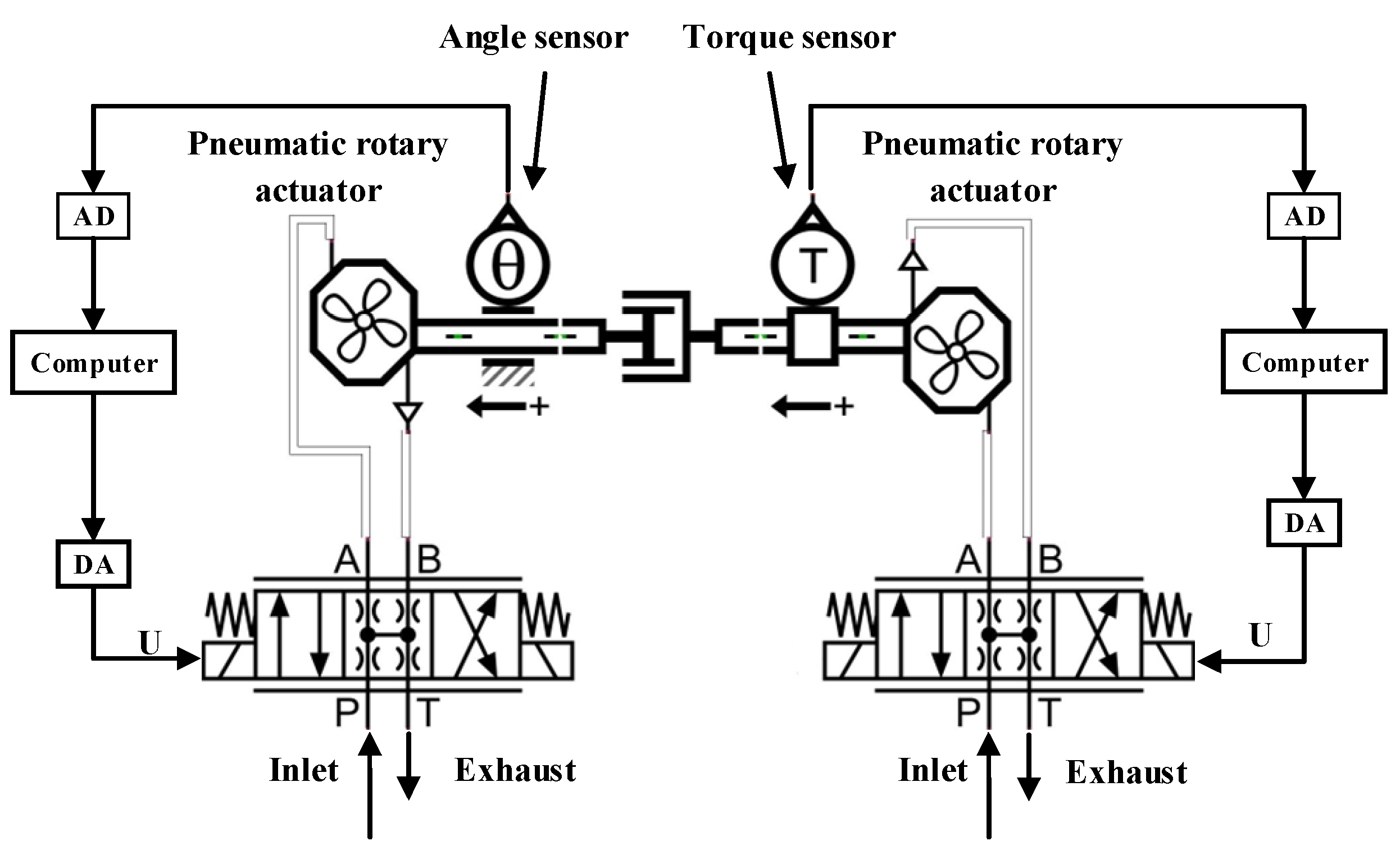
The control diagram of the pneumatic-torque servo system based on positional interference is illustrated in Figure 1.
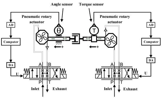
Figure 1.
Control diagram of the pneumatic-torque servo system based on positional interference.
The principle of the structure of the torque control experiment is as follows:
The controller of a computer issues control commands, and through the DA card, it generates a voltage-signal input to the pneumatic servo valve that controls the opening area of the valve. This achieves the adjustment of the gas flow to the pneumatic rotary actuator, controlling the output torque of the pneumatic rotary actuator. The AD card converts the torque signal collected by the torque sensor into a digital quantity input to the computer. The controller of the computer, based on the collected torque signal and the desired signal, performs subtraction and further calculations to achieve closed-loop feedback control. The control principles on the left for the position system and on the right for the torque system are similar.
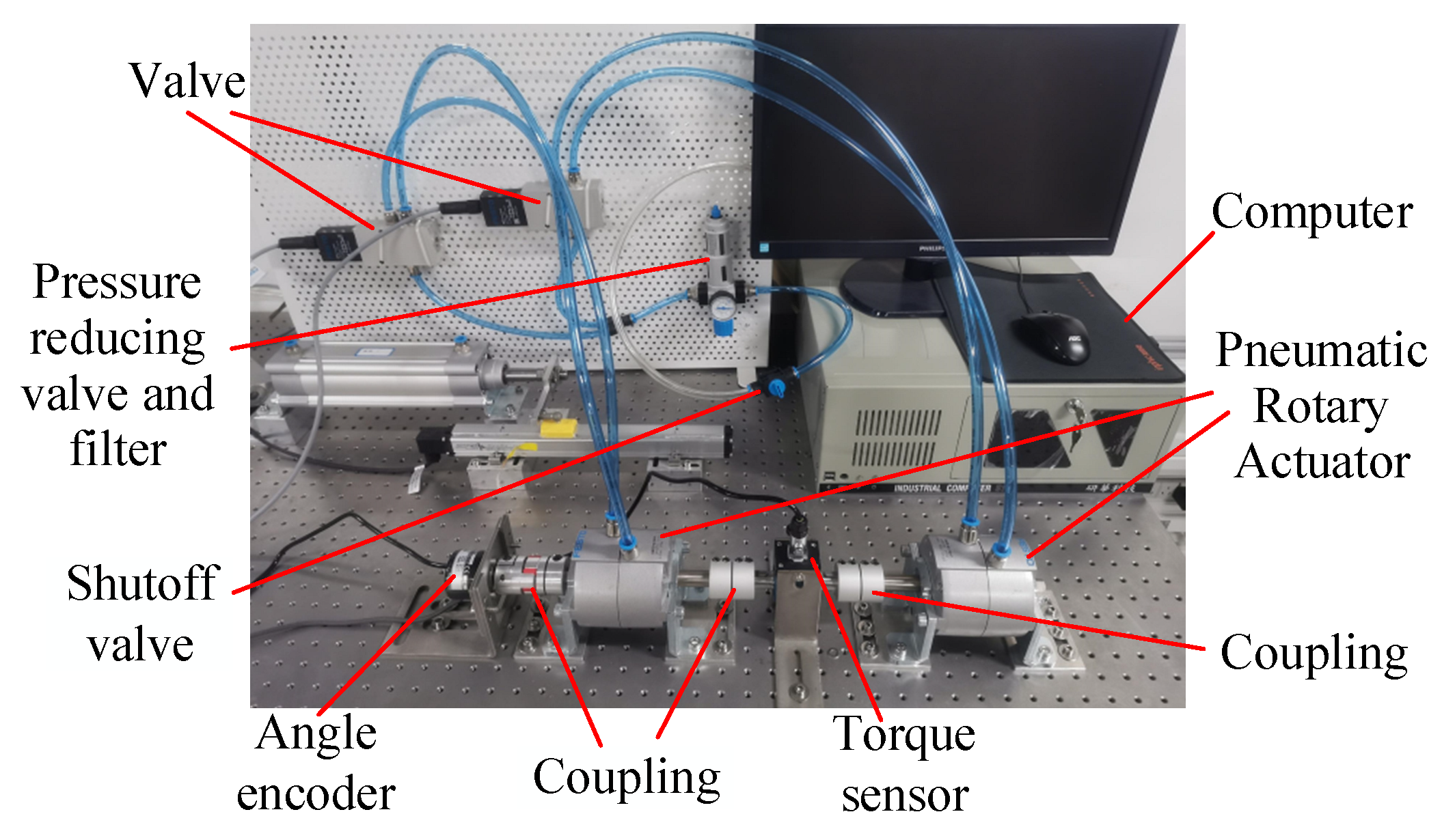
The execution device comprises two pneumatic rotary actuators (Festo, Esslingen, Germany, DRVS-40-180-P). This system is also equipped with an angle encoder (OMRON-E6C3-A), a torque sensor (QLN-10 (10–100 Nm)), and two proportional valves (Festo, MPYE-5-1/4-010-B). In addition to these devices, there is also an industrial computer (Advantech, Taiwan, China, 510H), two data-acquisition cards (Advantech, PCI-1716, and PCI-1784), and a D/A card (Advantech, PCI-1723). The parameters of the system are shown in Table 1.

Table 1.
Parameters of the system.
2.2. Dynamic Model
To simplify the mathematical model appropriately, the following assumptions have been made [8]:
- (1)
- The gas in the system follows the ideal gas equation of state.
- (2)
- The flow of gas is assumed to be an isentropic process.
- (3)
- There is no effect of piping on air-pressure transfer.
- (4)
- The gas temperature remains constant during the flow.
- (5)
- The actuator and the outside world, as well as between the two chambers, have no leakage.
To simplify the modeling complexity, the valve is approximated by a first-order model as presented below:
where and are coefficients to be determined. is the effective cross-sectional area of the proportional servo valve orifice, while is the control variable.
The gas-flow equation through the valve port can be obtained from the above assumptions as follows:
where is the flow function of gas passing through a small hole, and is the mass-flow rate passing through the valve. , , and are the flow coefficient, diabatic index of the gas, and gas temperature, respectively. and are the pressures of the inflowing and outflowing gas, respectively.
The expression for the ideal gas-state equation is as follows:
Differentiating both sides of Equation (4):
where is the gas pressure, is the gas density, is the ideal gas constant, and is the temperature.
The mass-flow equation is as follows:
where and represent the mass-flow rates into and out of the pneumatic rotary actuator, respectively.
Substituting Equation (8) into Equation (5) yields the pressure-differential equation inside the pneumatic rotary actuator:
where and represent the total volume and internal pressure of the pneumatic rotary actuator, respectively.
where
is the effective area of the fan blade, and
and
are the ineffective volume and rotation angle.
where is the system output torque, and is the displacement of the pneumatic rotary actuator, respectively.
The simplified second-order model of the torque control system is as follows:
Differentiating and transforming Equation (4) into a normalized form of the equation of state:
where and denote torque, while represents the derivative of the torque.
Let
where is a gain variable adjusted based on the system inertia to compensate for the system total nonlinearity, is the control voltage generated by the controller, is the total nonlinearity of the pneumatic-torque servo system, and .
2.3. Design of an Active Disturbance-Rejection Controller Integrated with a Kalman Filter
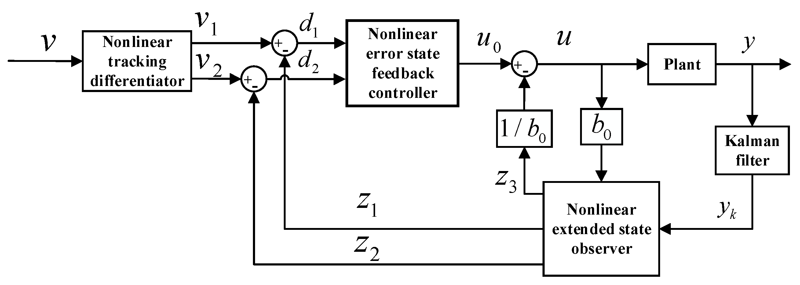
This paper presents an active disturbance-rejection torque controller integrated with a Kalman filter (ADRCKF) to enhance the torque control precision of a pneumatic rotary actuator. The algorithm diagram of the ADRCKF is presented in Figure 2.
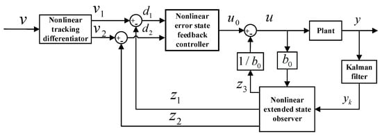
Figure 2.
Algorithm diagram of the active disturbance-rejection torque controller integrated with a Kalman filter.
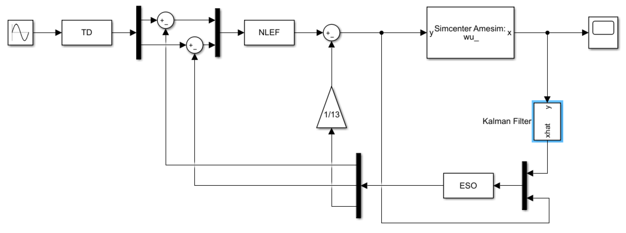
The algorithm in Figure 2 is explained as follows: The feedback value is transmitted to a Kalman filter to generate the signal . , along with the control input multiplied by the gain , is input into the nonlinear extended-state observer to generate the observed value of , as well as the first derivative and the second derivative of the observed value . The desired signal is conveyed to a nonlinear tracking differentiator to generate the transitional signal of the desired signal and its derivative . is obtained by taking the difference between and , and is obtained by taking the difference between and . and are input into the nonlinear error-state feedback controller to generate the control signal . The final control signal is obtained by subtracting the nonlinear compensation term from , and is passed to the control object to produce the output .
2.3.1. Kalman Filter
The Kalman filter is a powerful tool for estimating system states and has gained widespread popularity across different domains, mainly due to its ability to accurately estimate system states even in the presence of uncertainties and noise. The Kalman filter is proposed to perform real-time filtering of signals fed back to the nonlinear extended-state observer (ESO), improving the observation accuracy of the ESO and effectively suppressing the chatter caused by noise signals.
For discrete systems:
where represents the process noise signal, and represents the measurement noise signal.
The discrete formula of the first-order Kalman filter recursive algorithm is presented below:
The estimation error is characterized by the following covariance:
The parameters , , , , and are all variables that can be adjusted to achieve the desired filtering behavior. For instance, the balance between the influence of process noise and measurement noise on the filter is determined by the values of the covariance matrices and ; these, therefore, influence the ability of the filter to accurately estimate the system state. Similarly, the parameters , , and affect the propagation of the state estimate over time and, therefore, the response of the filter to changes in the system dynamics. By properly adjusting these parameters, the Kalman filter can be optimized for a particular system and improve its accuracy and efficiency. In this paper, , , , , , .
2.3.2. Nonlinear Tracking Differentiator
The purpose of designing the nonlinear tracking differentiator (TD) in this article is to arrange the transition process and generate a smooth and continuous signal of the input signal and its differential signal. The nonlinear function is proposed for filtering and fast-tracking. Let ; then, a second-order TD is designed as follows:
where is an error between a transition signal and a desired input signal. , , and represent the desired input signals, the smoothed transition signal of the input signal , and the derivative signal of the transition signal , respectively. The expression for the function is as follows:
where , , , .
where the parameters , and are all positive real numbers, represents the filtering factor, and represents the sampling step. The response speed of the transient process is able to be adjusted by modifying the value of . In practice, the adopted step size is set larger than to prevent overshooting.
2.3.3. Nonlinear Extended-State Observer
To address dynamic external disturbances and internal nonlinearity, a nonlinear extended-state observer (ESO) is introduced to perform real-time estimation of the internal nonlinearity and dynamic external disturbances within the torque system and to expand them into total nonlinearity for real-time compensation. The total nonlinearity is expanded into a new state variable ; . The pneumatic-torque servo control system (15) is extended as follows:
where is the derivative of . In practice, is delimited. Defining and , the expression for the second-order ESO is as follows:
where is the observed value of for . In addition, the performance of the ESO can be adjusted by tuning the three gains , , and . The nonlinear function is proposed to reduce signal oscillation. The nonlinear function is given by the following expression:
where and are two given positive parameters, and is the error value. The parameter is a value constrained within a specified range: . Parameter is the sampling step-size of the function, and tuning both and adjusts the performance of the function.
Remark 1.
The saturation function is a monotonically smooth, continuously increasing odd function. However, it is not smooth and not differentiable at .
According to Formulas (26) and (27), the error equations of ESO are as follows:
where ; .
The self-stabilizing region method has been employed to prove the convergence of the system (29), as in [26,27,28]. However, this method is considered too intricate. In this paper, the Lyapunov function is proposed to demonstrate the convergence of the ESO.
Theorem 1.
If Lyapunov-like lemma
then .
Proof.
The design of the Lyapunov function is as follows:
where is delimited in practice, such as in [29,30,31]. There exist parameters , , and that are sufficiently large to satisfy . The effectiveness of the ESO has been demonstrated, leading to the convergence of the observed values of , , and to , , and , respectively.
When , the derivative of the function does not exist. This is because when , the left and right derivatives are not equal, but both its left and right derivatives exist and are bounded. Therefore, when , the derivation is based on , and when , the derivation is based on , which still satisfies the above analysis of . □
2.3.4. Nonlinear Error-State Feedback Controller
The following equations define the error signals between a tracking differentiator and an extended-state observer:
where and represent the torque and its differential signal, respectively, while and denote the corresponding observation output signals.
The controlled variable of the following is the formulation of the nonlinear error-state feedback controller (NLEF):
where and are two control gains, while represents the compensation for the system (15) nonlinearity.
The errors between the input and output signals are as follows:
By incorporating system (15) into system (33), the error system is redefined:
where denotes the derivative of , which is both continuous and delimited.
By combining Equations (30) and (33), we obtain:
To simplify the expression, we denote as and as . Furthermore, by using Equations (26) and (34), we have:
Theorem 2.
By selecting appropriate gain variables and , the nonlinear error-state feedback controller (32) is stable and convergent, and the error system (34) is also convergent, resulting in the convergence of the output signals and to and , respectively.
In [32], examples of stability analysis for data-driven controllers are presented. This study employs the Lyapunov stability theory for the stability analysis of the controller.
Proof.
Let the Lyapunov function be designed as:
The derivative of is given by:
Setting
We have
From (35), we have
is an odd function and monotonically increasing. To simplify the analysis, let . The analysis is then as follows:
- (1)
- If then
- (2)
- If then
Therefore, the conclusion is as follows:
The boundedness of , , and is guaranteed by the proven convergence of the ESO. Additionally, , , and are also bounded.
Letting
obviously, H is also bounded.
There exist sufficiently large values of and such that there exists a region where holds. According to the proof provided above, it can be inferred that the stability of the closed-loop system (34) can be guaranteed by judicious selection of the parameters and in the ADRCKF. □
3. Results
3.1. Simulation Result
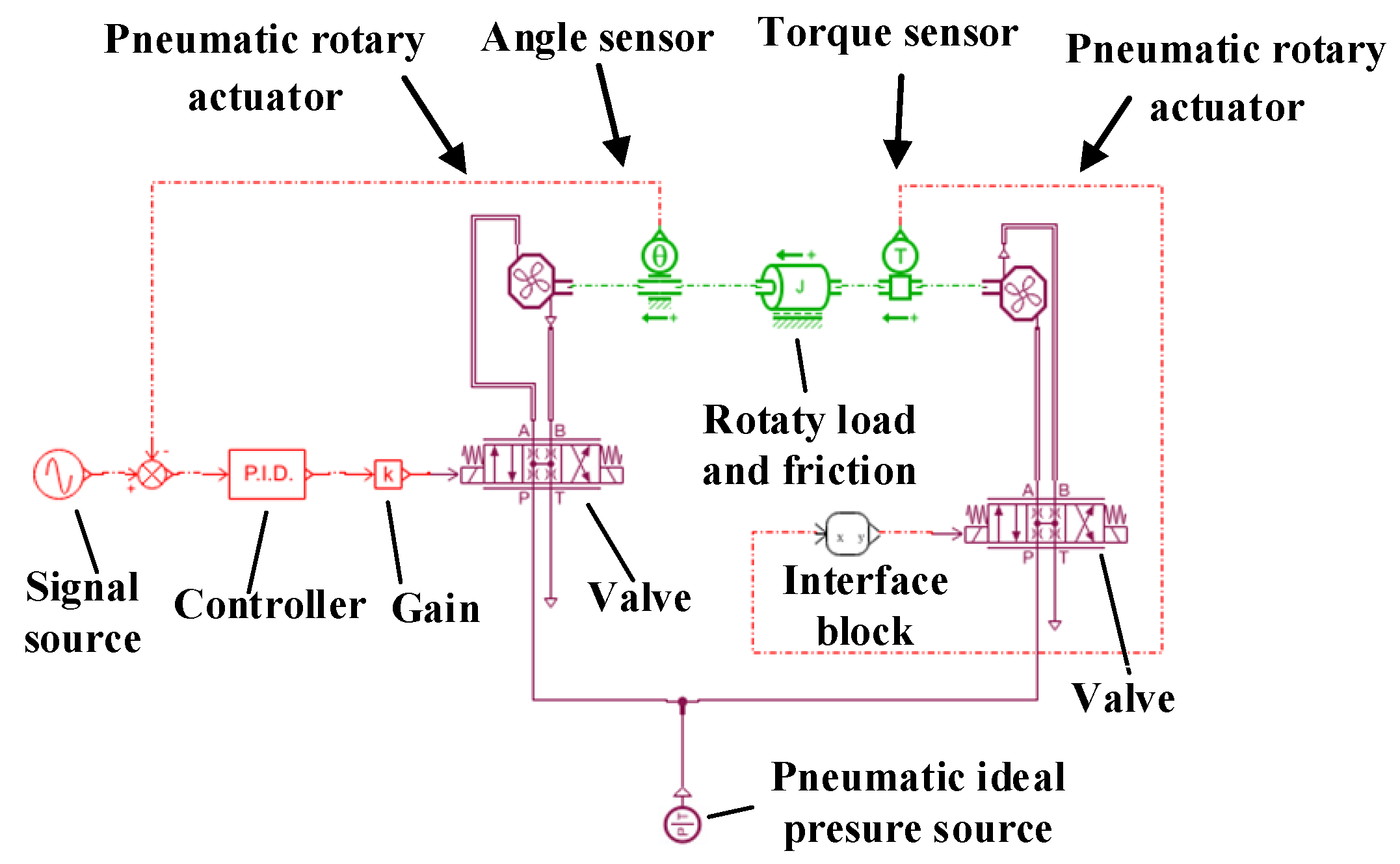
This study utilizes Amesim and Simulink for combined simulation to validate the feasibility of the algorithm. The physical model designed in Amesim is depicted in Figure 3, while the mathematical model of the algorithm designed in Simulink is presented in Figure 4.
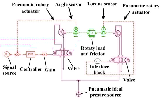
Figure 3.
The physical model designed in Amesim.
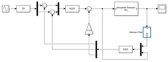
Figure 4.
The mathematical model of the algorithm designed in Simulink.
The specific working principles are explained using the active disturbance-rejection controller with integrated Kalman filter (ADRCKF) as an example. The angle sensor in Figure 3 captures the actual output angle and the expected angle signal and calculates the difference to obtain the error, which is then input into the PID controller to obtain the control quantity. The control quantity is multiplied by a gain to generate a control voltage that is input to the valve. The control voltage regulates the opening area of the valve interface, controlling gas flow. Changes in flow impact the position output, achieving closed-loop control of the position. This constitutes the position-disturbance control part on the position side. The position disturbance is applied to the torque control part, introducing an additional position disturbance. The primary objective of this paper is to achieve precise torque control under external position disturbance. The control principle on the torque side is as follows: The torque sensor in Figure 3 captures the actual torque output signal, which is then transmitted to the Interface block. The Interface block, through the control Simulink algorithm in Figure 4, generates a control quantity that is transferred to the valve. By controlling the voltage of the valve, the opening area of the valve is regulated, achieving flow control. Changes in flow influence the torque output, realizing closed-loop control of torque. The algorithm principles in Figure 4 were already explained when introducing Figure 2 and will not be reiterated here.
Due to the interference of the position system with the torque system, oscillations occur in the torque system, particularly at the reversal point, as illustrated in the simulation results in Figure 5a,c. The research challenge addressed in this study revolves around mitigating the adverse effects caused by the interference of the position system with the torque system, with the aim of achieving precise torque control.
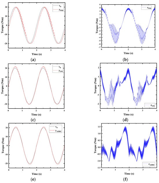
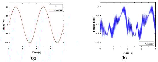
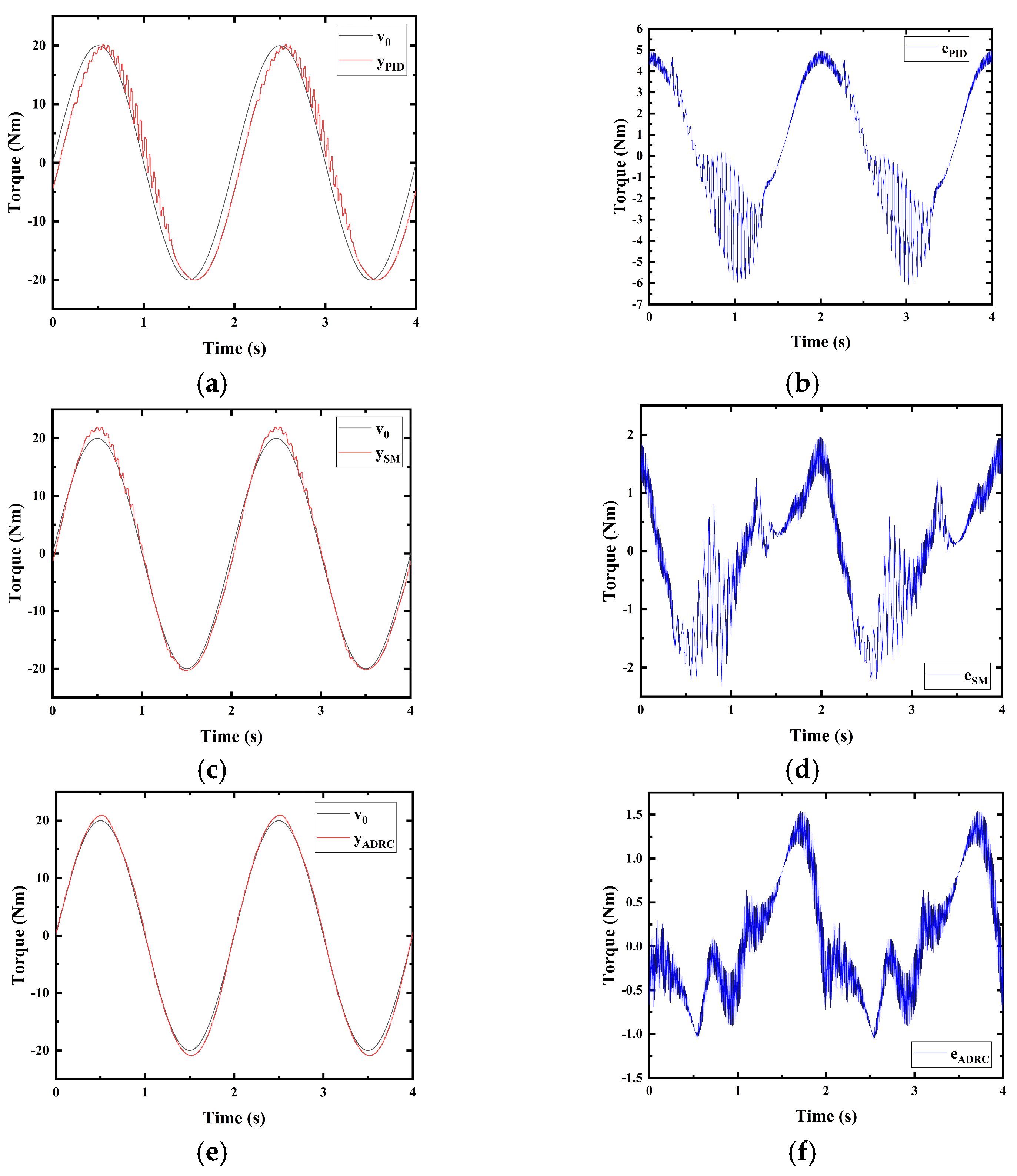
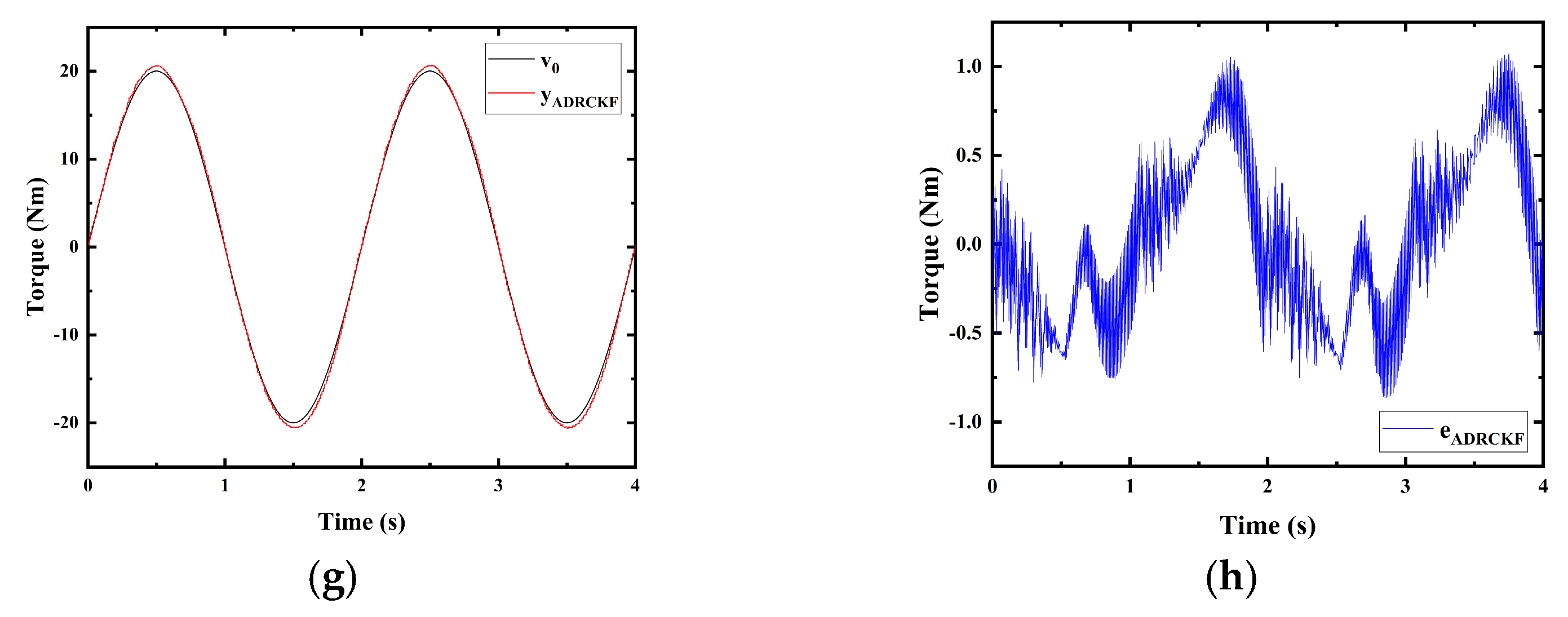
Figure 5.
Simulation results of torque control under position disturbance were obtained using a PID, an SM, an ADRC, and an ADRCKF at a frequency of 0.5 Hz. (a) Torque trajectory tracking of the PID. (b) Torque trajectory−tracking error of the PID. (c) Torque trajectory tracking of the SM. (d) Torque trajectory−tracking error of the SM. (e) Torque trajectory tracking of the ADRC. (f) Torque trajectory−tracking error of the ADRC. (g) Torque trajectory tracking of the ADRCKF. (h) Torque trajectory-tracking error of the ADRCFK.
The paper presents a simulation comparison of a PID, an SM, an ADRC, and an ADRCKF controller with an amplitude of 20 Nm and a frequency of 0.5 Hz, as depicted in Figure 5. Figure 5a depicts the simulation results of PID torque trajectory tracking, which shows evident oscillations. The PID controller lacks disturbance-rejection capability, leading to significant oscillations at the reversal point of the torque signal due to interference from the position system. Figure 5b represents the torque trajectory-tracking error for PID, with a maximum error of 6 Nm. Figure 5c illustrates the simulation results of SM torque trajectory tracking, displaying slight oscillations. The disturbance-rejection capability of the sliding-mode controller is slightly superior to that of PID, consequently leading to a reduced magnitude of oscillations compared with PID. Figure 5d shows the torque trajectory-tracking error for SM, with a maximum error of 2.3 Nm. Figure 5e displays the simulation results of ADRC torque trajectory tracking, without oscillations. Owing to the strong disturbance-rejection capability and robustness of the active disturbance-rejection controller, oscillations are virtually eliminated. Figure 5f presents the torque trajectory tracking error for the ADRC, with a maximum error of 1.6 Nm. Figure 5g shows the simulation results of the ADRCKF torque trajectory tracking. The ADRCKF exhibits superior disturbance-rejection capability and robustness; oscillations are completely eliminated, and the output signal closely adheres to the desired signal. Figure 5h represents the torque trajectory-tracking error for the ADRCKF, with a maximum error of 1.1 Nm. Note that 1.1 Nm < 1.6 Nm < 2.3 Nm < 6 Nm. The simulation results validate the effectiveness and superiority of the ADRCFK control strategy.
The maximum errors of PID, SM, ADRC, and ADRCKF controllers in simulating sinusoidal-torque trajectory tracking with an amplitude of 20 Nm and a frequency of 0.5 Hz are presented in Table 2.
Table 2.
Simulation results at 0.5 Hz.
3.2. Experimental Results
The experimental setup examined in this research is a pneumatic-torque system that is based on position disturbance, and it is illustrated in Figure 6.
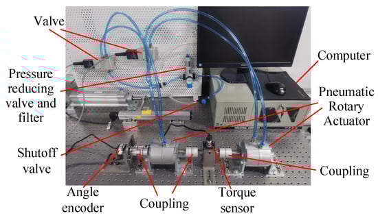
Figure 6.
Experimental setup with two pneumatic rotary actuators.
Using an experimental air-pressure condition of 0.7 MPa, an experiment was conducted to measure the dead zone of the proportional valve, which was found to be between 4.9 V and 5.1 V. The following parameters were used to design the ADRCKF:
For different experiments, the parameters were set differently. For the sinusoidal-torque trajectory tracking at a frequency of 0.5 Hz, , and . For the 1 Hz sinusoidal-torque trajectory tracking, , and .
In the presence of position disturbance with a frequency of 0.5 Hz and an amplitude of 85°, the PID controller conducted a sinusoidal-torque trajectory tracking experiment with a frequency of 0.5 Hz and an amplitude of 20 Nm, as illustrated in Figure 7. The active disturbance-rejection controller (ADRC), the active disturbance-rejection controller integrated with a Kalman filter (ADRCKF), and the sliding-mode controller (SM) performed a sinusoidal-torque trajectory-tracking experiment with a frequency of 0.5 Hz and an amplitude of 20 Nm, as shown in Figure 8. Under the conditions of position disturbance with a frequency of 1 Hz and an amplitude of 85°, the ADRC, ADRCKF, and SM conducted sinusoidal-torque tracking experiments with a frequency of 1 Hz and an amplitude of 20 Nm, as presented in Figure 9.
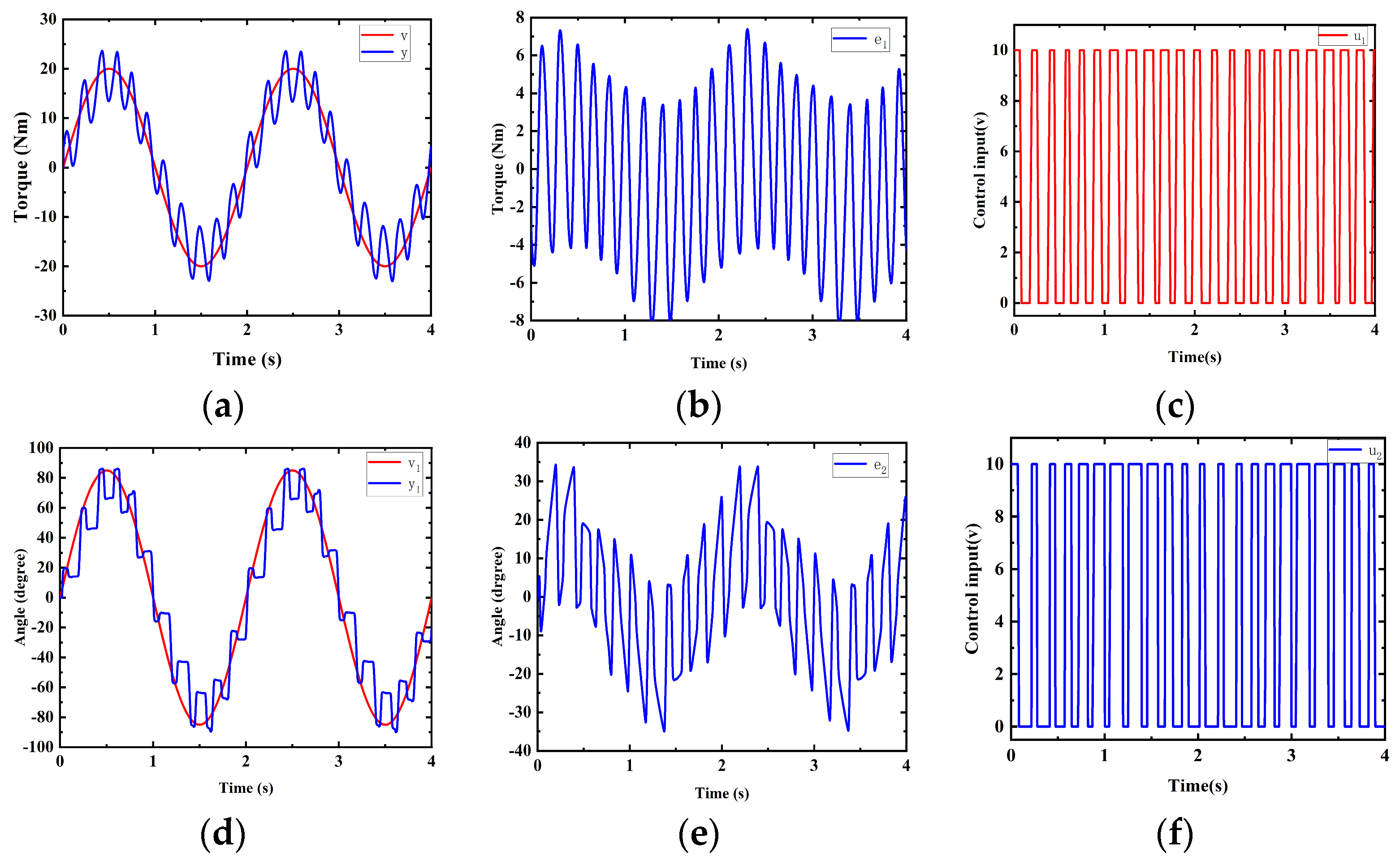
Figure 7.
Experimental results of a torque control based on position disturbance, controlled by a PID controller at a frequency of 0.5 Hz. (a) Torque. (b) Torque error. (c) Control input of the torque system. (d) Angle. (e) Angle error. (f) Control input of the position system.
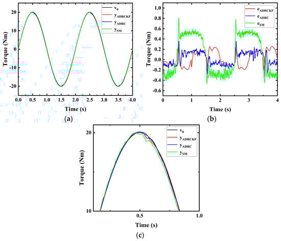
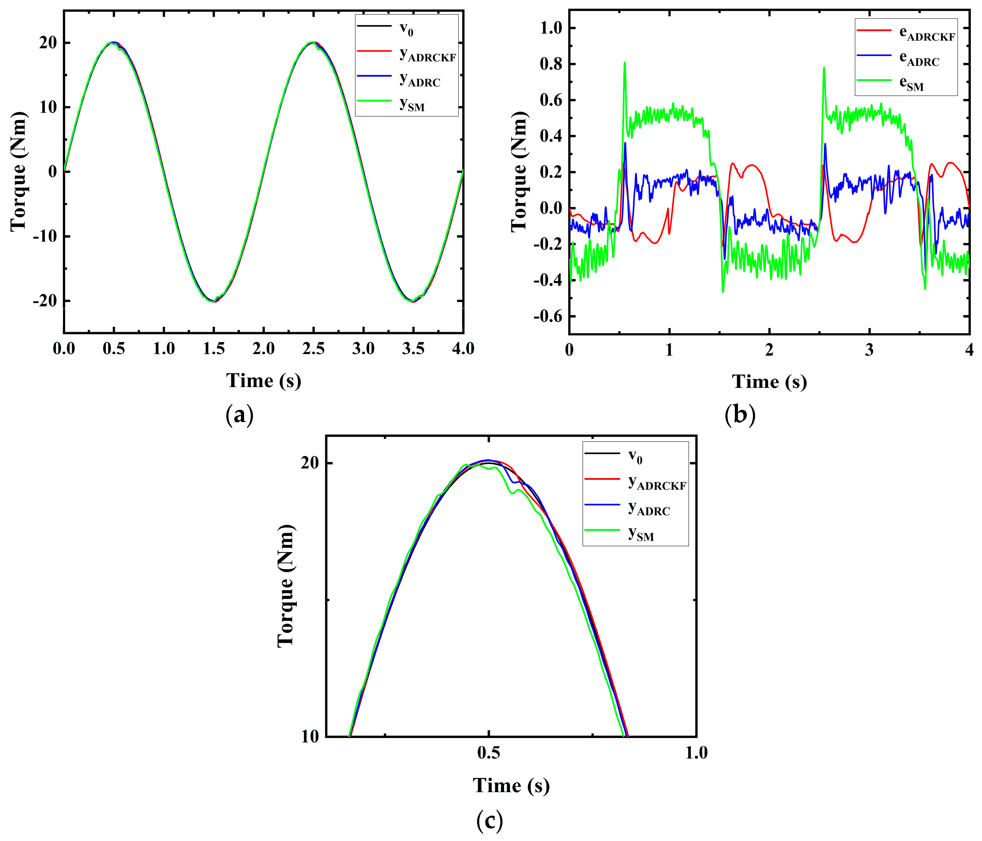
Figure 8.
Experimental results of torque control under position disturbance were obtained using an ADRCKF, an ADRC, and an SM at a frequency of 0.5 Hz. (a) Torque trajectory tracking. (b) Torque trajectory−tracking error. (c) Partial enlarged drawing of the ADRCKF, ADRC, and SM.
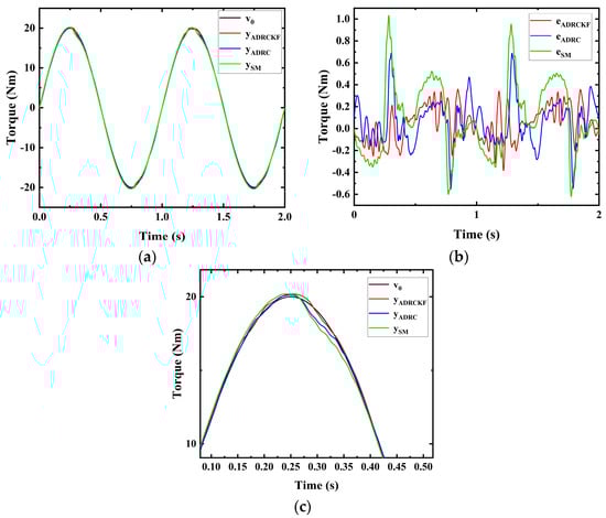
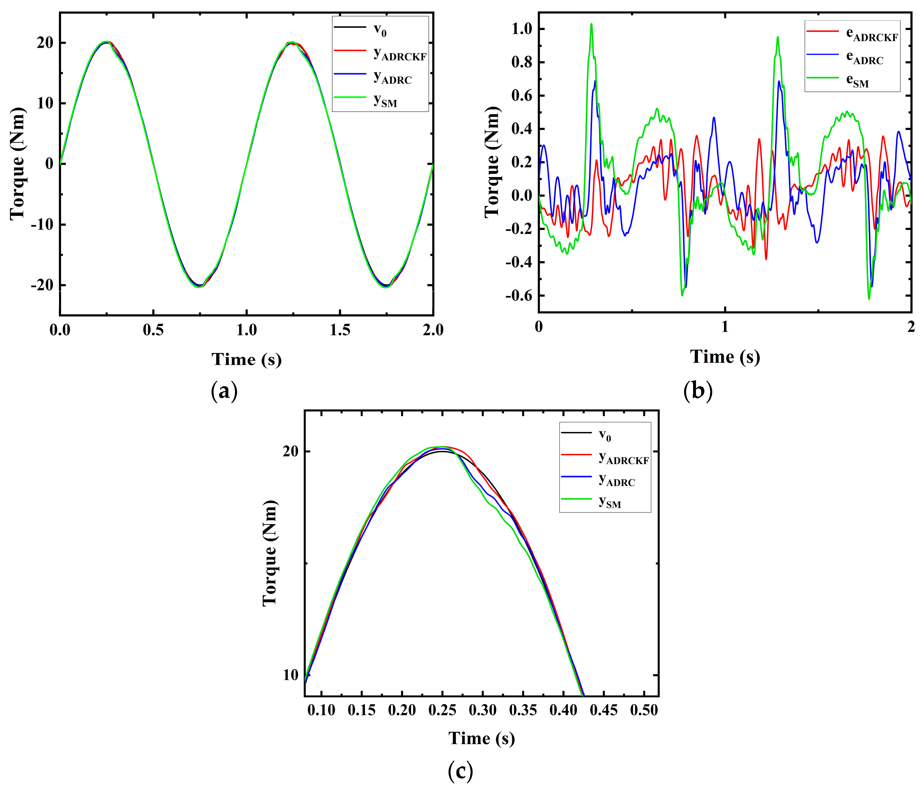
Figure 9.
Experimental results of torque control under position disturbance were obtained using an ADRCKF, an ADRC, and an SM at a frequency of 1 Hz. (a) Torque trajectory tracking. (b) Torque trajectory−tracking error. (c) Partial enlarged drawing of the ADRCKF, ADRC, and SM.
Figure 7 illustrates experiments of a pneumatic-torque servo control controlled by a PID controller that is based on position disturbance. The position disturbance signal is a sinusoidal signal with an amplitude of 85° and a frequency of 0.5 Hz. The torque signal to be controlled is a sinusoidal signal with an amplitude of 20 Nm and a frequency of 0.5 Hz. Figure 7a,d, respectively, show the output of torque trajectory tracking and the angle output of the position-disturbance part. Figure 7b,e show the corresponding tracking errors and , which are 8 Nm and 35 degrees, respectively. Figure 7a,d exhibit significant oscillations. This is attributed to the poor robustness of the PID controller and the series connection of the position output terminal and the torque output terminal, leading to mutual interference. Figure 7c,f display the control voltage and of the valve in the torque and position systems, respectively. It can be observed that the voltage of both valves reached the limit, indicating that the valves are operating at their optimal performance. This results in the system control accuracy being at its highest level.
Figure 8 depicts the experiments of sinusoidal-torque trajectory tracking based on position disturbances. The controlled torque signal is a sinusoidal signal with an amplitude of 20 Nm and a frequency of 0.5 Hz, while the position disturbance signal is a sinusoidal signal with an amplitude of 85° and a frequency of 0.5 Hz. Figure 8a illustrates the sinusoidal-torque trajectory-tracking experiment controlled by an ADRCKF, an ADRC, and an SM, where the output signals , , and rapidly track the desired torque signal . Figure 8b represents the tracking errors in the sinusoidal-torque trajectory controlled by the ADRC, ADRCKF, and SM, with maximum tracking errors of 0.25 Nm, 0.38 Nm, and 0.8 Nm for , , and , respectively. Note that 0.25 Nm < 0.38 Nm < 0.8 Nm < 8 Nm. Figure 8c shows a comparatively enlarged view of the ADRCKF, ADRC, and SM under position disturbances during the sinusoidal-torque trajectory-tracking experiment. At the commutation point, the outputs , , and of the three controllers both oscillated, but the ADRCKF was less affected by oscillations, resulting in higher control accuracy. This indicates that the Kalman filter effectively enhances system robustness and suppresses system oscillations.
Figure 9 depicts experiments of a pneumatic-torque servo control based on position disturbance, controlled by an ADRCKF, an ADRC, and an SM. The controlled torque signal is a sinusoidal signal with an amplitude of 20 Nm and a frequency of 1 Hz, while the position disturbance signal is a sinusoidal signal with an amplitude of 85° and a frequency of 1 Hz. In Figure 9a, the sinusoidal-torque tracking experiment controlled by an ADRCKF, an ADRC, and an SM is depicted, with the output signals , , and rapidly tracking the desired torque signals. In Figure 9b, the sinusoidal-torque trajectory-tracking errors controlled by the ADRCKF, ADRC, and SM are shown, with maximum tracking errors of 0.4 Nm, 0.7 Nm, and 1.0 Nm for , , and , respectively. Note that 0.4 Nm < 0.7 Nm < 1.0 Nm. The experiment once again demonstrates the superior performance of the ADRCKF.
This paper, under the condition of position disturbance with a frequency of 0.5 Hz and an amplitude of 85°, designed three sets of experiments for tracking sinusoidal-torque trajectories with a frequency of 0.5 Hz and an amplitude of 20 Nm for comparison. The four controllers used were the PID, ADRCKF, ADRC, and SM. The tracking errors for the four sets of experiments are shown in Figure 7b and Figure 8b, which are 8 Nm, 0.25 Nm, 0.36 Nm, and 0.8 Nm, respectively. Additionally, it explored the tracking of a sinusoidal torque with a frequency of 1 Hz and an amplitude of 20 Nm using an ADRCKF, an ADRC and an SM under the condition of position disturbance with a frequency of 1 Hz and an amplitude of 85°, as illustrated in Figure 9a. The tracking errors are 0.4 Nm, 0.7 Nm, and 1.0 Nm respectively, as shown in Figure 9b.
The maximum errors in the results of the 0.5 Hz sinusoidal-torque tracking experiments under different control strategies are shown in Table 3, while the maximum errors in the results of the 1 Hz sinusoidal-torque tracking experiments under different control strategies are presented in Table 4.
Table 3.
0.5 Hz experimental results.
Table 4.
1 Hz experimental results.
In addition to utilizing the maximum-error metric, the integral absolute-error metric (IAE) is also employed. Over a specified time period, the absolute values of errors for various controllers are integrated to derive the IAE metrics. The IAE metrics for the 0.5 Hz sine experiment are presented in Table 5, while the IAE metrics for the 1 Hz sine experiment are detailed in Table 6.
Table 5.
0.5 Hz experimental results.
Table 6.
1 Hz experimental results.
Remark 2.
Sinusoidal-torque trajectory tracking based on position disturbance shows the poor performance of the PID controller. This is because the position output and torque output interfere with each other, and the PID controller lacks robustness, making the torque-control part unable to resist interference from the position side. In contrast, the SM, the ADRC, and the ADRCKF controllers demonstrate strong robustness and high disturbance-rejection capabilities, leading to more satisfactory torque trajectory-tracking control. However, integrating the Kalman filter into the ADRC controller improves the purity of the feedback signal, increases the robustness of the controller, reduces oscillations, and enhances control precision.
4. Discussion
This paper employs an active disturbance-rejection controller integrated with a Kalman filter to suppress system oscillations, achieving precise torque control. In comparison with the four data-driven control methods mentioned in the introduction, it exhibits superior disturbance-rejection capabilities and higher real-time performance. This is attributed to the real-time estimation and compensation of internal nonlinearity and external disturbances by the nonlinear extended observer, thereby offsetting both internal nonlinearity and external disturbances. Additionally, the Kalman filter performs state estimation on the system and filters the feedback signals, enhancing the robustness of the system. In the context of data-driven methodologies, the present application of the ADRCKF entails feedback control that relies on real-time input, output, and estimated disturbance value.
The primary challenge in the control methodology presented in this paper lies in the mutual interference and coupling between the torque and position systems. As depicted in Figure 8b and Figure 9b, the maximum error manifests after the reversal point. Both the torque signal and the position signal are sinusoidal signals with identical frequencies. When the torque signal reverses, the position signal also reverses simultaneously. At this juncture, the acceleration of the position system is maximal, resulting in the most substantial torque disturbance to the torque system. Consequently, the largest error in the torque system emerges after the reversal point.
In Figure 7, the experimental setup employed a PID controller, resulting in pronounced system oscillations. This is attributed to the limited robustness of the PID controller, which hinders its ability to effectively counteract external position disturbances. Experiment 8 utilized a sliding-mode controller based on the extended observer from the literature [11], an ADRC, and an ADRCKF. At the reversal point, the ADRCKF experienced the least impact, resulting in the smallest maximum error. As shown in Table 3, the minimum error for the ADRCKF was 0.25 Nm. Similarly, in Experiment 9, the ADRCKF encountered minimal influence at the reversal point, leading to the smallest maximum error. As indicated in Table 4, the minimum error for the ADRCKF was 0.4 Nm. Furthermore, the IAE results in Table 5 and Table 6 confirm that the ADRCKF exhibits stronger disturbance-rejection capabilities compared with the ADRC and SM. The experimental results indicate that the improvement of the active disturbance-rejection controller through the integration of a Kalman filter is effective. It successfully suppressed system oscillations, enhancing the resistance to disturbances of the system and overall robustness. In the future, it is anticipated to achieve better application performance in systems with strong disturbances.
5. Conclusions
This paper presented an ADRCKF for the pneumatic-torque servo control system based on positional interference. This approach has proven to be an effective means of mitigating nonlinearity and disturbances in pneumatic-torque servo systems. The Kalman filter enhances the purity of the feedback signal in real-time, effectively reduces oscillation, and improves control accuracy. The total nonlinearity in the pneumatic servo system is estimated and compensated for in real time by the ESO, which then feeds back all observed values to the nonlinear error-state feedback controller (NLEF). The Lyapunov stability theory is utilized to demonstrate the validity of the ESO and the convergence of the NLEF. Experimental results confirm the excellent performance of the ADRCKF. For sinusoidal signal tracking with a 0.5 Hz amplitude of 20 Nm, the torque error is within 0.25 Nm. Similarly, at a corresponding frequency of 1 Hz, the torque error is within 0.4 Nm. However, there is still room for improvement, particularly regarding the precision of high-frequency control.
Author Contributions
Conceptualization and writing—original draft preparation, Z.W.; methodology and software, Z.W.; review and editing, Q.W.; data processing, D.K. and Y.Z.; supervision, D.Z. All authors have read and agreed to the published version of the manuscript.
Funding
This research was supported by the National Natural Science Foundation of China (Grant number 51905159) and the National Natural Science Foundation of China (Grant number 52075152).
Data Availability Statement
Data are contained within the article.
Conflicts of Interest
The authors declare no conflicts of interest.
References
- Schluter, M.; Perondi, E. Mathematical Modeling with Friction of a SCARA Robot Driven by Pneumatic Semi-rotary Actuators. IEEE Lat. Am. Trans. 2020, 18, 1066–1076. [Google Scholar] [CrossRef]
- Khin, M.; Low, H. Shape Programming Using Triangular and Rectangular Soft Robot Primitives. Micromachines 2019, 10, 236. [Google Scholar] [CrossRef]
- Fan, C.; Hong, G.S.; Zhao, J.; Zhang, L.; Zhao, J.; Sun, L.N. The integral sliding mode control of a pneumatic force servo for the polishing process. Precis. Eng. 2019, 55, 154–170. [Google Scholar] [CrossRef]
- Saravanakumar, D.; Mohan, B.; Muthuramalingam, T. A review on recent research trends in servo pneumatic positioning systems. Precis. Eng. 2017, 49, 481–492. [Google Scholar] [CrossRef]
- Saravanakumar, D.; Mohan, B.; Muthuramalingam, T.; Sakthivel, G. Performance evaluation of interconnected pneumatic cylinders positioning system. Sens. Actuators A—Phys. 2018, 274, 155–164. [Google Scholar]
- Aziz, M.A.; Benini, E.; Elsayed, M.E.A.; Khalifa, M.A.; Gaheen, O.A. Speed and torque control of pneumatic motors using controlled pulsating flow. Int. J. Adv. Manuf. Technol. 2023, 127, 635–648. [Google Scholar] [CrossRef]
- Wei, Q.; Jiao, Z.; Wang, J. Control of Pneumatic Position Servo with LuGre Model-based Friction Compensation. J. Mech. Eng. 2018, 54, 131–138. [Google Scholar] [CrossRef]
- Wei, Q.; Jiao, Z.; Wu, S. Nonlinear Compound Control of Pneumatic Servo Loading System. J. Mech. Eng. 2017, 53, 217–224. [Google Scholar] [CrossRef]
- Ruihua, L.; Guoxiang, M.; Zhengjin, F.; Yijie, L.; Weixiang, S. A Sliding Mode Variable Structure Control Approach for a Pneumatic Force Servo System. In Proceedings of the 2006 6th World Congress on Intelligent Control and Automation, Dalian, China, 21–23 June 2006; Volume 2, pp. 8173–8177. [Google Scholar]
- Zhao, L.; Zhang, B.; Yang, H.J.; Wang, Y.J. Observer-Based Integral Sliding Mode Tracking Control for a Pneumatic Cylinder with Varying Loads. IEEE Trans. Syst. Man Cybern. Syst. 2020, 50, 2650–2658. [Google Scholar] [CrossRef]
- Wang, T.; Chen, X.X.; Qin, W. A novel adaptive control for reaching movements of an anthropomorphic arm driven by pneumatic artificial muscles. Appl. Soft Comput. 2019, 83, 105623. [Google Scholar] [CrossRef]
- Taheri, B.; Case, D.; Richer, E. Force and Stiffness Backstepping-Sliding Mode Controller for Pneumatic Cylinders. IEEE/ASME Trans. Mechatron. 2014, 19, 1799–1809. [Google Scholar] [CrossRef]
- Meng, D.Y.; Tao, G.L.; Ban, W.; Qian, P.F. Adaptive robust output force tracking control of pneumatic cylinder while maximizing/minimizing its stiffness. J. Cent. South Univ. 2013, 20, 1510–1518. [Google Scholar] [CrossRef]
- Bobrow, J.E.; Jabbari, F. Adaptive pneumatic force actuation and position control. J. Dyn. Syst. Meas. Control 1991, 113, 267–272. [Google Scholar] [CrossRef]
- Fan, C.; Xue, C.; Zhang, L.; Wang, K.; Wang, Q.; Gao, Y.; Lu, L. Design and control of the belt-polishing tool system for the blisk finishing process. Mech. Sci. 2021, 12, 237–248. [Google Scholar] [CrossRef]
- Precup, R.-E.; Preitl, S.; Rudas, I.J.; Tomescu, M.L.; Tar, J.K. Design and experiments for a class of fuzzy controlled servo systems. IEEE/ASME Trans. Mechatron. 2008, 13, 22–35. [Google Scholar] [CrossRef]
- Roman, R.C.; Precup, R.E.; Hedrea, E.L.; Preitl, S.; Zamfirache, I.A.; Bojan-Dragos, C.A.; Petriu, E.M. Iterative feedback tuning algorithm for tower crane systems. Procedia Comput. Sci. 2022, 199, 157–165. [Google Scholar] [CrossRef]
- Gao, S.L.; Zhao, D.Y.; Yan, X.G.; Spurgeon, S.K. Model-Free Adaptive State Feedback Control for a Class of Nonlinear Systems. In IEEE Transactions on Automation Science and Engineering; IEEE: Piscataway, NJ, USA, 2023. [Google Scholar]
- Liu, B.; Jin, Y.; Zhu, C.; Chen, C. Pitching axis control for a satellite camera based on a novel active disturbance rejection controller. Adv. Mech. Eng. 2017, 9, 1687814016689039. [Google Scholar] [CrossRef]
- Tan, L.; Liang, S.; Su, H.; Qin, Z.; Li, L.; Huo, J. Research on Amphibious Multi-Rotor UAV Out-of-Water Control Based on ADRC. Appl. Sci. 2023, 13, 4900. [Google Scholar] [CrossRef]
- Huang, Y.; Xue, W. Active disturbance rejection control: Methodology and theoretical analysis. ISA Trans. 2014, 53, 963–976. [Google Scholar] [CrossRef]
- Han, J. From PID to active disturbance rejection control. IEEE Trans. Ind. Electron. 2009, 56, 900–906. [Google Scholar] [CrossRef]
- Li, J.; Qi, X.; Wan, H.; Xia, Y. Active disturbance rejection control:theoretical results summary and future researches. Control Theory Appl. 2017, 34, 281–295. [Google Scholar]
- Sun, M.; Jiao, G.; Yang, R.; Chen, Z. Application and analysis of ADRC in guidance and control in flight vehicle—Some explorations in various time-scale paradigms. In Proceedings of the 29th Chinese Control Conference, Beijing, China, 20 September 2010; pp. 6167–6172. [Google Scholar]
- Stojanovic, V.; He, S.P.; Zhang, B.Y. State and parameter joint estimation of linear stochastic systems in presence of faults and non-Gaussiannoises. Int. J. Robust Nonlinear Control 2020, 30, 6683–6700. [Google Scholar] [CrossRef]
- Huang, Y. A new synthesis method for uncertain systems the self-stable region approach. Int. J. Syst. Sci. 1999, 30, 33–38. [Google Scholar] [CrossRef]
- Huang, Y.; Han, J. Analysis and design for the second order nonlinear continuous extended states observer. Chin. Sci. Bull. 2000, 45, 1938–1944. [Google Scholar] [CrossRef]
- Huang, Y.; Wan, H.; Song, J. Analysis and design for third order nonlinear continuous extended states observer. In Proceeding of 19th Chinese Control Congress, Hong Kong, China, December 2000; pp. 677–681. [Google Scholar]
- Zhao, L.; Sun, J.; Yang, H.; Wang, T. Position control of a rodless cylinder in pneumatic servo with actuator saturation. ISA Trans. 2019, 90, 235–243. [Google Scholar] [CrossRef] [PubMed]
- Zhao, L.; Xia, Y.; Yang, Y.; Liu, Z. Multicontroller Positioning Strategy for a Pneumatic Servo System via Pressure Feedback. IEEE Trans. Ind. Electron. 2017, 64, 4800–4809. [Google Scholar] [CrossRef]
- Yang, H.J.; Sun, J.H.; Xia, Y.Q.; Zhao, L. Position Control for Magnetic Rodless Cylinders with Strong Static Friction. IEEE Trans. Ind. Electron. 2018, 65, 5806–5815. [Google Scholar] [CrossRef]
- Precup, R.-E.; Roman, R.-C.; Safaei, A. Data-Driven Model-Free Controllers; CRC Press: Boca Raton, FL, USA, 2021. [Google Scholar]
Disclaimer/Publisher’s Note: The statements, opinions and data contained in all publications are solely those of the individual author(s) and contributor(s) and not of MDPI and/or the editor(s). MDPI and/or the editor(s) disclaim responsibility for any injury to people or property resulting from any ideas, methods, instructions or products referred to in the content. |
© 2024 by the authors. Licensee MDPI, Basel, Switzerland. This article is an open access article distributed under the terms and conditions of the Creative Commons Attribution (CC BY) license (https://creativecommons.org/licenses/by/4.0/).