Modeling of Precise Tension with Passive Dancers for Automated Fiber Placement

Abstract

This paper modeled the tension fluctuation during automated fiber placement (AFP), which depicted the tension variations under different operating conditions. The stability and validity of the model were demonstrated using Bode plots and experiments, respectively. According to the model, the tension fluctuations of AFP at different stages were obtained. Additionally, the passive dancer parameters with the better system performance were determined using the evaluation methodology presented in this paper. Moreover, it was discovered that the damping coefficient affects the tension variation more significantly than the elasticity coefficient. Finally, the placement experiments showed that the determined passive dancer parameters improved the laying quality significantly.

1. Introduction

Resin-based carbon-fiber-reinforced composites have been widely used in aerospace applications due to their lightweight, high strength, and superior specific strength and modulus [1,2,3,4]. Automated fiber placement (AFP) is one of the most significant processes for manufacturing composite parts, and its manufacturing process is shown in Figure 1a. During AFP, each tow has separate transport and cutting channels. After the tows have been transferred onto the surface of the mold, they are placed side by side on the mold under the combined action of the compacting roller and the heating device [5,6].

Tension is one of the most critical parameters affecting placement quality. Applying appropriate tension to the tows during the laying process helps to maintain the smoothness of the tows and reduces the probability of folding and bridging defects to some extent. Moreover, it can moderately enhance the mechanical properties of the components after curing [7,8,9,10,11]. Thus, the tension should be stabilized as much as possible within a suitable range during AFP. Firstly, frequent tension fluctuations could lead to the bridging, folding, and excessive slipping distances of the tow during the laying process [12,13]. Secondly, repeated tension fluctuations increase the probability of wire blocking, which can lead to placement failure. A stable tension can reduce laying defects and the likelihood of laying failures, thus enhancing the quality of the laying [7,14,15,16,17].

Many factors affect the laying quality, such as laying path, laying pressure, laying tension, and laying speed [18,19,20]. However, there have been few studies on tension fluctuations during layup to. Most studies on layup treat tension as a stable value and ignore its fluctuations, but this is incorrect. During the clamping, retransfering, and layup stages, the tow tension fluctuates dramatically due to changes in speed, mold curvature, etc. And according to the previous paragraph, such fluctuations could affect the placement quality [21]. However, the pattern of tension fluctuations is not yet clear. Therefore, it is necessary to establish a precise tension fluctuation model for the AFP system, which has not been extensively investigated yet.

Dodangeh et al. [19] developed two setups for layup and measured tow tackiness under different laying situations. At the same time, they optimized the parameters of the layup process using the Taguchi method and experimentally validated these optimal values. The optimal combination of the process parameters predicted by the Taguchi method was a heat gun temperature of 400 °C, a compaction force of 178 N, and a feed speed of 50 mm/sec using a roller of 60 durometers. The study results indicated that the interplay between the process parameters affected the tow viscosity more than the process parameters acting alone. By analyzing the contact between the tow and compaction roller at any laying path point, Wang et al. [22] proposed a mechanical model of compression force distribution between the compaction roller and the tow for laying arbitrary curvature molds. Based on this model, a numerical calculation algorithm was presented to calculate the pressure distribution during AFP. Meanwhile, they verified the model’s validity by measuring the pressure distribution. Budelmann et al. [23] used a single-stage peel method to identify the correlation between key processing parameters and tow viscosity at varying degrees of room temperature over time. Qu et al. [24] performed the required analysis for laying suitability before path planning. The results showed that choosing the appropriate path parameters can decrease the risk of unreasonable path planning and enhance the effectiveness. Through tow feeding and laying tests, Xiao et al. [21] investigated the tension during the laying process. The results of tows feeding trials showed that the tension greatly affected the tows’ feeding reliability and precision. In addition, the laying tests indicated that an unsuitable tension reduced the layup quality. However, this paper still did not consider tension fluctuations. Jiang et al. [18] employed segmented compaction rollers in their study. By analyzing the contact relationship between the segmented compaction rollers and the tow, they established a theoretical model for arbitrary layer pressure distribution and conducted experimental validation. Based on this model, they proposed the concepts of single-point and whole-path pressure uniformity to evaluate the pressure distribution quantitatively. At present, the majority of studies assume that the tension remains constant during layup. Few papers have focused on the tension fluctuations in AFP.

Numerical simulation is one of the most critical methods for scientific research [25,26]. In this paper, an accurate tension fluctuation model is developed to depict the tension variations during the layup process. The stability and validity of the model are demonstrated by the Bode plot and experiment (Section 3.1 and Section 3.2, respectively). After that, a MATLAB/Simulink simulation analysis was carried out to illustrate the superiority of the tension control system with passive rollers (Section 3.2). At the same time, the tension fluctuations under different elasticity coefficients and damping are obtained for the clamping, retransmission, and layup stages (Section 3.3). The evaluation method established in this paper determines the passive dancer parameters with a better system performance, which is apply to the tow material and laying mold selected in this article (Section 3.3). In addition, the effect of the damping coefficient on the tension fluctuation is more significant than that of the elasticity coefficient by simulation analysis (Section 3.3). Finally, the placement experiments were carried out in this paper using the passive dancer parameters determined by the simulation (Section 3.4). The experiment results show that the selected parameters improve the laying quality significantly (Section 3.4).

The tension fluctuation model developed in this paper accurately reflected the tension variation at each stage in AFP. Through this model, suitable passive dancer parameters were selected for different layup molds and tow materials, minimizing tension fluctuations and improving the layup quality.

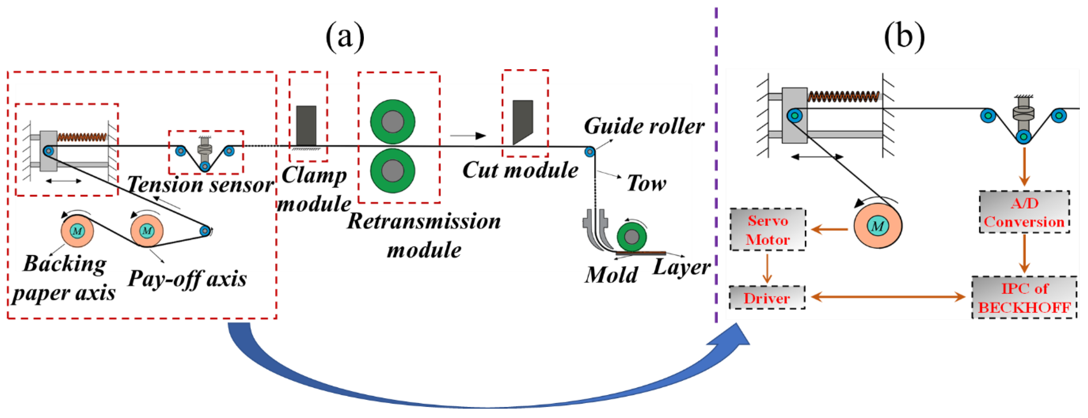
2. Model of the Tension Fluctuation for AFP

The range of tension fluctuations significantly impacts the stability and reliability of laying. Therefore, it is crucial to model the tension fluctuations during AFP. Considering the working conditions, several issues must be explored when modeling tension fluctuations. Firstly, the clamping module, the retransmission module, and the cut module will frequently work alternately during the laying process, which will cause frequent abrupt changes in tension. Secondly, the laying speed and tension frequently change when the large curvature mold is laid. Thus, to address the above problems, this paper established a tension fluctuation model in the laying process, which reflected the tension variation rule under different working conditions. The schematic diagram of the tension control system is shown in Figure 1b.

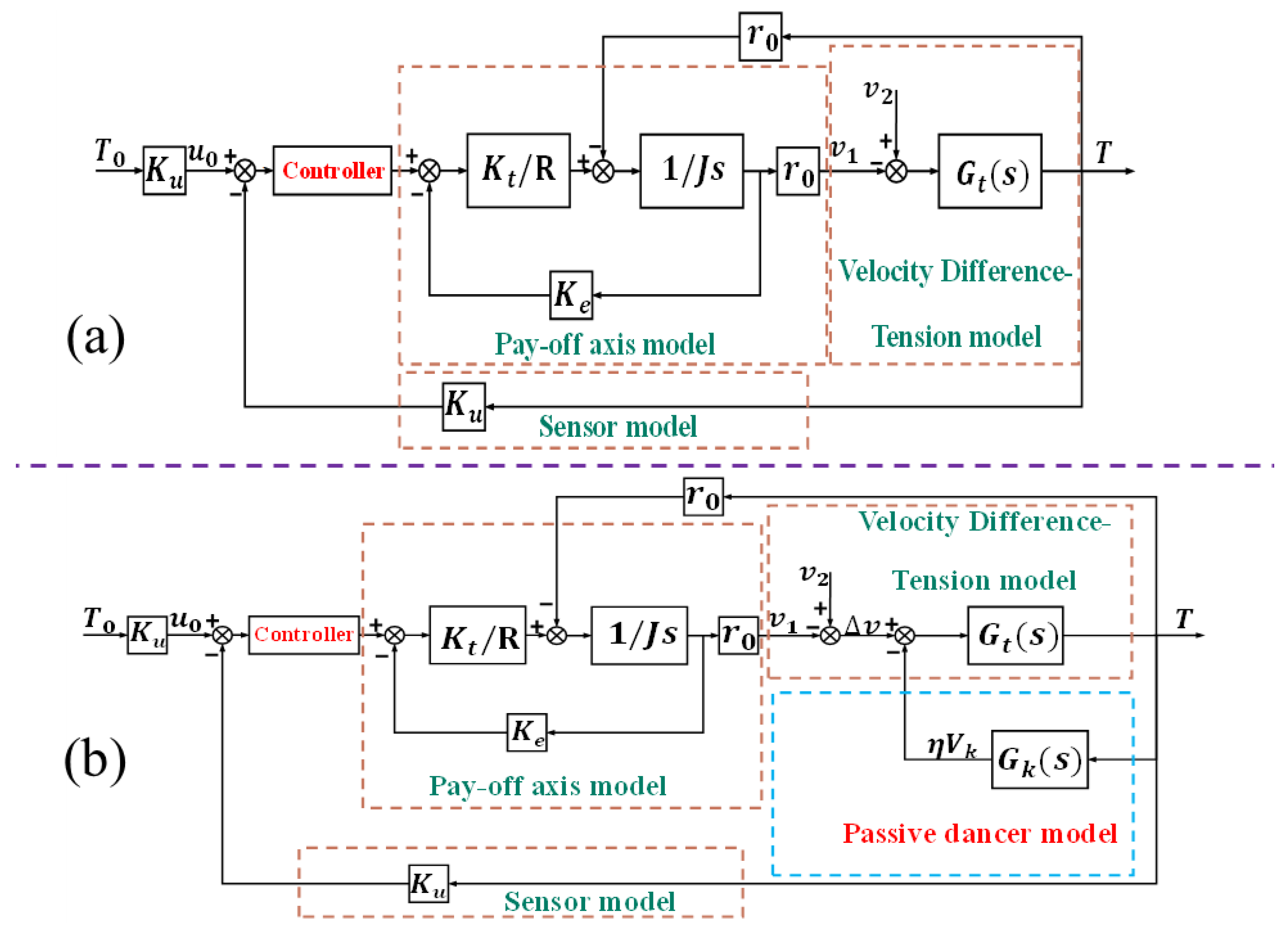
2.1. The Model for the Pay-off Axis

Figure 2a shows the schematic diagram of the pay-off axis working. The motor used for the pay-off axis was a permanent magnet synchronous servo motor (PMSM), which directly drove the pay-off axis. Therefore, the pay-off axis and servo motor were modeled as a whole in this paper. The space magnetic field distribution was sine, and the magnetic circuit’s core magnetic saturation and nonlinear characteristics were ignored. Thus, according to the torque balance equation, the equation of motion of the pay-off axis was obtained as follows:

$$M_t-T\left(t\right)r\left(t\right)+M_f=\dot{J}\left(t\right)\omega \left(t\right)+J\left(t\right)\dot{\omega }\left(t\right)+\beta \omega \left(t\right)$$

(1)

where $M_t$ is the resistance torque of motor output, $T\left(t\right)$ is the tow tension, $r\left(t\right)$ is the radius of the pay-off axis, $M_f$ is the dry friction torque, and $\beta$ is the viscous friction coefficient. $J\left(t\right)$ is the rotational inertia and $\omega \left(t\right)$ is the rotating angular velocity of the pay-off axis.

According to Equation (1), the equation of motion of the pay-off axis is strongly time-varying. Hence, to simplify the problem, the following simplification was considered for Equation (1):

(1) Since within the experimental scope of this study, the variation in the radius of the pay-off axis was not significant and the change in radius had a negligible impact on the model established in this study, the radius of the pay-off axis was considered a constant in this study;

(2) Based on the simplification assumption (1), the change in the rotational inertia could also be neglected;

(3) Due to the characteristics of the PMSM, the dry friction torque of the system was not considered.

Therefore, Equation (1) was simplified as follows:

$$M_t-T\left(t\right)r_0=J\dot{\omega }\left(t\right)+\beta \omega \left(t\right)$$

(2)

The PMSM operated in the torque mode. Hence, the current vector control was adopted, and the relationship between current and voltage was expressed as [27]:

$$\frac{di}{dt}=\frac{u\left(t\right)-Ri\left(t\right)-p{\psi }_f\omega \left(t\right)}{L}$$

(3)

where $i$ and $u$ are the current and voltage, respectively. $L$ is the inductance; $R$, $p$, and ${\psi }_f$ are the motor winding resistance, the number of motor poles, and rotor flux, respectively.

Meanwhile, based on the electromagnetic torque equation, the relationship between the current and output torque was expressed as follows [27]:

$$M_t=\frac{3}{2}pi{\psi }_f$$

(4)

The back-EMF coefficient and torque constant of the motor were defined as [27]:

$$\left\{\begin{array}{c}{K}_e=p{\psi }_f\\ K_t=\frac{3}{2}p{\psi }_f\end{array}\right.$$

(5)

where $K_e$ and $K_t$ are the back-EMF coefficient and torque constant in turn, respectively.

By joining Equation (2) to (5), the differential equation between the rotating angular velocity and the voltage was acquired:

$$LJ\ddot{\omega \left(t\right)}+\left(L\beta +RJ\right)\dot{\omega \left(t\right)}+\left(K_t{K}_e+R\beta \right)\omega \left(t\right)=K_{t}u\left(t\right)-L{r}_0\dot{T\left(t\right)}-R{r}_{0}T\left(t\right)$$

(6)

We considered the small inductance $L$ of the PMSM and $R\beta \ll K_t{K}_e$. Thus, $L$ and $R\beta$ were ignored in this paper. Equation (6) was simplified as follows:

$${\tau }_m\dot{\omega \left(t\right)}+\omega \left(t\right)=K_{m}u\left(t\right)-K_c{K}_m{r}_{0}T\left(t\right)$$

(7)

where ${\tau }_m=\frac{RJ}{K_t{K}_e}$, $K_c=\frac{R}{K_t}$, and $K_m=\frac{1}{K_e}$.

The Laplace transform was applied to both ends of Equation (7). Hence, the transfer function of the motor was obtained as follows:

$$G_m\left(s\right)=\frac{\omega \left(s\right)}{u\left(s\right)-K_c{r}_{0}T\left(s\right)}=\frac{K_m}{{\tau }_{m}s+1}$$

(8)

If the output of the system is velocity, Equation (8) can be written as:

$$G_m\left(s\right)=\frac{v\left(s\right)}{u\left(s\right)-K_c{r}_{0}T\left(s\right)}=\frac{K_m{r}_0}{{\tau }_{m}s+1}$$

(9)

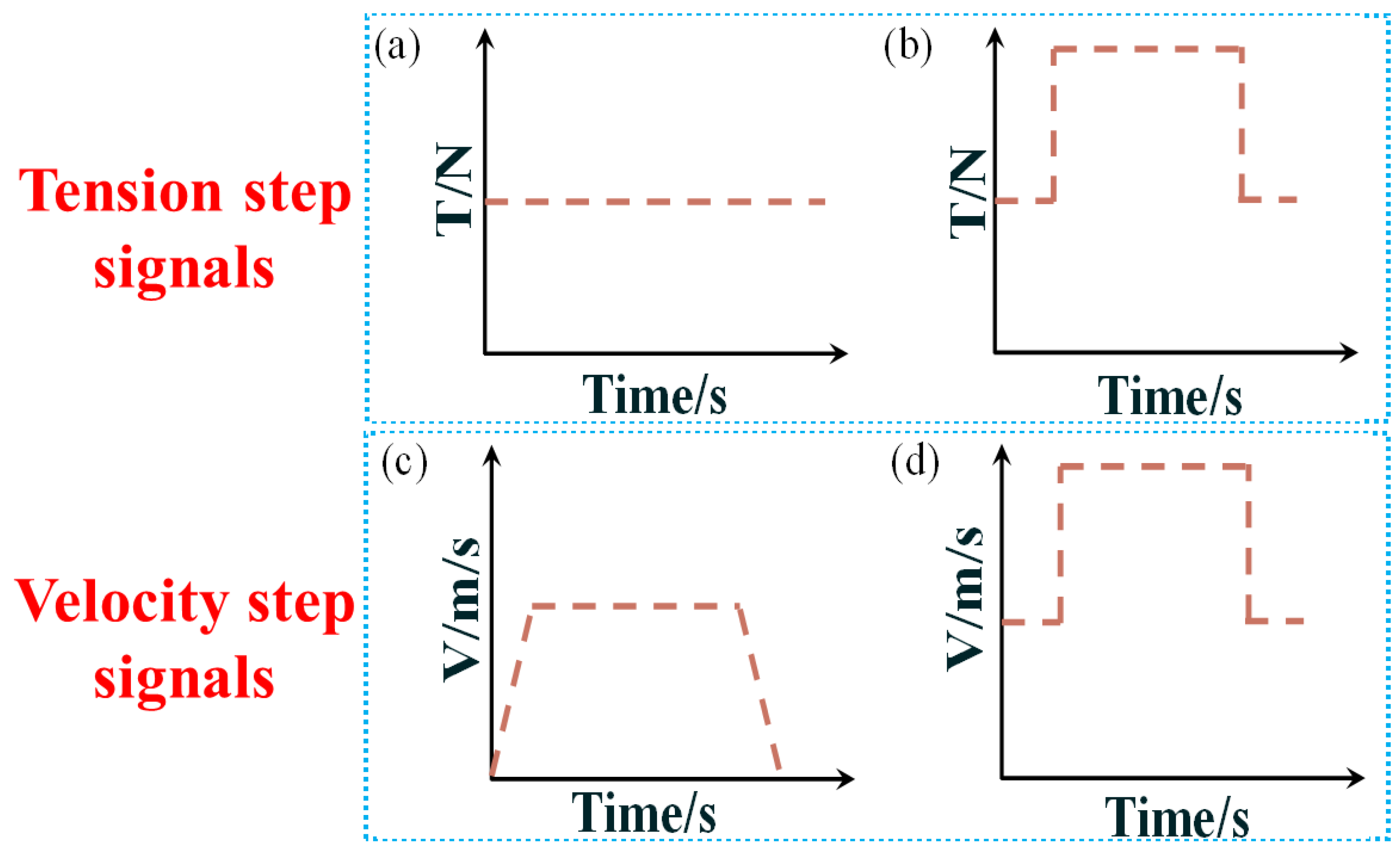
2.2. The Model for Velocity Difference–Tension

From the previous section, the speed of the pay-off axis will directly affect the tow tension. Meanwhile, for the AFP system, there is a strong coupling between the tow tension and the difference in speed. Therefore, the velocity difference–tension model is established in this section to achieve tension control.

To simplify the calculation, the AFP process shown in Figure 1a was simplified to the model shown in Figure 2b. In Figure 2b, index “1” means the tow is on the pay-off axis, “2” indicates that the tow is in the area where tension control is required, and “1-2” is the length of the laying area (the same below). In addition, the following laws need to be considered when establishing the velocity difference–tension model:

(1) Hooke’s law [28], which is used to define the elastic properties of the tow;

(2) The law of conservation of mass [29], which represents the cross-coupling between the velocity and tension of the tow;

(3) Newton’s laws of motion [30] described the dynamics of the passive dancers.

We considered that there was no mass transfer between the substances. Thus, by the law of conservation of mass, the following equation was obtained:

$$\frac{d}{dt}\left[{\int }_{x_1}^{x_2}\rho \left(x,t\right)A\left(x,t\right)dx\right]={\rho }_1{\left(x,t\right)A}_1\left(x,t\right)v_1\left(t\right)-{\rho }_2\left(x,t\right)A_2\left(x,t\right)v_2\left(t\right)$$

(10)

where $\rho$, $A$, and $v$ are the density, cross-sectional area, and velocity of the tow, respectively. $dx$ is the length of the tow in the unit area.

Since the tow is a transversely isotropic viscoelastic material [31], in the direction of motion, the tow is linearly elastic. The deformation of the tow can be obtained as follows:

$$d{x}_u=\left(1+\epsilon \right)d{x}_n$$

(11)

where $\epsilon$ is the tow strain. $u$ and $n$ are the tensioned and non-tensioned states of the tow, respectively.

Assuming the mass of the tow remains constant, then

$${\rho }_n{A}_{n}d{x}_n={\rho }_u{A}_{u}d{x}_u$$

(12)

Combining Equations (10)–(12) produces the following:

$$\frac{d}{dt}\left[{\int }_{x_1}^{x_2}\frac{{\rho }_u\left(x,t\right)A_u\left(x,t\right)dx}{1+{\epsilon }_2\left(x,t\right)}\right]=\frac{{\rho }_{1u}\left(x,t\right)A_{1u}\left(x,t\right)v_1\left(t\right)}{1+{\epsilon }_1\left(x,t\right)}-\frac{{\rho }_{2u}\left(x,t\right)A_{2u}\left(x,t\right)v_2\left(t\right)}{1+{\epsilon }_2\left(x,t\right)}$$

(13)

Considering the strain of the tow is equal everywhere in the control area, Equation (13) can be written as:

$$\frac{d}{dt}\left[{\int }_{x_1}^{x_2}\frac{1}{1+{\epsilon }_2\left(t\right)}\right]=\frac{v_1\left(t\right)}{1+{\epsilon }_1\left(t\right)}-\frac{v_2\left(t\right)}{1+{\epsilon }_2\left(t\right)}$$

(14)

During the tensile state, the tow strain on the pay-off axis is considered constant and much less than 1. From this, Equation (14) can be simplified to:

$$\frac{d}{dt}\left[\frac{L_0}{1+{\epsilon }_2\left(t\right)}\right]=\frac{v_1\left(t\right)}{1+{\epsilon }_0}-\frac{v_2\left(t\right)}{1+{\epsilon }_2\left(t\right)}\approx v_1\left(t\right)-\frac{v_2\left(t\right)}{1+{\epsilon }_2\left(t\right)}$$

(15)

where $L_0$ is the total length of the tow in the control area.

The simplification of Equation (15) produces:

$$-L_0\frac{d{\epsilon }_2\left(t\right)}{dt}={\left(1+{\epsilon }_2\left(t\right)\right)}^2{v}_1\left(t\right)-\left(1+{\epsilon }_2\left(t\right)\right)v_2\left(t\right)$$

(16)

According to the $\epsilon \ll 1$, we obtained:

$${\left(1+{\epsilon }_2\left(t\right)\right)}^2=1+2{\epsilon }_2\left(t\right)$$

(17)

The loss between the tow and each mechanism was ignored. Substituting Equation (17) into (16) and combined with Hooke’s law $\left(T\left(t\right)=EA{\epsilon }_2\left(t\right)\right)$, the following equation was obtained:

$$L\frac{dT\left(t\right)}{dt}=EA\left(v_2\left(t\right)-v_1\left(t\right)\right)+T\left(t\right)\left(v_2\left(t\right)-2v_1\left(t\right)\right)$$

(18)

where $E$ is the tow elastic modulus.

2.3. The Model of Passive Dancers

The schematic diagram of the passive dancers is shown in Figure 2c. We obtained from the geometric relationship that

$$L_1^{\prime }=L_1-\delta L_1=\frac{\sin {\theta }_1{L}_1-x\left(t\right)}{\sin \left({\theta }_1-\delta {\theta }_1\left(t\right)\right)}$$

(19)

where $x\left(t\right)$ and $\delta L_1$ are the passive dancer movement distance and upstream variation in the tow length, respectively.

Since $\delta {\theta }_1\left(t\right)$ is small during AFP, Equation (19) can be simplified as:

$$L_1^{\prime }=L_1-\frac{x\left(t\right)}{\sin {\theta }_1}$$

(20)

At the same time,

$$L_2^{\prime }=L_2-\frac{x\left(t\right)}{\sin {\theta }_2}$$

(21)

The passive dancer is subjected to tow tension, spring, and damping forces. Hence, the following equation is acquired by Newton’s second law of motion:

$$m\ddot{x\left(t\right)}=T\left(t\right)\left(\sin \left({\theta }_1-\delta {\theta }_1\left(t\right)\right)+\sin \left({\theta }_2-\delta {\theta }_2\left(t\right)\right)\right)-D\dot{x\left(t\right)}-Kx\left(t\right)$$

(22)

where $m$, $D$, and $K$ are the mass, damping, and elasticity coefficient of the passive dancer, respectively.

According to the geometric relationship shown in Figure 2c, it could also be obtained that:

$$\mathit{sin}\left({\theta }_1-\delta {\theta }_1\left(t\right)\right)=\frac{c_1-x\left(t\right)}{\sqrt{{\left(c_1-x\left(t\right)\right)}^2+h_1}}$$

(23)

From the above, it is evident that $x\left(t\right)$ is small. Thus, Equation (23) can be simplified and written as:

$$\frac{c_1-x\left(t\right)}{\sqrt{{\left(c_1-x\left(t\right)\right)}^2+{h_1}^2}}\approx \frac{c_1}{\sqrt{c_1^2+h_1^2}}$$

(24)

Similarly, it can be obtained that:

$$\sin \left({\theta }_2-\delta {\theta }_2\left(t\right)\right)\approx \frac{c_2}{\sqrt{c_2^2+h_2^2}}$$

(25)

where $c_2=c_2^{\prime }+x\left(t\right)$.

Let $q_1=\frac{c_1}{\sqrt{c_1^2+h_1^2}}, q_2=\frac{c_2}{\sqrt{c_2^2+h_2^2}}$, so that Equation (22) can be expressed as:

$$m\ddot{x\left(t\right)}=T\left(t\right)\left(q_1+q_2\right)-D\dot{x\left(t\right)}-Kx\left(t\right)$$

(26)

The Laplace transform was applied to both ends of Equation (26). Therefore, the transfer function of passive dancers could be written as follows:

$$G_k\left(s\right)=\frac{x\left(s\right)}{T\left(s\right)}=\frac{\left(q_1+q_2\right)}{m{s}^2+Ds+K}$$

(27)

2.4. The Model of the Tension Control with Passive Dancers

During AFP, passive dancers are in the left and right movements. Combining Equations (20) and (21), the total length of the tow can be defined as follows:

$$L^{\prime }=L_0-\delta L_1-\delta L_2=L-\left(\frac{1}{\sin {\theta }_1}+\frac{1}{\sin {\theta }_2}\right)x\left(t\right)$$

(28)

Let $\frac{1}{\sin {\theta }_1}+\frac{1}{\sin {\theta }_2}=\eta .$ Taking Equation (28) into (15), the following equation can be obtained:

$$\frac{d}{dt}\left[\frac{L_0-\eta x\left(t\right)}{1+{\epsilon }_2\left(t\right)}\right]=\frac{v_1\left(t\right)}{1+\epsilon }-\frac{v_2\left(t\right)}{1+{\epsilon }_2\left(t\right)}\approx v_1\left(t\right)-\frac{v_2\left(t\right)}{1+{\epsilon }_2\left(t\right)}$$

(29)

In addition, Equation (27) can be written as:

$$G_k\left(s\right)=\frac{\eta V_k\left(s\right)}{T\left(s\right)}=\frac{\eta \left(q_1+q_2\right)s}{m{s}^2+Ds+K}$$

(30)

Similar to Equation (18), using Hooke’s law, it can be obtained as follows:

$$\left(L_0-\eta x\left(t\right)\right)\frac{dT\left(t\right)}{dt}=EA\left(v_2\left(t\right)-v_1\left(t\right)-\eta \frac{dx}{dt}\right)+T\left(t\right)\left(v_2\left(t\right)-2v_1\left(t\right)-\eta \frac{dx}{dt}\right)$$

(31)

Linearizing Equation (31), let $V_n=v_n-v_{nr}, T_l=T-t_r, and X=x-x_r$. Substituting $V_n$, $T_l$, and $X$ into Equation (31), the linearized tensorial dynamics can be derived as:

$$\left(L_0-\eta x_r\right)\frac{d{T}_l}{dt}=\left(EA+t_r\right)\left(V_2-V_1-\eta \frac{dX}{dt}\right)+T_l\left(v_{2r}-2v_{1r}\right)-V_1{t}_r$$

(32)

Defining $L_0-\eta x_r=\gamma$ and applying the Laplace transform to Equation (32) produces:

$$\left(\gamma s-v_{2r}+2v_{1r}\right)T_l\left(s\right)=\left(EA+t_r\right)V_2\left(s\right)-\left(EA+{2t}_r\right)V_1\left(s\right)-\eta \left(EA+t_r\right)sX\left(s\right)$$

(33)

Since $EA\gg t_r$, so

$$EA+{2t}_r\approx EA+t_r$$

(34)

Substituting Equation (34) into Equation (33), the following transfer function is derived

$$G_t\left(s\right)=\frac{T_l\left(s\right)}{V_2\left(s\right)-V_1\left(s\right)-\eta V_k\left(s\right)}=\frac{EA+t_r}{\gamma s-v_{2r}+2v_{1r}}$$

(35)

The tension sensor can be treated as an amplifier link due to the short delay. Therefore, the transfer function of the sensor is

$$G_{sen}\left(s\right)=K_u$$

(36)

When tension is controlled during AFP, nonlinear and time-variant problems are insignificant. Hence, the integral separated PID was chosen as the system’s control strategy. The control law is shown below:

$$\lambda =\left\{\begin{array}{c}1, \left|e\left(k\right)\right|\le e_0\\ 0, \left|e\left(k\right)\right|>e_0\end{array}\right.$$

(37)

$$u\left(t\right)=K_{P}e\left(t\right)+\lambda K_I\sum _{j=0}^{k}e\left(j\right)T_t+K_D\frac{e\left(k\right)-e\left(k-1\right)}{T_t}$$

(38)

where $u\left(t\right)$ is the controlled voltage. $T_t$, $\lambda$, and $e_0$ is the sampling time, control coefficient of integral terms, and set threshold, respectively.

Combining Equations (9), (27), (35), (36) and (38), the control framework of the system can be obtained, as shown in Figure 3b. If the passive dancer is disregarded in this system, the control diagram is as shown in Figure 3a.

The transfer function derivation method of the system that neglects the passive rollers is similar to the above. Thus, this paper’s derivation of this transfer function was not carried out. The system equations are as follows:

$$G_t\left(s\right)=\frac{T_l\left(s\right)}{V_2\left(s\right)-V_1\left(s\right)}=\frac{EA+t_r}{L_{0}s-v_{2r}+2v_{1r}}$$

(39)

3. Analysis of the Precise Tension Control Model

In this section, Simulink simulates the spring damping and elasticity coefficient effects on the tension fluctuations at different stages of the AFP. The passive dancer parameters that make the system perform better were selected by analyzing the results. The specific simulated stages were clamping, retransmission, and laying. This paper simplified these processes as tension step signals, velocity perturbations, and the combination of tension step and velocity step, respectively. The required parameters for the simulation are shown in

Table 1. The required parameters for the simulation.

Parameters	Value	Parameters	Value
$K_t$	0.8 Nm/A	$K_u$	0.5 mv/N
$K_e$	58 V/Krpm	$E$	52.33 GPa
$R$	$11.3 \mathsf{\Omega }$	$A$	$7.94\times {10}^{-7} {\mathrm{m}\mathrm{m}}^2$
$J$	$0.00018 \mathrm{K}\mathrm{g}·{\mathrm{m}}^2$	$L$	1 m
$r_0$	0.075 m	$v_{1r}$	60 mm/s
$K_p$	5	$v_{2r}$	60 mm/s, 30 mm/s
$K_I$	200	$t_r$	5 N
$K_D$	0.1	$x_r$	0.1 m
$m$	0.3 kg	${\theta }_1, {\theta }_2$	${75.9}^{°}, {81.2}^{°}$
$h_1$	0.081 m	$h_2$	0.034 m
$c_1$	0.312 m	$c_2$	0.268 m

, and the step function is illustrated in Figure 4.

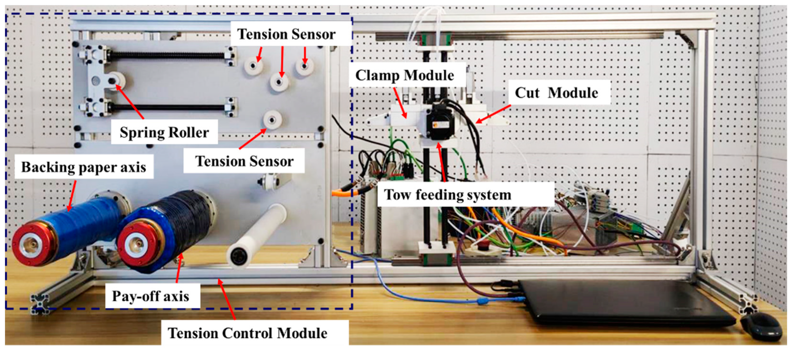
3.1. Model Validation

Figure 5 shows the experimental platform of the automatic wire-feeding used to carry out the experiments for verifying the model’s validity. The tow used for experiments was a unidirectional carbon/epoxy tow with a width of 6.35 mm (Type: USN12500/7901). The parameters of the tow are shown in Table 1. In Figure 5, the experimental platform is equipped with two rotating axes, the pay-off axis and the backing paper axis, driven by torque servo motors. The pay-off axis holds the filament roll, while the backing paper axis holds the backing paper roll. The filament roll is the source of tows. As the filament pay-off axis rotates, the tows within the filament roll unwind, allowing the tows to enter the filament bundle conveying mechanism. Meanwhile, the backing paper that wraps around the tows separates from the tows and is collected back onto the backing paper roll. After leaving the filament roll, the tows pass through the guide roller, several guide wheels, and tension sensing device and smoothly enter the filament bundle action mechanism. The bundle action mechanism consists of a clamp module, a tow feeding system, and a cut module. The clamping module is responsible for fixing the position of the tow when the feeding system is not operational. The feeding system is accountable for transporting the tow forward, while the cut module is responsible for cutting the tow.

The operating principle of the experimental platform shown in Figure 5 is as follows: The unwound tows from the filament roll smoothly enter the spring roller mechanism through the reversing device. The spring roller consists of a guide wheel, a translating guide rail, and a spring. The tension of the tows drives the guide wheel to move along the guide rail until a state of force equilibrium is achieved. The tension-sensing device can convert tension into pressure on the guide wheel, indirectly measuring the tension of the bundles. The clamping module is driven by a cylinder, where the extension and retraction of the cylinder’s piston rod drive the closure of the clamping block, thereby achieving the function of fixing the tow. The tow feeding system consists of a pair of mutually movable rollers, with the lower roller driven by a motor, rotating in real-time. The tows are positioned between the two rollers. When the upper roller clamps the tows between the rollers under the action of the cylinder, the tows are driven forward by the frictional force of the rollers, following the linear velocity of the rollers. The cut module is propelled by a cylinder to cut the tows using the cutting blade.

The IPC, motor, and sensor models used in this experiment platform were C6130, AKM33E, and FS127, respectively. Furthermore, the system was designed as a function block and utilized the EtherCAT Fieldbus protocol for communication.

The tension control flow chart is shown in Figure 6. It can be obtained from the flow chart that the system essentially controls the tension by controlling the motor torque. Thus, the motor torque needs to be calibrated before the experiment, and the calibration result is:

$$y_{torque}=0.0059x-0.011$$

(40)

where $x$ is the digital output of the PLC and $y_{torque}$ is the actual output torque of the motor. Equation (40) calculates the torque in the flow chart.

The pressure, target tension, and retransmission speed were set as 0.6 MPa, 5 N, and 60 mm/s, respectively. The relative humidity was 65%, and the ambient temperature was 25 °C. Based on the automatic wire-feeding experimental platform established in Figure 5, the following three experiments were carried out to verify the validity of the tension system model established in this paper:

(1) The tow was clamped in the stationary state, after which a tension step of 5 N was applied. This process is depicted in Figure 7a. It can also be observed from Figure 7a that the actual tension values overlap very well with the simulated values.

(2) The lower roller of the feeding module was set to 60 mm/s. At the moment of feeding module initiation, the upper roller was pressed down, and the clamping block was lifted, causing the tow to be driven forward by the friction of the roller. Due to the tow’s significant friction and low mass, it rapidly accelerated from zero to 60 mm/s with a very high acceleration. Therefore, the moment of feeding module initiation can be considered as a velocity step process. After a brief yet significant disturbance, the tension quickly stabilized and fluctuated within a small range near 5 N. After maintaining a steady delivery speed of 60 mm/s for a while, the lower roller speed was reduced to 0, resulting in another significant fluctuation in tension. However, the tension quickly returned to 5 N. Figure 7b records the tension fluctuations throughout this process. The experimental curve shows a high degree of agreement with the simulated curve. In particular, as revealed in Figure 7b, small tension fluctuations occur during wire feeding, which is unavoidable and acceptable.

(3) The tow feeding speed was set as a sine wave. For the tension system, the tension value is outputted as a sinusoidal wave with the same frequency, as shown in Figure 7c. It can also be observed from Figure 7c that the tension amplitude and the phase difference with the speed signal exhibit a high degree of agreement between the experimental and simulated results.

In conclusion, the tension system model established in this study has a high credibility.

3.2. Analysis of the System Stability and Superiority

In classical control theory, the dynamic performance of a model is typically described using step response, and the most important parameters in the step response are the maximum overshoot ($M_p$), rise time ($T_r$), and settling time ($T_s$). Therefore, in this study, we considered using these three parameters to assess the quality of the established tension system. Specific analyses are provided below.

Before performing the simulation, it is necessary to determine the stability and superiority of the model with the passive dancer developed in this paper. Figure 8 shows the Bode diagram of the system (without a controller) with different damping and elasticity coefficients. In Figure 8a, both $G_m$ (gain margin) and $P_m$ (phase margin) are infinite, which indicates that the established model is steady. Moreover, the larger the $D$, the wider the medium frequency, and the smoother the system in the medium frequency. Meanwhile, in the high band, the system decays faster with a larger $D$, which demonstrates the ability of the system to resist high-frequency interference. The pattern in Figure 8b is similar to that in Figure 8a. Thus, Figure 8b was not analyzed in this paper.

As shown in Figure 9, the tension fluctuations under clamping, retransmission, and laying processes were analyzed, respectively. In Figure 9, compared to the other two systems, the system without passive dancers has a larger $M_p$ and a shorter $T_r$ and $T_s$. However, for the tension control system in AFP, if the $T_r$ and $T_s$ are excessively short, the motor does not have enough time to respond, and the tension varies rapidly. In this case, the probability of laying defects increases. Meanwhile, for the system without the controller, all indicators are inferior to those with a passive roller and controller. In contrast to the other two systems, the tension control system with the passive dancers and the controller provides a better buffer for the motor and reduces the maximum overshoot significantly, which is better for the AFP.

3.3. Selection of the Passive Dancer Parameters during Different Stages

For AFP, the tension control system needs an excellent buffering mechanism, small tension fluctuations, and faster stabilization. In other words, the smaller the $T_r$, $M_p$, and $T_s$, the better the system performance. But in practice, perfect systems are almost non-existent. This paper proposed a new evaluative method to evaluate the performance of the established tension control system and selected the appropriate passive dancer parameters. The principle of this method is as follows: Firstly, a total score is defined for a perfect system. Secondly, the defined total score is assigned according to the different importance of each performance indicator ($M_p$, $T_s$, and $T_r$) to the system, and then the value of each performance indicator is multiplied by its assigned score. Finally, the resulting values are added to obtain a value, and the magnitude of this value evaluates the system. In this paper, a total score of 10 was defined. And by analyzing the AFP, $M_p$, $T_s$, and $T_r$ were defined to be 5, 3, and 2 scores, respectively. It should be noted that allocating 10 points in a 5-3-2 ratio is more of a demonstration and an example. While this specific allocation of 5-3-2 may not be perfect, it reflects the requirements of a certain type of layup process. These requirements can be dynamically adjusted based on the actual needs of the process personnel. The calculation formula for evaluating the tension control system is as follows:

$$\delta =\frac{{5V}_{M_p}}{100}+3V_{T_s}+{2V}_{T_r}$$

(41)

where $\delta$ is the system score, which is used to judge the system performance. $V_{M_p}$, $V_{T_s}$, and $V_{T_r}$ are the values of $M_p$, $T_s$, and $T_r$ for different systems, respectively. As for AFP, the smaller the $\delta$, the better the system performance.

This section analyzes the effect of different damping and elasticity coefficients on the system during different working stages in AFP.

The tension step signal mainly causes tension fluctuation during the clamping stage, and the result is shown in Figure 10. Figure 10a,b show the tension fluctuations and performance analysis of the control system under different damping conditions, respectively. From Figure 10a, it can be seen that, as $D$ increases, $T_s$ and $T_r$ decrease gradually. This is due to the fact that the greater the $D$, the lower the passive dancer deformation, and the better the ability to absorb shock and buffer. Therefore, less time is required for the system to stabilize. In particular, when $D$ increases from $5 \mathrm{N}·\mathrm{s}/\mathrm{m}$ to $100 \mathrm{N}·\mathrm{s}/\mathrm{m}$, $M_p$ progressively decreases. However, as $D>100 \mathrm{N}·\mathrm{s}/\mathrm{m}$, $M_p$ starts to rise gradually. This is because $D$ is excessively large, and the passive dancer moves very slowly. Thus, to make the system reach stability faster, $M_p$ becomes greater. In addition, combining Figure 10a,b, it could be obtained that, when $D=5 \mathrm{N}·\mathrm{s}/\mathrm{m}$, $50 \mathrm{N}·\mathrm{s}/\mathrm{m}$, and $100 \mathrm{N}·\mathrm{s}/\mathrm{m}$, the system performance is poor. However, the system performs well when $D=200 \mathrm{N}·\mathrm{s}/\mathrm{m}$ and $400 \mathrm{N}·\mathrm{s}/\mathrm{m}$. Therefore, both $D=200 \mathrm{N}·\mathrm{s}/\mathrm{m}$ and $400 \mathrm{N}·\mathrm{s}/\mathrm{m}$ can be considered as the damping coefficients for the clamping stage.

In the clamping phase, the elasticity coefficient also impacts the control system performance, and the results are shown in Figure 10c,d. As $K$ increases, the distance traveled by the passive rollers and the response time of the system decrease, but the force required to reach equilibrium increases. Hence, as shown in Figure 10a, when $K$ increases, $M_p$ progressively increases, while $T_r$ and $T_s$ diminish. Furthermore, combining Figure 10c,d, it could be concluded that, compared to $K=100 \mathrm{N}/\mathrm{m}$ and $300 \mathrm{N}/\mathrm{m}$, the system performance is better when $K=600 \mathrm{N}/\mathrm{m}$,$900 \mathrm{N}/\mathrm{m}$, and $1800 \mathrm{N}/\mathrm{m}$. Therefore, the elasticity factor of the clamping stage was chosen as $K=600 \mathrm{N}/\mathrm{m}$, $900 \mathrm{N}/\mathrm{m},$ and $1800 \mathrm{N}/\mathrm{m}$. In particular, the damping coefficient has a more significant effect on the system than the elasticity coefficient, as shown in Figure 10.

During the retransmission phase of the AFP, the tow suddenly accelerates or decelerates at the beginning and end of the transmission. Thus, in this study, the cause of tension fluctuation in the retransmission stage was simplified to a speed step. The effect of different passive dancer parameters on tension fluctuation during the retransmission stage was analyzed, and the results are shown in Figure 11. It should be noted that the tow had already an applied tension of 5 N at the beginning of the retransmission period. Hence, when analyzing the tension control system in the retransmission phase, $T_r$ was not considered. Comparing Figure 11 and Figure 10, all the performance indicators of the tension system become more significant with the velocity step, which indicates that the velocity step has a greater effect on tension fluctuations than the tension step.

Figure 11a,b show the effect of different damping coefficients on the tension fluctuation during the retransfer process. From Figure 11a, it can be concluded that, as $D$ increases, $T_s$ gradually decreases, while $M_p$ first reduces and then rises, which is similar to what occurs during the clamping stage. In particular, compared to the clamping phase, the damping value that makes $M_p$ change from a downward to an upward trend is greater in the retransmission phase. This is because the speed step has more influence on the tension fluctuation than the tension step. Therefore, more damping force must be provided for buffering to reduce the tension swing during retransmission. In addition, combining Figure 8a,b, it also can be obtained that the system has a low resistance to tension fluctuation when $D=5 \mathrm{N}·\mathrm{s}/\mathrm{m}$ and $50 \mathrm{N}·\mathrm{s}/\mathrm{m}$. And when $D=100 \mathrm{N}·\mathrm{s}/\mathrm{m}$, $200 \mathrm{N}·\mathrm{s}/\mathrm{m}$, and $400 \mathrm{N}·\mathrm{s}/\mathrm{m}$, the overall performance of the system is better. Therefore, $D=100 \mathrm{N}·\mathrm{s}/\mathrm{m}$, $200 \mathrm{N}·\mathrm{s}/\mathrm{m}$, and $400 \mathrm{N}·\mathrm{s}/\mathrm{m}$ were all considered as the damping values for the retransmission phase.

Figure 11c,d show the control system’s tension fluctuations and performance analysis for the retransmission phase with different elasticity coefficients, respectively. Similar to what occurs during the clamping stage, $M_p$ gradually increases with the increase in $K$, while $T_s$ decreases. However, in the retransmission stage, the change in performance indicator parameters is insignificant with the K change, which indicates that the K variation could not greatly suppress the tension fluctuation during the retransmission stage. Meanwhile, by analyzing Figure 11c,d, $K=600 \mathrm{N}/\mathrm{m}$, $900 \mathrm{N}/\mathrm{m}$, and $1800 \mathrm{N}/\mathrm{m}$ were all considered as the elasticity coefficients of the retransmission phase.

Since the tension fluctuation law in the layup phase is similar to that in the retransmission stage, the only difference is that, compared to the retransmission phase, the tension fluctuation in the layup phase is much larger. This difference is because the tension in the layup stage suffers from tension step and velocity step effects. Thus, the discussion of tension fluctuations in the layup stage was not carried out in this paper. Only the corresponding conclusions are provided: The values of $100 \mathrm{N}·\mathrm{s}/\mathrm{m}$, $200 \mathrm{N}·\mathrm{s}/\mathrm{m}$, and $400 \mathrm{N}·\mathrm{s}/\mathrm{m}$ were considered as the damping coefficients in the layup phase. Meanwhile, 600 N/m, 900 N/m, and 1800 N/m were selected as the elasticity coefficients.

The above analysis shows that the passive dancer parameters significantly affect the tension fluctuations during the clamping, retransmission, and layup processes. At the same time, compared to the retransmission and layup stages, the clamping process does not require a high system performance, especially $T_s$. In summary, this section considered the damping and elasticity coefficients determined during the retransmission and layup phases as the passive dancer parameters for the AFP process.

3.4. Layup Experiments

Placement experiments were carried out using the passive dancer parameters selected by the simulation. The test setup is shown in Figure 12a. This study focused solely on investigating the influence of tension on the layup process. In this experiment, only tension was treated as a variable, while the remaining parameters were kept constant. Therefore, we assumed that any observed effects were attributed to the tension system itself rather than changes in other parameters. The experimental results show fewer layup defects are generated when the selected parameters are used for a layup, and the quality is high. As depicted in Figure 12b, the tension fluctuates excessively when D = 400 N/(m/s). Thus, it is easier to obtain pucker and edge unevenness during laying. As for D = 100 N/(m/s) and 200 N/(m/s), there is a missing tow in the laying process, which could be ignored. It can be seen from Figure 12c that the variation in the elasticity coefficient does not have much effect on the layup. When K = 600 N/m, sticking occurs during laying. And when K = 900 N/m and K = 1800 N/m, there are small wrinkles during laying. Since defects are unavoidable, the minor defects caused by changing the elasticity coefficient during the laying process were neglected. In addition, comparing the influence of the damping coefficient and elasticity coefficient on the laying process, it could be obtained that the damping coefficient has a more significant effect. (Note: The results are only for the type of prepreg selected in this paper, the AFP parameters, and the mold used for a layup. If the above conditions change, the simulation and experiments must be reconducted to determine the passive dancer parameters).

4. Conclusions

This paper establishes a precise tension fluctuation model to describe the pattern of tension variation during AFP. The tests confirm the effectiveness of this model, and the Bode diagram illustrates the system’s stability. Moreover, the superiority of the tension control system with passive rollers is demonstrated by simulation analysis. After that, the tension fluctuations under different elasticity coefficients and damping are obtained for each phase in the AFP. The evaluation method developed in this article determines the passive dancer parameters with a better system performance. Furthermore, placement experiments are carried out using the determined passive dancer parameters.

(1)

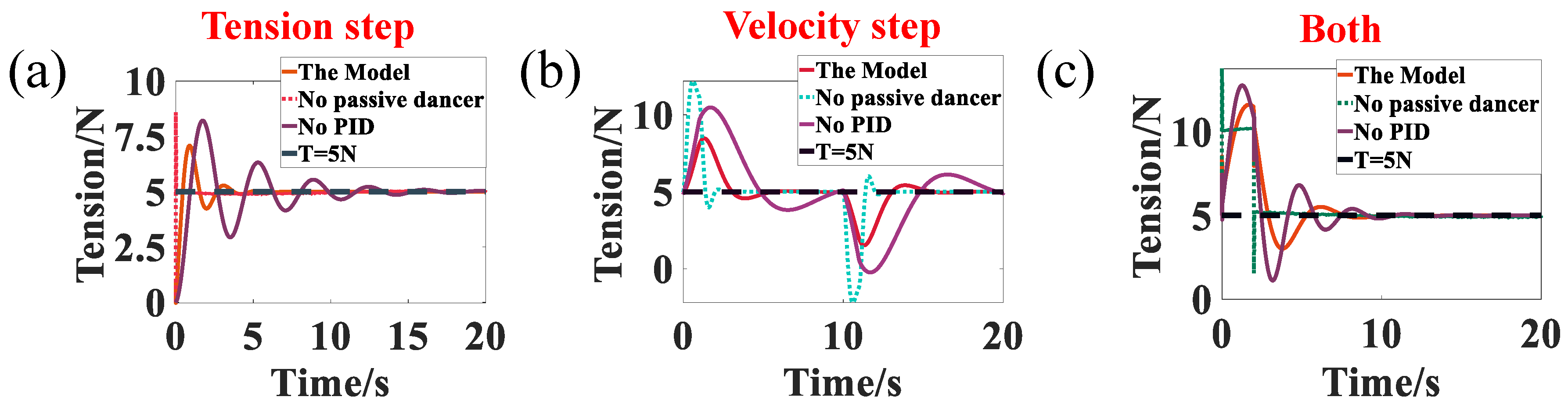
The model’s validity was verified by developing wire-feeding and clamping experiments. Also, the stability and superiority of the control system with a passive dancer were illustrated by simulation analysis. The system provides a better buffer for the motor and reduces the maximum overshoot significantly.

(2)

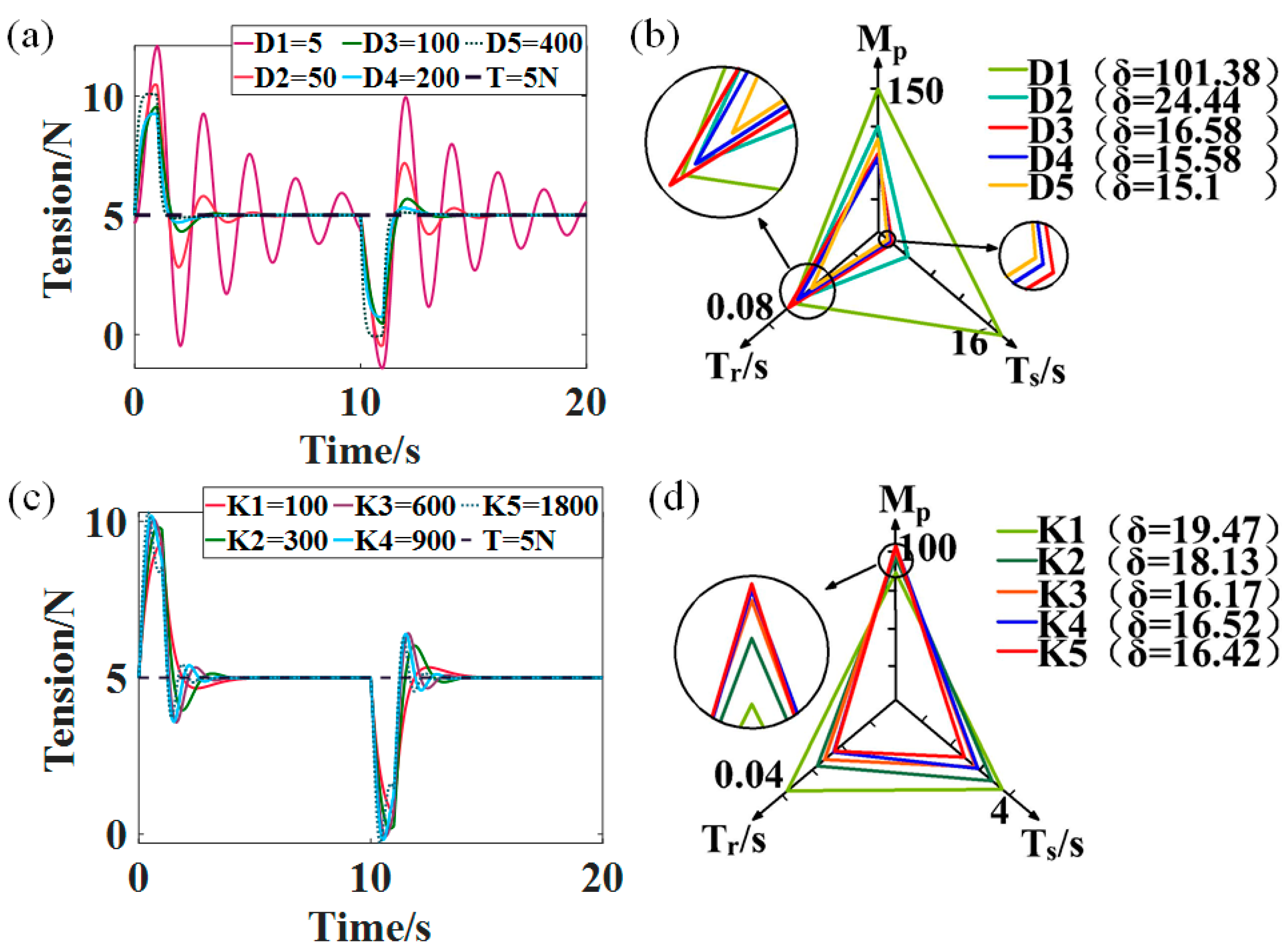
The tension fluctuation at each stage of AFP can be derived from the precise tension control model. By analyzing the tension fluctuation with different passive dancer parameters, it can be concluded that the damping has more influence on the tension fluctuation than the elasticity coefficient. Meanwhile, by appropriately increasing the damping and elasticity coefficients, the system performance is improved, and the tension fluctuation is reduced, thus enhancing the layup quality.

(3)

By analyzing the tension fluctuations at each stage, the elastic coefficients of the passive dancer in the AFP process were determined to be 600 N/m, 900 N/m, and 1800 N/m, and the damping was 100 N∙s/m, 200 N∙s/m, and 400 N∙s/m. Furthermore, it was demonstrated that using the determined passive dancer parameters for laying could improve the laying quality significantly.

References

1. Kumar, S.; Prasad, L.; Patel, V.K.; Kumar, V.; Kumar, A.; Yadav, A.; Winczek, J. Physical and Mechanical Properties of Natural Leaf Fiber-Reinforced Epoxy Polyester Composites. Polymers 2021, 13, 1369. [Google Scholar] [CrossRef]
2. Alonso-Montemayor, F.J.; Tarrés, Q.; Oliver-Ortega, H.; Espinach, F.X.; Narro-Céspedes, R.I.; Castañeda-Facio, A.O.; Delgado-Aguilar, M. Enhancing the Mechanical Performance of Bleached Hemp Fibers Reinforced Polyamide 6 Composites: A Competitive Alternative to Commodity Composites. Polymers 2020, 12, 1041. [Google Scholar] [CrossRef] [PubMed]
3. Katouzian, M.; Vlase, S. Creep Response of Carbon-Fiber-Reinforced Composite Using Homogenization Method. Polymers 2021, 13, 867. [Google Scholar] [CrossRef] [PubMed]
4. Wang, B.; He, B.; Wang, Z.; Qi, S.; Zhang, D.; Tian, G.; Wu, D. Enhanced Impact Properties of Hybrid Composites Reinforced by Carbon Fiber and Polyimide Fiber. Polymers 2021, 13, 2599. [Google Scholar] [CrossRef]
5. Liu, F.; Zhang, W.; Shang, J.; Yi, M.; Wang, S.; Ding, X. A Planar Underactuated Compaction Mechanism with Self-Adaptability for Automated Fiber Placement Heads. Aerospace 2022, 9, 586. [Google Scholar] [CrossRef]
6. Schmidt, C.; Schultz, C.; Weber, P.; Denkena, B. Evaluation of Eddy Current Testing for Quality Assurance and Process Monitoring of Automated Fiber Placement. Compos. Part B Eng. 2014, 56, 109–116. [Google Scholar] [CrossRef]
7. Alshahrani, H.; Hojjati, M. A Theoretical Model with Experimental Verification for Bending Stiffness of Thermosetting Prepreg During Forming Process. Compos. Struct. 2017, 166, 136–145. [Google Scholar] [CrossRef]
8. Smith, A.W.; Endruweit, A.; Choong, G.Y.H.; De Focatiis, D.S.A.; Hubert, P. Adaptation of Material Deposition Parameters to Account for Out-Time Effects on Prepreg Tack. Compos. Part A Appl. Sci. Manuf. 2020, 133, 105835. [Google Scholar] [CrossRef]
9. Bakhshi, N.; Hojjati, M. An Experimental and Simulative Study on the Defects Appeared During Tow Steering in Automated Fiber Placement. Compos. Part A Appl. Sci. Manuf. 2018, 113, 122–131. [Google Scholar] [CrossRef]
10. Bakhshi, N.; Hojjati, M. Effect of Compaction Roller on Layup Quality and Defects Formation in Automated Fiber Placement. J. Reinf. Plast. Comp. 2020, 39, 3–20. [Google Scholar] [CrossRef]
11. Lukaszewicz, D.H.J.A.; Ward, C.; Potter, K.D. The Engineering Aspects of Automated Prepreg Layup: History, Present and Future. Compos. Part B Eng. 2012, 43, 997–1009. [Google Scholar] [CrossRef]
12. He, R.; Qu, W.; Ke, Y. An Improved Path Discretization Method for Automated Fiber Placement. J. Reinf. Plast. Comp. 2020, 39, 545–559. [Google Scholar] [CrossRef]
13. Qu, W.; Pan, H.; Yang, D.; Li, J.; Ke, Y. As-Built Fe Thermal Analysis for Complex Curved Structures in Automated Fiber Placement. Simul. Model. Pract. Theory 2022, 118, 102561. [Google Scholar] [CrossRef]
14. Wu, J.; Cheng, L.; Guo, Y.; Li, J.; Ke, Y. Dynamic Modeling and Parameter Identification for a Gantry-Type Automated Fiber Placement Machine. CIRP J. Manuf. Sci. Technol. 2022, 37, 388–400. [Google Scholar] [CrossRef]
15. Qureshi, Z.; Swait, T.; Scaife, R.; El-Dessouky, H.M. In Situ Consolidation of Thermoplastic Prepreg Tape Using Automated Tape Placement Technology: Potential and Possibilities. Compos. Part B Eng. 2014, 66, 255–267. [Google Scholar] [CrossRef]
16. Liu, Y.; Fang, Q.; Ke, Y. Modeling of Tension Control System with Passive Dancer Roll for Automated Fiber Placement. Math. Probl. Eng. 2020, 2020, 9839341. [Google Scholar] [CrossRef]
17. Khan, M.A.; Mitschang, P.; Schledjewski, R. Parametric Study on Processing Parameters and Resulting Part Quality through Thermoplastic Tape Placement Process. J. Compos. Mater. 2013, 47, 485–499. [Google Scholar] [CrossRef]
18. He, Y.; Jiang, J.; Qu, W.; Ke, Y. Compaction Pressure Distribution and Pressure Uniformity of Segmented Rollers for Automated Fiber Placement. J. Reinf. Plast. Comp. 2022, 41, 427–443. [Google Scholar] [CrossRef]
19. Belhaj, M.; Dodangeh, A.; Hojjati, M. Experimental Investigation of Prepreg Tackiness in Automated Fiber Placement. Compos. Struct. 2021, 262, 113602. [Google Scholar] [CrossRef]
20. Pei, J.; Wang, X.; Pei, J.; Yang, Y. Path Planning Based on Ply Orientation Information for Automatic Fiber Placement On Mesh Surface. Appl. Compos. Mater. 2018, 25, 1477–1490. [Google Scholar] [CrossRef]
21. Zhao, C.; Xiao, J.; Wang, X. Effects of tows tension on automated fiber placement process. Acta Aeronaut. Astronaut. Sin. 2016, 37, 1384–1392. [Google Scholar]
22. Jiang, J.; He, Y.; Wang, H.; Ke, Y. Modeling and Experimental Validation of Compaction Pressure Distribution for Automated Fiber Placement. Compos. Struct. 2021, 256, 113101. [Google Scholar] [CrossRef]
23. Budelmann, D.; Detampel, H.; Schmidt, C.; Meiners, D. Interaction of Process Parameters and Material Properties with Regard to Prepreg Tack in Automated Lay-Up and Draping Processes. Compos. Part A Appl. Sci. Manuf. 2019, 117, 308–316. [Google Scholar] [CrossRef]
24. Qu, W.; He, R.; Cheng, L.; Yang, D.; Gao, J.; Wang, H.; Yang, Q.; Ke, Y. Placement Suitability Analysis of Automated Fiber Placement on Curved Surfaces Considering the Influence of Prepreg Tow, Roller and Afp Machine. Compos. Struct. 2021, 262, 113608. [Google Scholar] [CrossRef]
25. Hirsch, P.; John, M.; Leipold, D.; Henkel, A.; Gipser, S.; Schlimper, R.; Zscheyge, M. Numerical Simulation and Experimental Validation of Hybrid Injection Molded Short and Continuous Fiber-Reinforced Thermoplastic Composites. Polymers 2021, 13, 3846. [Google Scholar] [CrossRef]
26. Hu, S.; Li, F.; Zuo, P. Numerical Simulation of Laser Transmission Welding—A Review on Temperature Field, Stress Field, Melt Flow Field, and Thermal Degradation. Polymers 2023, 15, 2125. [Google Scholar] [CrossRef]
27. Jiang, F. Servo Control System Study of Permanent Magnet Synchronous Motor. Master’s Thesis, Zhejiang University, Hangzhou, China, 2006. [Google Scholar]
28. Wulandari, S.; Iswanto, B.H.; Sugihartono, I. Determination of Springs Constant by Hooke’S Law and Simple Harmonic Motion Experiment. J. Physics. Conf. Ser. 2021, 2019, 12053. [Google Scholar] [CrossRef]
29. Kang, H.; Shin, K. Precise Tension Control of a Dancer with a Reduced-Order Observer for Roll-to-Roll Manufacturing Systems. Mech. Mach. Theory 2018, 122, 75–85. [Google Scholar] [CrossRef]
30. Lee, C. Infinity and Newton’s Three Laws of Motion. Found. Phys. 2011, 41, 1810–1828. [Google Scholar] [CrossRef]
31. Peng, X. Quality Characterization and Regulation of Prepreg Tow Steering Based on Automatic Placement Process. Master’s Thesis, Zhejiang University, Hangzhou, China, 2019. [Google Scholar]
Figure 1. (a) Schematic diagram of the automatic fiber placement. (b) Schematic diagram of the tension control system.
Actuators 13 00070 g001
Figure 2. (a) Schematic diagram of the pay-off axis model. (b) Schematic diagram of the simplified velocity difference–tension model. (c) Schematic diagram of the passive dancer model.
Actuators 13 00070 g002
Figure 3. (a) Flow chart of the system control without passive dancers. (b) Flow chart of the system control with passive dancers.
Actuators 13 00070 g003
Figure 4. (a,b): Schematic diagram of the tension step signal. (c,d): Schematic diagram of the velocity perturbations.
Actuators 13 00070 g004
Figure 5. Automatic wire-feeding experimental platform.
Actuators 13 00070 g005
Figure 6. Flow chart of the algorithm for the tension control.
Actuators 13 00070 g006
Figure 7. The validity verification of the model. (a) Tension step model validation; (b) Velocity step model validation; (c) Velocity sinusoidal input model validation.
Actuators 13 00070 g007
Figure 8. (a) Bode diagram with different damping coefficients ( K = 300   N / m ); (b) Bode diagram with different elasticity coefficients ( D = 100   N · s / m ).
Actuators 13 00070 g008
Figure 9. (a) Tension fluctuations during the tension step. (b) Tension fluctuations during the velocity step. (c) Tension fluctuations during both steps.
Actuators 13 00070 g009
Figure 10. (a) Tension fluctuations in the clamping phase with different damping coefficients ( K = 300   N / m ). (b) Performance analysis of the control system with different damping coefficients. (c) Tension fluctuations in the clamping phase with different elasticity coefficients ( D = 200   N · s / m ). (d) Performance analysis of the control system with different elasticity coefficients.
Actuators 13 00070 g010
Figure 11. (a) Tension fluctuations in the retransmission phase with different damping coefficients ( K = 300 ). (b) Performance analysis of the control system with different damping coefficients. (c) Tension fluctuations in the retransmission phase with different elasticity coefficients ( D = 100 ). (d) Performance analysis of the control system with different elasticity coefficients.
Actuators 13 00070 g011
Figure 12. (a) Schematic diagram of the AFP experiment. (b) Laying defects for different damping factors (K = 600 N/m). (c) Laying defects for different elasticity factors (D = 200 N/(m/s)).
Actuators 13 00070 g012