Coordinated Control for the Trajectory Tracking of Four-Wheel Independent Drive–Four-Wheel Independent Steering Electric Vehicles Based on the Extension Dynamic Stability Domain

Abstract

In order to achieve multi-objective chassis coordination control for 4WID-4WIS (four-wheel independent drive–four-wheel independent steering) electric vehicles, this paper proposes a coordinated control strategy based on the extension dynamic stability domain. The strategy aims to improve trajectory tracking performance, handling stability, and economy. Firstly, expert PID and model predictive control (MPC) are used to achieve longitudinal speed tracking and lateral path tracking, respectively. Then, a sliding mode controller is designed to calculate the expected yaw moment based on the desired vehicle states. The extension theory is applied to construct the extension dynamic stability domain, taking into account the linear response characteristics of the vehicle. Different coordinated allocation strategies are devised within various extension domains, providing control targets for direct yaw moment control (DYC) and active rear steering (ARS). Additionally, a compound torque distribution strategy is formulated to optimize driving efficiency and tire adhesion rate, considering the vehicle’s economy and stability requirements. The optimal wheel torque is calculated based on this strategy. Simulation tests using the CarSim/Simulink co-simulation platform are conducted under slalom test and double-lane change to validate the control strategy. The test results demonstrate that the proposed control strategy not only achieves good trajectory tracking performance but also enhances handling stability and economy during driving.

1. Introduction

4WID-4WIS electric vehicles, which incorporate four-wheel steering technology, are built on the foundation of four-wheel distributed drive [1]. This design simplifies the spatial structure by reducing mechanical components like differentials and half-shafts, providing the vehicle with multiple controllable degrees of freedom. It offers unique advantages in vehicle dynamic control [2,3,4], which can enable the realization of multi-objective coordinated control of the chassis [5,6]. In [7], Haonan Peng et al. adopted a torque coordinated control strategy that comprehensively considered stability and economy. They employed MPC to solve generalized forces, aiming to minimize control distribution errors, tire utilization rates, and drive system energy consumption. Feixiang Xu et al. [8] investigated steering mode switching strategies for a four-wheel independent steering rescue vehicle, using a multi-objective genetic algorithm to optimize two objectives: the maximum change rate of lateral acceleration and tire dissipation energy. Bohan Zhang et al. [9] proposed an actuator fault-tolerant control strategy based on cooperative game theory. While meeting the stability requirements, they utilized a two-dimensional game controller to minimize tire energy dissipation for economic efficiency. Junnian Wang et al. [10] introduced an energy management strategy based on multi-objective online optimization of torque distribution. Considering drive system efficiency, tire slip energy consumption, wheel torque fluctuation, and yaw rate tracking error, they dynamically adjusted weights using fuzzy control. To sum up, stability and economy are crucial performance indicators for the multi-objective control of steer-by-wire chassis.

The development of electrification and intelligence has led to the maturing of autonomous driving technology, which has become a key focus of the automobile industry [11]. Combined with autonomous driving technology [12,13], the coordination of chassis control in 4WID-4WIS EVs with a focus on trajectory tracking performance has garnered significant interest and research among academics [14]. There are two main categories for chassis coordinated control methods: centralized and hierarchical structures. Centralized control methods involve the design of a central controller that directly addresses control objectives for individual subsystems based on desired trajectory information, thus achieving multi-objective coordination of the chassis. For instance, in [15], a tube-based model predictive control (MPC) algorithm is proposed to design an integrated controller, considering control vector constraints, lateral stability constraints, anti-rollover constraints, and path tracking error constraints. Similarly, in [16], an integrated controller is developed using LTV-MPC to achieve speed and path tracking while ensuring vehicle handling stability. On the other hand, hierarchical control methods utilize multiple controllers to establish a multi-layered control structure. The top layer calculates the vehicle’s target inputs based on trajectory tracking objectives, while the lower layer computes control objectives for subsystems. In [17], the top layer employs MPC to track the desired trajectory, while the lower layer utilizes a sliding mode controller to compute the target yaw moment, thereby achieving multi-objective coordination control. Additionally, in [18], the top layer establishes an HFDB path tracking controller considering lateral offset constraints, while the lower layer employs an adaptive robust LQR controller to achieve coordinated control of the drive and steering subsystems, ensuring handling stability. Centralized control methods are straightforward but suffer from high computational complexity, intricate problem solving, limited real-time performance, and challenges in accurately describing the coupling issues of the chassis system. Conversely, hierarchical control methods are comparatively complex but offer simpler problem solving, the effective decoupling of multi-objective coordination issues, and utilize modular theoretical approaches, thereby facilitating the resolution of coupling problems among subsystems. However, the current focus of chassis coordinated control is primarily on trajectory tracking and stability control, lacking attention to multi-objective coordinated control, including economy. This research aims to bridge this gap and lay the groundwork for further investigation.

In addition to considering the trade-off issues among multiple control objectives, it is also crucial to consider the distribution of control weights among multiple subsystems of the chassis during execution. The active rear steering system (ARS) directly controls the vehicle’s lateral dynamics by adjusting the rear wheel angle, thereby changing the rear lateral forces. On the other hand, the direct yaw moment control system (DYC) adjusts the distribution of longitudinal forces among the four wheels, indirectly achieving lateral dynamics control [19]. Both systems have some redundancy in controlling the vehicle’s lateral dynamics, especially under extreme conditions where ARS and DYC may be highly coupled. The function domains and control weights of subsystems have a close relationship with the vehicle stability boundaries [20]. One of the most classic and effective methods for nonlinear stability analysis is based on the phase plane [21]. In [22], Liang et al. designed an integrated controller for a 4WID-4WIS EV that combines the active front steering system (AFS) and DYC. A penalty function was used to allocate interventions of AFS and DYC and a transient layer was introduced in the phase plane, further improving the controller’s performance. In [23], Tian et al. designed a control strategy for AFS and DYC based on the phase plane, which controlled subsystems separately in different regions to achieve good handling stability.

However, the traditional logic threshold method for establishing stability domain boundaries categorizes lateral states as either stable or unstable without taking into account the critical states in between. This approach leads to overly conservative stability boundaries. Moreover, frequent switching between subsystems during the coordinated control process can cause oscillation interference in the controller. To address this issue, researchers have conducted studies on extension theory. Extension theory has the ability to overcome the limitations of traditional control methods and is not restricted to any specific control approach. It has the potential to expand the original control area and partition the global control area. Different control strategies can be applied in different ranges based on specific control functions, enabling the achievement of control effects that are not possible with any particular conventional control method. In [24], Chen et al. proposed an extension controller which divided the classical domain, extension domain, and non-domain based on the phase plane, and designed different control strategies in different areas to improve the vehicle’s handling stability. In [25], Zheng et al. proposed an extension coordination control for distributed drive electric vehicles based on evolutionary game theory. They played a game on the control weights of AFS and DYC and verified the effectiveness of the strategy via vehicle tests. One of the crucial steps in the application of extension theory involves dividing the boundaries between the classical domain, extension domain, and non-domain. However, current research on boundary values has certain limitations. Firstly, the boundaries of the extension domain are primarily determined based on simulation data and engineering experience, lacking a relevant theoretical basis. As a result, accurately obtaining the boundary values becomes challenging, and it cannot guarantee the optimal solution. Secondly, the division of boundary values cannot be adaptively adjusted according to the status of vehicles and roads, which hampers the adaptability of the extension domain boundary and subsequently affects the effectiveness of control in extension theory.

In summary, there are two major challenges in the chassis coordinated control that need to be addressed. The first challenge is the coupling problem of multiple control objectives, which include trajectory tracking performance, handling stability, and economy. The second challenge is the coupling problem between the steering and drive subsystems, which involves the division of stability domains, dynamic adjustment of stability domain boundaries, and adaptive tuning of control weights. To tackle these challenges, this paper proposes a hierarchical control architecture. The top layer focuses on trajectory tracking, the middle layer handles stability control, and the bottom layer considers both economy and stability for torque allocation. Additionally, the extension theory is employed to construct dynamic stability domains and dynamically adjust boundary values, which effectively resolves the coupling problem between the steering and drive subsystems. This strategy is simple, efficient, and demonstrates good real-time performance. It showcases strong adaptability to various driving conditions, thereby providing a solid theoretical foundation for multi-objective coordination control of the chassis.

The main contributions of this paper are as follows:

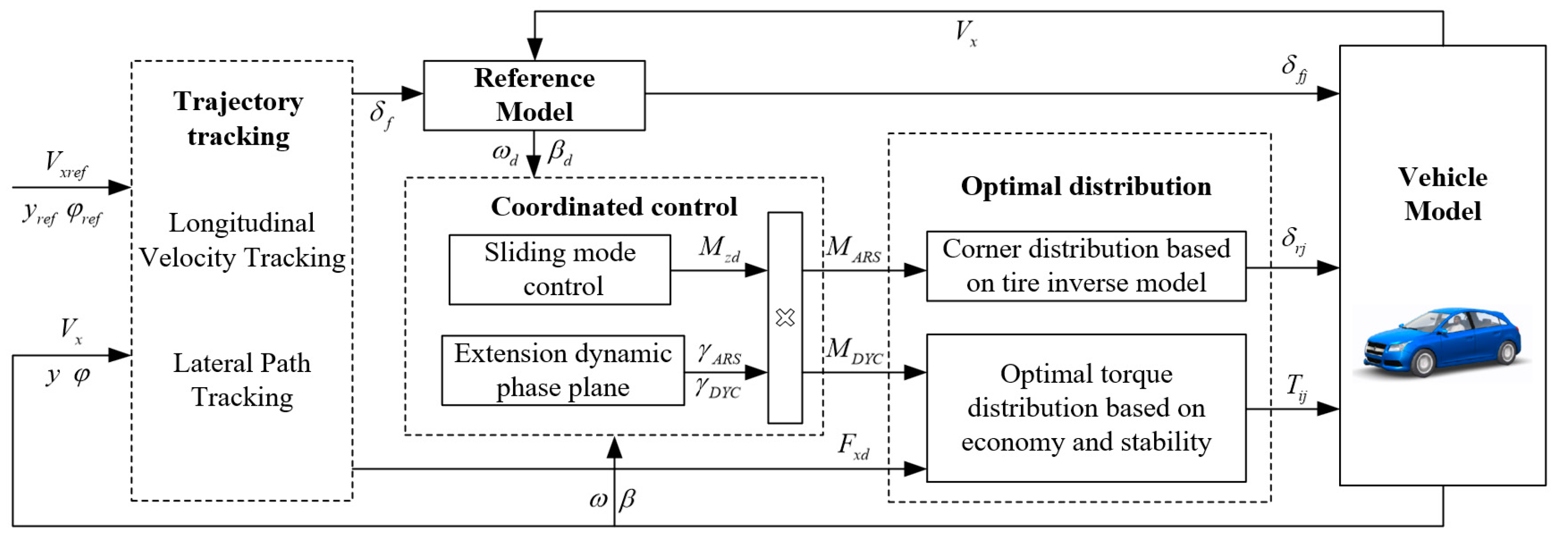
• A hierarchical chassis coordinated control architecture is proposed, consisting of a trajectory tracking layer, coordinated control layer, and optimal distribution layer, taking into account trajectory tracking performance, handling stability, and economy.
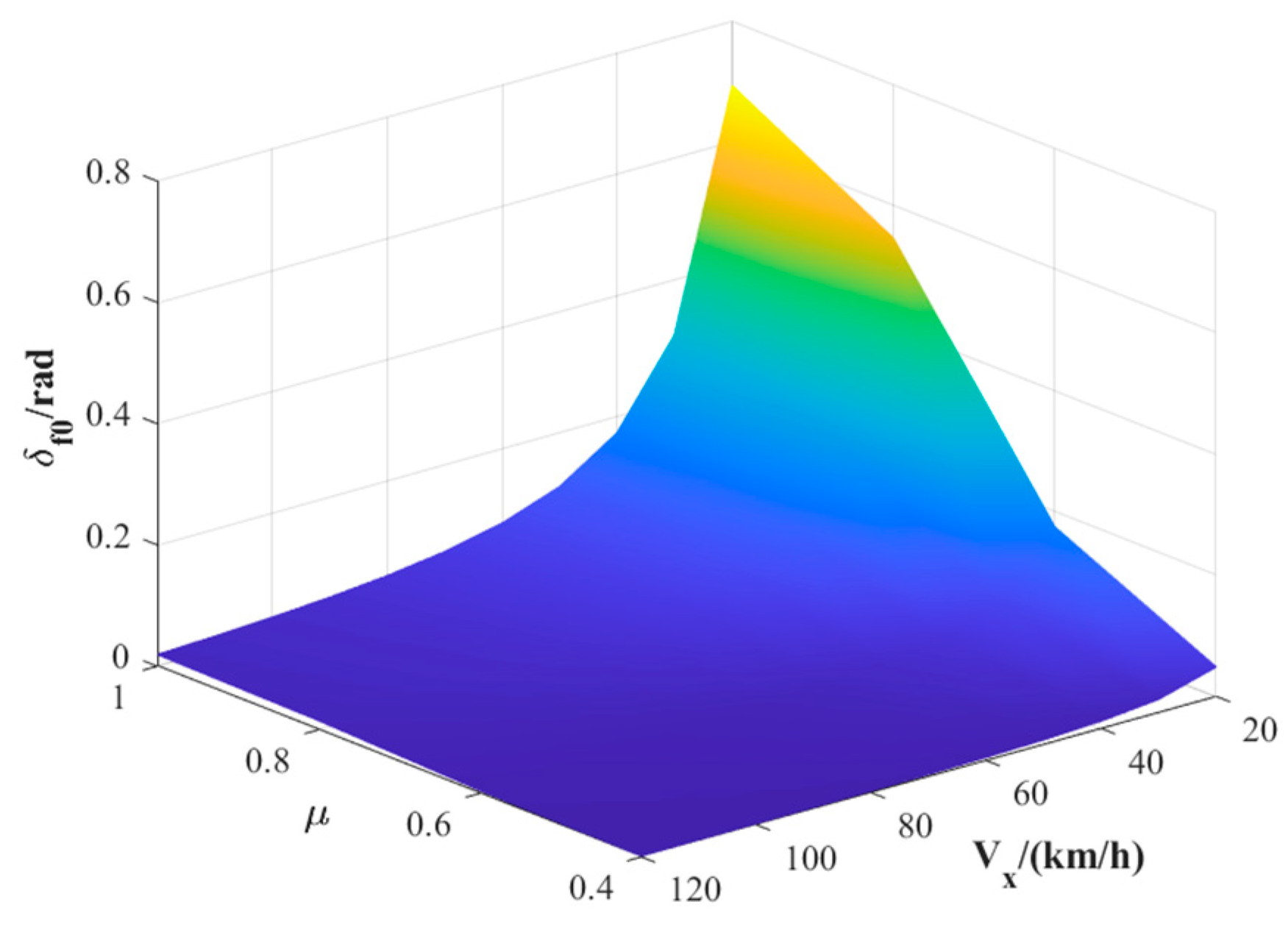
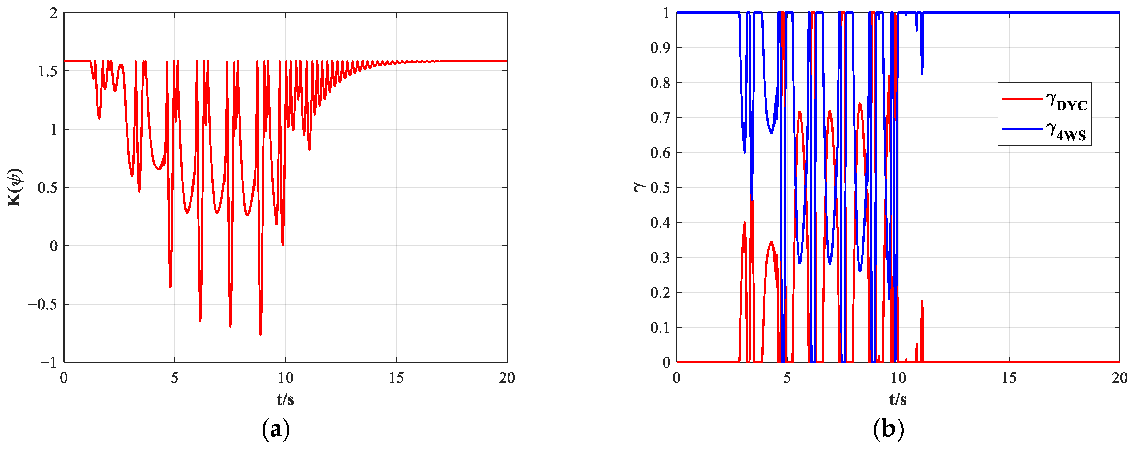
• The extension theory is employed to extend the traditional phase plane, constructing an extension dynamic stability domain based on the vehicle’s linear response characteristics. The boundary values of the extension domain are adaptively adjusted according to vehicle speed and road adhesion coefficient, determining the control weights for ARS and DYC. This method is simple and efficient, overcoming the limitations of traditional stability domain boundaries that cannot be adjusted and are difficult to accurately obtain.
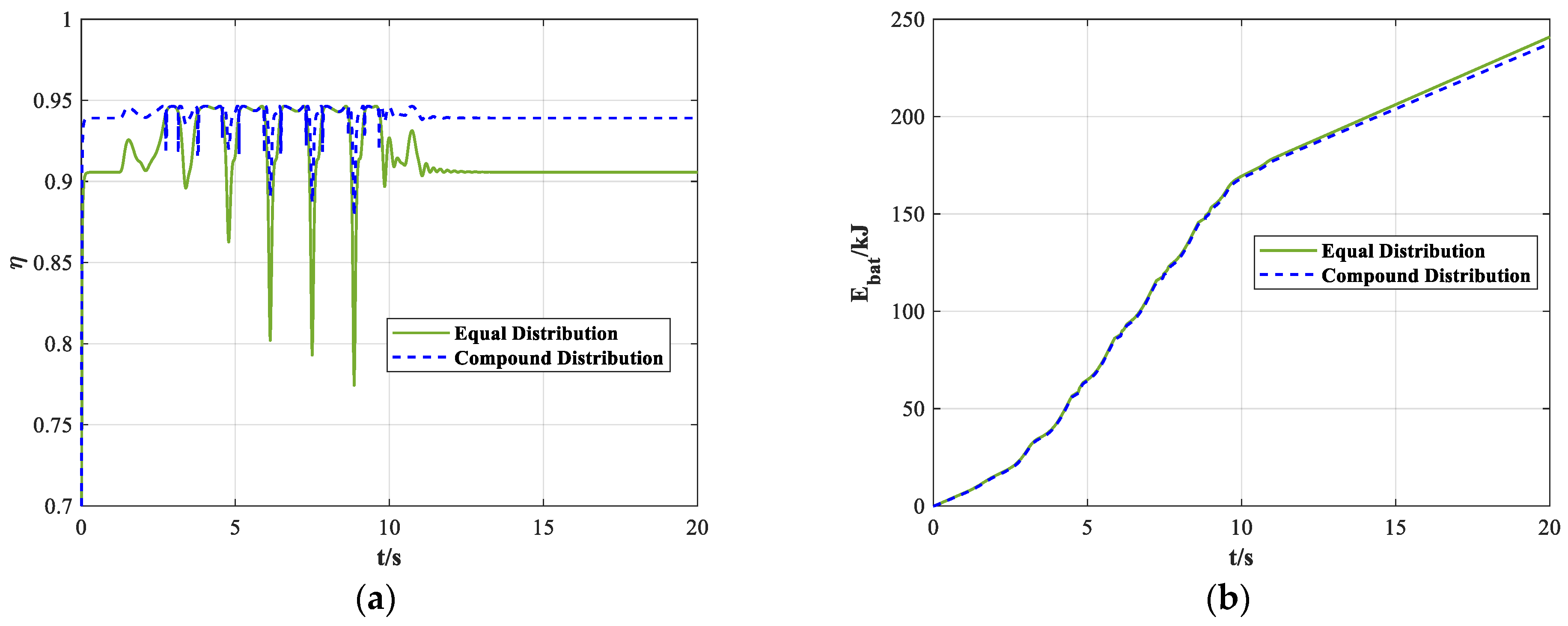
• A compound torque distribution strategy is developed that combines economic distribution with stability distribution, taking into account driving efficiency and tire adhesion rate as indicators. The real-time optimal distribution of wheel torque is achieved using the mutant particle swarm algorithm (MPSO) and the quadratic programming algorithm, respectively. It demonstrates good real-time performance and enables multi-objective optimization of stability and economy.

The paper is organized as follows: Section 2 proposes a hierarchical chassis coordinated control strategy. Section 3 performs simulation validation. Section 4 compares and discusses the simulation results. Section 5 reaches the conclusions.

2. Chassis Coordinated Control

2.1. Vehicle Model

To investigate the chassis coordinated control strategy of 4WID-4WIS EVs, the dynamic modeling of the vehicle, tires, and motor is performed based on the nonlinearity of the tire and the efficiency characteristics of the motor.

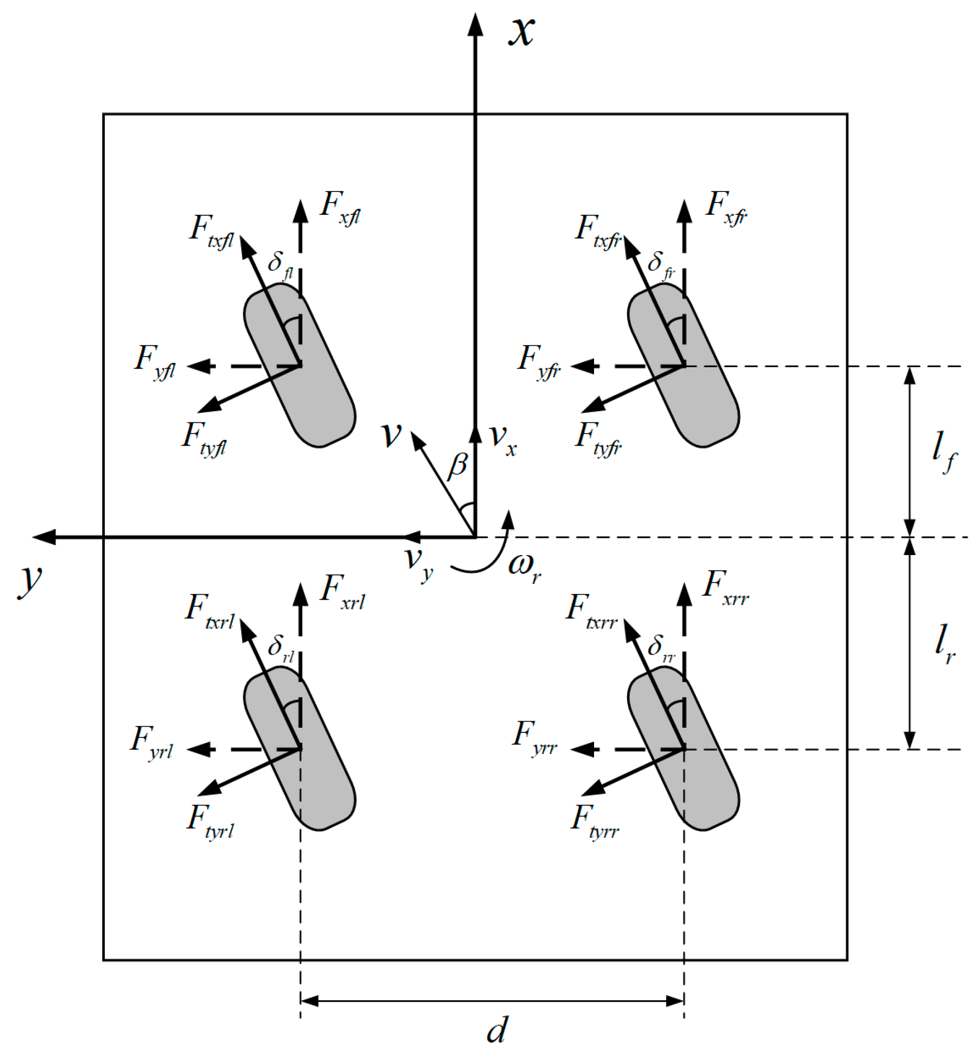
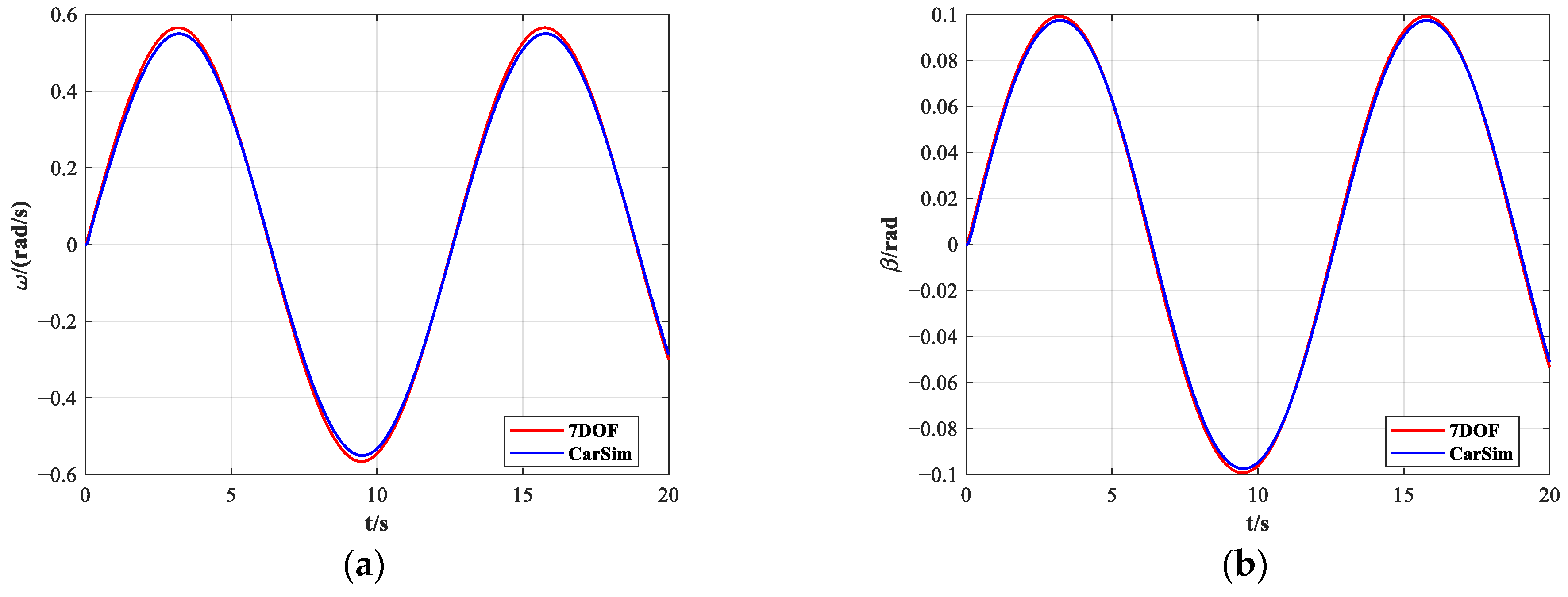
2.1.1. Vehicle Dynamic Model

Various scholars have proposed different linear and nonlinear vehicle models of varying complexity to investigate vehicle dynamics control problems [26]. This research primarily focuses on the control of lateral and longitudinal coupling for trajectory tracking. A 7-DOF vehicle dynamic model is utilized, which includes longitudinal motion, lateral motion, yaw motion, and the rotation of the four wheels based on the distributed drive system.

The vehicle under study has a small mass, compact dimensions, and a low center of gravity. Therefore, when establishing the vehicle dynamic model, it is assumed that the vehicle is symmetric about the center plane and is traveling on a flat horizontal road. The vertical motion of the body is neglected. Additionally, the suspension system is regarded as a rigid structure, ignoring the pitch and roll movements. After these simplifications, the dynamic model is shown in Figure 1.

The longitudinal motion equation is

$$m\left({\dot{v}}_x-v_y{\omega }_r\right)=F_{xfl}+F_{xfr}+F_{xrl}+F_{xrr}$$

(1)

The lateral motion equation is

$$m\left({\dot{v}}_y+v_x{\omega }_r\right)=F_{yfl}+F_{yfr}+F_{yrl}+F_{yrr}$$

(2)

The equation of yaw motion is

$$I_z{\dot{\omega }}_r=\left(F_{xfr}+F_{xrr}-F_{xfl}-F_{xrl}\right)\frac{d}{2}+\left(F_{yfl}+F_{yfr}\right)l_f-\left(F_{yrl}+F_{yrr}\right)l_r$$

(3)

where

$$F_{xij}=F_{txij}\cos {\delta }_{ij}-F_{tyij}\sin {\delta }_{ij}$$

(4)

$$F_{yij}=F_{txij}\sin {\delta }_{ij}+F_{tyij}\cos {\delta }_{ij}$$

(5)

$$i\in \left\{f,r\right\},j\in \left\{l,r\right\}$$

(6)

The equation of wheel motion is

$$I_w{\dot{\omega }}_{ij}=T_{dij}-F_{txij}{R}_{eff}-T_{bij}$$

(7)

where $v_x$ and $v_y$ are the longitudinal velocity and lateral velocity; ${\omega }_r$ is the yaw rate; $F_{xij}$ and $F_{yij}$ are the longitudinal force and lateral force of each wheel, respectively; $F_{txij}$ and $F_{tyij}$ are the longitudinal and lateral forces of each wheel in the tire coordinate system; ${\delta }_{ij}$ is the wheel angle; $I_w$ is the wheel moment of inertia; ${\omega }_{ij}$ is the wheel speed; $T_{dij}$ is the wheel driving torque; and $T_{bij}$ is the wheel braking torque.

To validate the effectiveness of the constructed 7-DOF model, a comparison is made with the vehicle model in the CarSim 2019. The simulation parameters are set as follows: the vehicle speed is set to 60 km/h, the road adhesion coefficient is set to 0.8, and the steering wheel input is set to a sinusoidal steering angle signal.

The model validation results are shown in Figure 2. The yaw rate and sideslip angle results obtained from the 7-DOF model are basically the same as those from the CarSim vehicle model, meeting the model accuracy requirements. This confirms the effectiveness of the 7-DOF vehicle model.

2.1.2. Tire Model

The tire model describes the relationship between the tire’s motion parameters and tire forces. It can be broadly classified into three types: theoretical models, empirical models, and semi-empirical models [27]. Considering the tire’s side slip characteristics, this research selects the widely used UniTire semi-empirical tire model. The UniTire tire model takes into account various factors such as longitudinal slip, lateral slip, camber, turning angle, and hysteresis effects on tire force generation. It is characterized by high simulation accuracy, strong predictive capability, and well-defined theoretical boundaries. The longitudinal slip ratio and lateral slip ratio are defined as follows:

$$\left\{\begin{array}{l}{S}_x=\frac{{\nu }_{sx}}{\omega r}\\ S_y=\frac{{\nu }_{sy}}{\omega r}=\left(1+S_x\right)\tan \alpha \end{array}\right.$$

(8)

where $\alpha$ is the tire slip angle.

The dimensionless relative longitudinal slip ratio, lateral slip ratio, and total slip ratio are defined as follows:

$$\left\{\begin{array}{l}{\mathsf{\varphi }}_x=\frac{K_x{S}_x}{{\mu }_x{F}_z}\\ {\mathsf{\varphi }}_y=\frac{K_y\tan \alpha }{{\mu }_y{F}_z}\\ {\mathsf{\varphi }}_n=\sqrt{{(k_u{\mathsf{\varphi }}_x)}^2+{\mathsf{\varphi }}_y^2}\end{array}\right.$$

(9)

where $K_x$ and $K_y$ are the longitudinal and lateral stiffness of the tire, respectively; ${\mu }_x$ and ${\mu }_y$ are the longitudinal and lateral friction coefficients between the tire and the ground, respectively; and $k_u$ is the correction factor that accounts for the difference in longitudinal and lateral stiffness of the tire.

In combined longitudinal and lateral slip conditions, the UniTire tire model accurately describes the dimensionless total shear force using the exponential form

$${\overline{F}}_n=1-\exp (-{\mathsf{\varphi }}_n-E·{\mathsf{\varphi }}_n^2-(E^2+\frac{1}{12})·{\mathsf{\varphi }}_n^3)$$

(10)

The dimensionless total shear force is distributed into dimensionless longitudinal force and dimensionless lateral force based on the proportion of dimensionless relative longitudinal and lateral slip ratios in the dimensionless total slip ratio.

$$\left\{\begin{array}{l}{\overline{F}}_x={\overline{F}}_n\frac{k_u{\mathsf{\varphi }}_x}{{\mathsf{\varphi }}_n}\\ {\overline{F}}_y={\overline{F}}_n\frac{{\mathsf{\varphi }}_y}{{\mathsf{\varphi }}_n}\end{array}\right.$$

(11)

The longitudinal and lateral forces on the tire are

$$\left\{\begin{array}{c}{F}_x={\overline{F}}_x{\mu }_x{F}_z\\ F_y={\overline{F}}_y{\mu }_y{F}_z\end{array}\right.$$

(12)

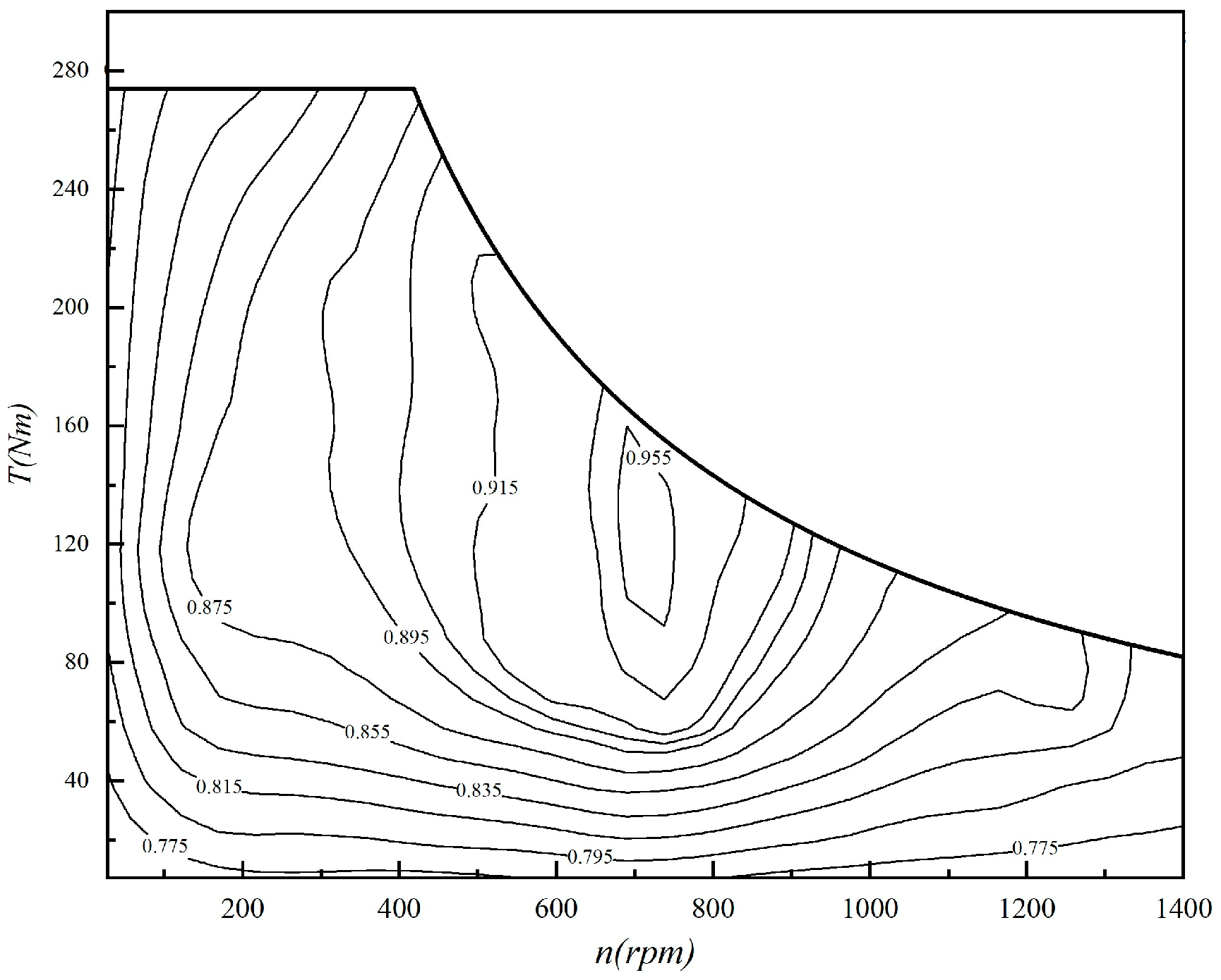
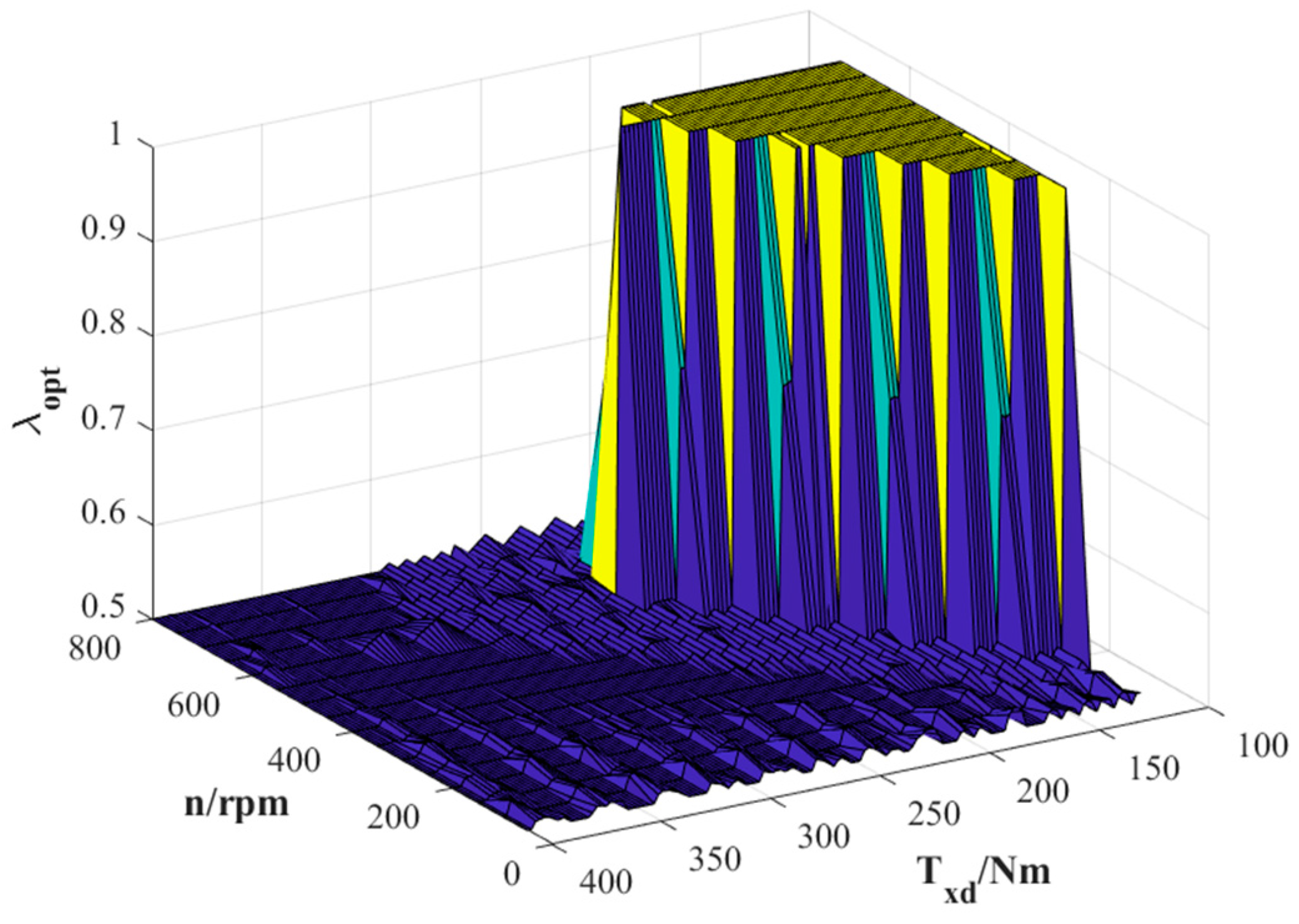
2.1.3. Motor Model

The 4WID-4WIS EV chassis system consists of in-wheel motors and steering motors. Based on the vehicle’s economy and handling stability performance requirements, and combined with the efficiency and dynamic characteristics of the motor, separate models are established for in-wheel motors and steering motors.

• In-wheel motor model:

In order to investigate the energy efficiency of the chassis, this study develops a motor energy efficiency model that takes into account the efficiency characteristics of the in-wheel motor. To simplify the computation, this research focuses solely on the steady-state characteristics of the motor, disregarding the transient characteristics and simplifying the charging and discharging efficiency. Therefore, the efficiency model can be represented as Equation (13).

$${\eta }_{em}=\eta \left(n_{em},T_{em}\right)$$

(13)

where $n_{em}$ is the motor speed, and $T_{em}$ is the motor torque.

The efficiency characteristics of the in-wheel motor’s driving efficiency are depicted using external characteristic curves and efficiency maps, as illustrated in Figure 3. The external characteristic curve sets the upper limit of the motor’s maximum output power. Additionally, the motor’s discharge efficiency can be assessed in real time by referring to a two-dimensional lookup table of the motor efficiency map. This allows for a comprehensive study of the economy of the drive system.

2.

Steering motor model

In order to meet the dynamic response requirements during vehicle driving, the steering motor model is simplified into a corner tracking model, the delay caused by the steering mechanism is considered, and a model shown in Equation (14) is established:

$${\delta }_{ij\_out}={\delta }_{ij\_req}·\frac{1}{1+\tau s}$$

(14)

where ${\delta }_{ij\_out}$ is the actual output angle, ${\delta }_{ij\_req}$ is the required output angle, and $\tau$ is the response time constant.

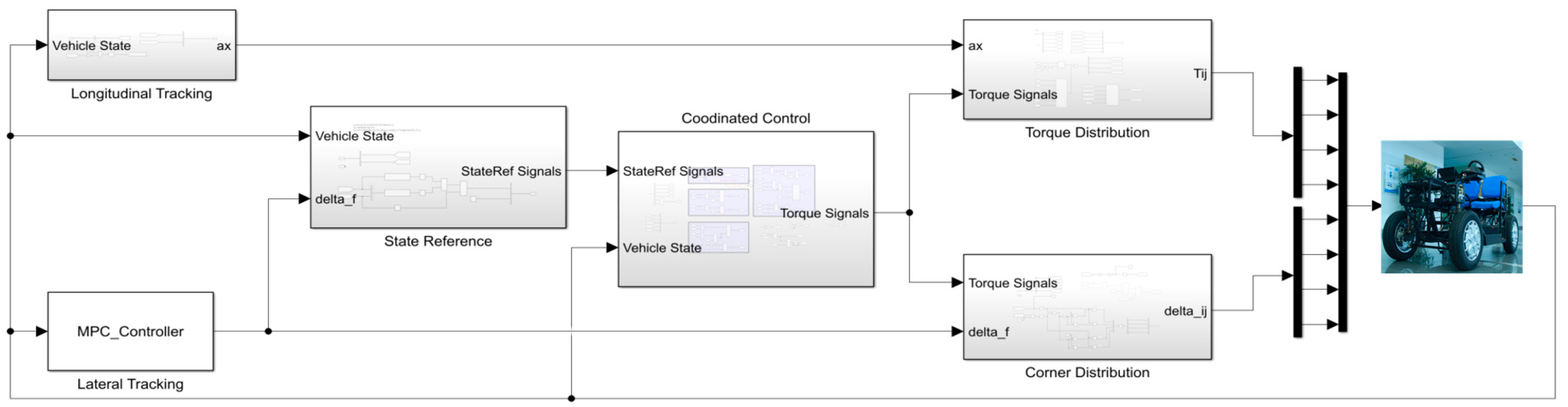
2.2. Chassis Control Architecture

Intelligent driving vehicles receive trajectory information from the planning layer and use rational control strategies to achieve trajectory tracking control, fulfilling the functional goals of autonomous driving. Vehicles with four-wheel independent drive and four-wheel independent steering (4WID-4WIS EVs) have multiple degrees of freedom, which significantly expands the control margin of chassis dynamics and increases the upper limit of the chassis stability domain. This potential allows for the improvement in vehicle performance and serves as a basis for the multi-objective coordinated control of the chassis. Therefore, this research aims to leverage the control advantages of the fully wired chassis to enhance handling stability and economy during the trajectory tracking process.

The designed chassis coordinated control architecture Is shown in Figure 4, employing a layered strategy structure that includes a trajectory tracking layer, coordinated control layer, and optimal distribution layer.

Based on a decentralized control structure, the trajectory tracking layer separates the longitudinal and lateral control targets, converting the desired trajectory information into vehicle input information. The expert PID control method is employed to track the desired vehicle speed and generate the expected longitudinal acceleration. The MPC controller is responsible for tracking the desired path and producing the expected front wheel angle.

The coordinated control layer calculates the expected actions of the subsystems based on the anticipated vehicle state. Sliding mode control is used to compute the generalized yaw moment and incorporates an adaptive adjustment strategy for the control weights of ARS and DYC. This strategy is designed considering the extension dynamic stability domain and allocates the desired yaw moment, determining the control objectives for the ARS and DYC.

The optimal distribution layer designs torque distribution and corner distribution strategies, converting the expected subsystem actions into control commands for actuators. The optimal torque distribution control strategy based on economy and stability is adopted, using driving efficiency and tire adhesion rate as control indicators for economy and stability, respectively. It computes the optimal driving torque for each wheel via a combination of MPSO and DP. The corner distribution strategy employs the tire inverse model to calculate the tire slip angle. Combined with the Ackermann steering theory, the steering angle for each wheel is output to achieve the vehicle’s closed-loop control.

2.3. Trajectory Tracking Layer

The trajectory tracking layer’s main objective is to replace the driver in following the desired trajectory by providing the desired longitudinal acceleration and front wheel angle. This layer takes into account the desired path and vehicle speed, which are the combined desired longitudinal and lateral motion states of the vehicle. As a result, the trajectory tracking problem is divided into two separate problems: longitudinal velocity tracking and lateral path tracking. By calculating the expected longitudinal acceleration and front wheel angle independently, this layer is able to provide the necessary inputs for the coordinated control of the chassis.

2.3.1. Longitudinal Velocity Tracking

Proportional integral derivative (PID) control is widely applied in longitudinal vehicle speed tracking due to its simplicity, practicality, and independence from precise system models. Given the uncertainty of system parameters, external disturbances, and nonlinear couplings between subsystems, many researchers have explored PID control based on intelligent algorithms [28,29]. In this study, based on expert system theory, the expert PID is employed for longitudinal velocity tracking. The specific algorithm flow can be found in [30]. The calculation formula for longitudinal acceleration is as follows:

$$a_{xd}=u(k)=\left\{\begin{array}{c}\begin{array}{c}{a}_{x\max }\\ u(k-1)+k_1\left\{k_{i}e(k)+k_p\mathsf{\Delta }e(k)+k_d\mathsf{\Delta }e(k)\right\}\end{array}\\ u\left(k-1\right)\\ u(k-1)+k_2{k}_{i}e(k)\\ u(k-1)+k_{i}e(k)+k_p\mathsf{\Delta }e(k)\end{array}\right.\begin{array}{c}\begin{array}{c}(\left|e\left(k\right)\right|>M_{max})\\ (e\left(k\right)\times \mathsf{\Delta }e\left(k\right)>0 \mathrm{or} \mathsf{\Delta }e\left(k\right)=0)\end{array}\\ (e(k)\mathsf{\Delta }e(k)<0, \mathsf{\Delta }e(k)\mathsf{\Delta }e(k-1)>0, e(k)=0)\\ (e(k)\mathsf{\Delta }e(k)<0, \mathsf{\Delta }e(k)\mathsf{\Delta }e(k-1)<0)\\ (\left|e\left(k\right)\right|<M_{min})\end{array}$$

(15)

where $e(k)=v(k)-v_d(k)$ is the velocity error, and $e(k)=v(k)-v_d(k)$ is the velocity error increment. The maximum deviation value is set as $M_{max}$, the middle deviation value is set as $M_{mid}$, and the minimum deviation value is set as $M_{min}$.

Ignoring the road gradient resistance and considering rolling resistance, aerodynamic resistance, and acceleration resistance, a feedforward controller is designed according to the longitudinal vehicle dynamics equation as follows:

$$F_{xd}=F_f+F_{air}+F_j=mgf+\frac{C_{D}A{\nu }_x^2}{21.15}+m{a}_{xd}$$

(16)

where $F_{xd}$ is the generalized longitudinal force, $F_f$ is the rolling resistance, $F_{air}$ is the air resistance, $F_j$ is the acceleration resistance, $f$ is the rolling resistance coefficient, $C_D$ is the air resistance coefficient, and $A$ is the windward area.

2.3.2. Lateral Path Tracking

In order to navigate complex and ever-changing driving environments, autonomous vehicles need to take into account road constraints, safety constraints, and actuator constraints while tracking their trajectory. Model predictive control (MPC) is a widely used feedback control algorithm that predicts future system outputs based on the current model and state and solves a finite-time open-loop optimization problem on a rolling basis to achieve control objectives. MPC has proven to be highly effective in handling multi-constraint optimization problems. As a result, scholars have conducted extensive research on the application of MPC-based lateral path tracking control in recent years [29]. This study utilizes MPC to achieve lateral path tracking.

The accuracy of the prediction model directly impacts the control effectiveness of MPC. To balance the requirements of accuracy and complexity, a nonlinear 3-DOF vehicle model is chosen as the prediction model to forecast the system’s output. The state variable is $X={\left[v_x,v_y,\phi ,\dot{\phi },x,y\right]}^T$, the control variable is $u={\left[{\delta }_f\right]}^T$, and the output variable is $Y={\left[\phi ,y\right]}^T$. Assuming constant longitudinal velocity during path tracking and to meet the real-time requirements of high-speed control, this paper linearizes the nonlinear system using Taylor’s formula. Simultaneously, a discretization process is applied to obtain the control system model:

$$\begin{array}{c}X\left(k+1\right)=A_{dyn}\left(k\right)X\left(k\right)+B_{dyn}\left(k\right)u\left(k\right)\\ Y\left(k\right)=CX\left(k\right)\end{array}$$

(17)

where

$$A_{dyn}\left(k\right)=\left[\begin{array}{cccccc}\frac{C_{\alpha f}+C_{\alpha r}}{m\dot{x}}& -\dot{\phi }-\frac{\left(C_{\alpha f}+C_{\alpha r}\right)\dot{y}-\left(l_r{C}_{\alpha r}-l_f{C}_{\alpha f}\right)\dot{\phi }}{m{\dot{x}}^2}& 0& -\dot{x}+\frac{l_f{C}_{\alpha f}-l_r{C}_{\alpha r}}{m\dot{x}}& 0& 0\\ \dot{\phi }+\frac{C_{\alpha f}{\delta }_f}{m\dot{x}}& -\frac{C_{\alpha f}{\delta }_f\left(\dot{y}+l_f\dot{\phi }\right)}{m{\dot{x}}^2}& 0& \dot{y}+\frac{l_f{C}_{\alpha f}{\delta }_f}{m\dot{x}}& 0& 0\\ 0& 0& 0& 0& 0& 0\\ \frac{l_f{C}_{\alpha f}-l_r{C}_{\alpha r}}{I_z\dot{x}}& -\frac{\left(l_f{C}_{\alpha f}-l_r{C}_{\alpha r}\right)\dot{y}+\left(l_f^2{C}_{\alpha f}+l_r^2{C}_{\alpha r}\right)\dot{\phi }}{I_z{\dot{x}}^2}& 0& \frac{l_f^2{C}_{\alpha f}+l_r^2{C}_{\alpha r}}{I_z\dot{x}}& 0& 0\\ \cos \phi & \sin \phi & \dot{x}\cos \phi -\dot{y}\sin \phi & 0& 0& 0\\ -\sin \phi & \cos \phi & -\dot{x}\sin \phi -\dot{y}\cos \phi & 0& 0& 0\end{array}\right]$$

(18)

$$B_{dyn}\left(k\right)={\left[-\frac{C_{\alpha f}}{m}\hspace{1em}\frac{C_{\alpha f}\left[\left(\dot{y}+l_f\dot{\phi }\right)-2{\delta }_f\dot{x}\right]}{m\dot{x}}\hspace{1em}0\hspace{1em}-\frac{l_f{C}_{\alpha f}}{I_z}\hspace{1em}0\hspace{1em}0\right]}^T$$

(19)

$$C=\left[\begin{array}{cccccc}0& 0& 1& 0& 0& 0\\ 0& 0& 0& 0& 1& 0\end{array}\right]$$

(20)

where $\phi$ is the heading angle, $C_{\alpha f}$ and $C_{\alpha r}$ are the equivalent cornering stiffnesses of the front axle and the rear axle, respectively, and $x$ and $y$ are the longitudinal and lateral coordinates of the centroid in the geodetic coordinate system, respectively.

The control objectives are defined based on the tracking accuracy of the reference path and the smooth variation in control inputs. The tracking accuracy is assessed using lateral offset and heading angle error as evaluation metrics. Therefore, the design of the performance evaluation function is as follows:

$$J={\left[Y_p\left(k\right)-Y_{ref}\right]}^T{Q}_Q\left[Y_p\left(k\right)-Y_{ref}\right]+\mathsf{\Delta }U{\left(k\right)}^T{R}_R\mathsf{\Delta }U\left(k\right)$$

(21)

where $Q_Q=I_p\otimes Q$, $R_R=I_c\otimes R$, $Q$ is the weight coefficient matrix of the output of the control system, $R$ is the weight coefficient matrix of the control increment, and $\otimes$ represents the Kronecker product.

During the solving process, three aspects need to be considered: control increment constraints, control quantity constraints, and stability constraints.

To ensure a smoother control process and enhance stability and comfort while tracking the desired path, constraints are applied to the control increment, as shown in Equation (22):

$$\mathsf{\Delta }{U}_{\min }\left(k\right)\le \mathsf{\Delta }U\left(k\right)\le \mathsf{\Delta }{U}_{\max }\left(k\right)$$

(22)

Due to limitations in the actuators, there are constraints on the control quantity for the front wheel angle, represented as

$$u_{\min }\left(k\right)\le u\left(k\right)\le u_{\max }\left(k\right)$$

(23)

To ensure that the vehicle has good stability, constraints are imposed on the lateral yaw rate and tire slip angle. The constraint on the lateral yaw rate due to road conditions is as follows:

$$-\frac{\mu g}{v_x}\le {\omega }_r\le \frac{\mu g}{v_x}$$

(24)

When the vehicle becomes unstable, the consequences of rear axle sideslip are more severe. So, the rear wheel slip angle needs to be restrained; that is

$${\alpha }_{r,\min }\le {\alpha }_r\le {\alpha }_{r,\max }$$

(25)

By solving the QP problem, the optimal control increment sequence $\mathsf{\Delta }{U}^{\ast }\left(k\right)$ is obtained. The first element $\mathsf{\Delta }{u}^{\ast }\left(k\right)$ is applied to the controlled system and converted into the control quantity at the present moment, which provides the desired front wheel angle.

$${\delta }_f=u\left(k\right)=u\left(k-1\right)+\mathsf{\Delta }{u}^{\ast }\left(k\right)$$

(26)

2.4. Coordinated Control Layer

The coordinated control layer calculates the expected vehicle state by using the output of the trajectory tracking layer, which provides the expected vehicle action. To track the desired state, a sliding mode controller is designed to generate the expected vehicle effect. Furthermore, this research explores a coordinated control strategy based on the theory of extension dynamic phase plane. This strategy aims to improve the vehicle’s handling stability and coordinate the coupling between the steering and drive subsystems. It achieves this by allocating the expected yaw moment and calculating the desired control objectives for the steering and drive systems.

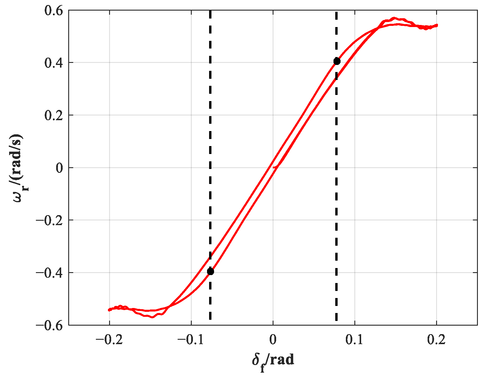
2.4.1. Reference States

The handling stability of a vehicle’s lateral motion is determined by two important parameters: yaw rate and sideslip angle. The yaw rate affects the quality of the vehicle’s dynamic response. If the yaw rate is too large, it may cause oversteer, while if it is too small, it may result in understeer. On the other hand, the sideslip angle reflects how much the vehicle deviates from its intended path during driving. A larger sideslip angle indicates a greater deviation in path tracking. Therefore, to ensure handling stability, it is essential to set appropriate values for the yaw rate and sideslip angle.

Based on the 2-DOF model of a front wheel steering vehicle, the expected yaw rate can be obtained by calculating the steady-state response of the yaw rate:

$${\omega }_d=\frac{{\delta }_f{V}_x}{L+\frac{\mathrm{m}{V}_x^2(l_f{C}_{\alpha f}-l_r{C}_{\alpha r})}{L{C}_{\alpha f}{C}_{\alpha r}}}$$

(27)

Considering the road adhesion constraints, the expected yaw rate can be represented as

$${\omega }_d=\min \{\left|{\omega }_d\right|,\left|0.85\frac{\mu g}{v_x}\right|\}\mathrm{sgn}({\delta }_f)$$

(28)

The expected side slip angle can also be calculated via the steady-state response of the 2-DOF vehicle model. However, to simplify the calculation, the expected side slip angle is set to be 0 rad.

2.4.2. Additional Yaw Moment

For both the 4WID system and the 4WIS system, the control objectives for handling stability include tracking the expected yaw rate and the expected side slip angle. Therefore, this paper adopts sliding mode control to track these two reference states. It calculates the additional yaw moment required to meet the tracking task, transforming the desired vehicle state into the desired vehicle action, thus achieving the objectives of improving chassis maneuverability and stability.

The sliding surface of the tracking error is set as follows:

$$s=\omega -{\omega }_d+\rho (\beta -{\beta }_d)$$

(29)

where $\rho$ represents the weight coefficient of the sideslip angle.

The yaw rate and side slip angle are control objectives that characterize vehicle stability. However, in many cases, it is challenging to simultaneously achieve both objectives. The yaw rate indicates whether the vehicle is understeering or oversteering, which directly impacts its handling performance. On the other hand, the side slip angle measures the deviation of the vehicle’s trajectory during steering, thereby affecting its lateral stability. Consequently, the coupling between the yaw rate and side slip angle becomes a crucial aspect when calculating the desired vehicle action. Currently, the phase plane method is considered one of the effective approaches to address this coupling problem. The phase plane index is defined as follows:

$$X_{\mathrm{region}}=\left|B_1\dot{\beta }+B_2\beta \right|$$

(30)

where $B_1$ and $B_2$ are the boundary model coefficients.

Within the stable region of the phase plane, the phase trajectory of the side slip angle can automatically converge to zero, which imparts trajectory-following characteristics and lateral stability to the car. As a result, the primary control objective is to achieve the desired yaw rate. However, outside the stable region, the phase trajectory of the side slip angle diverges, leading to vehicle instability. In such cases, both the desired yaw rate and side slip angle become the main control objectives. Furthermore, as the phase plane index increases, the weight of the side slip angle gradually increases. So, the weight coefficient is defined as

$$\rho =\left\{\begin{array}{ll}0\hfill & X_{\mathrm{region}}⩽0.8\hfill \\ (X_{\mathrm{region}}-0.8)\times 5k\hfill & 0.8⩽X_{\mathrm{region}}⩽1\hfill \\ k\hfill & X_{\mathrm{region}}⩾1\hfill \end{array}\right.$$

(31)

where $k$ is a positive number.

The vehicle 2-DOF model is used as the control model:

$$\left\{\begin{array}{l}\dot{\omega }=\frac{l_f{C}_{\alpha f}}{I_z}\left(\beta +\frac{l_f\omega }{V_x}-{\delta }_f\right)-\frac{l_r{C}_{\alpha r}}{I_z}\left(\beta -\frac{l_r\omega }{V_x}\right)+\frac{M}{I_z}\\ \dot{\beta }=-\omega +\frac{C_{\alpha f}}{m{V}_x}(\beta +\frac{l_f\omega }{V_x}-{\delta }_f)+\frac{C_{\alpha r}}{m{V}_x}(\beta -\frac{l_r\omega }{V_x})\end{array}\right.$$

(32)

During the control process, the presence of inertia and hysteresis can lead to chattering, which has a significant impact on the system’s performance. To attenuate chattering and enhance system stability, this research employs an exponential reaching law with a saturation function, as shown in the following equation:

$$\dot{s}=-\epsilon ·sat\left(s/\varphi \right)-ks$$

(33)

where, $\epsilon >0$, $k>0$, $\varphi >0$, and

$$sat\left(\frac{s}{\varphi }\right)=\left\{\begin{array}{ll}1,& s>\varphi \\ \frac{s}{\varphi },& \left|s\right|\le \varphi \\ -1,& s<-\varphi \end{array}\right.$$

(34)

According to Equations (30), (32) and (33), the additional yaw moment can be calculated as follows:

$$\begin{array}{l}{M}_{zd}=I_z\{(-\epsilon ·sat\left(s/\varphi \right)-ks)+l_f{C}_{\alpha f}\left({\delta }_f-\beta -\frac{l_f\omega }{V_x}\right)-l_r{C}_{\alpha r}\left(-\beta +\frac{l_r\omega }{V_x}\right)+I_z{\dot{\omega }}_{rd}\\ -I_z\rho \{(-\omega +\frac{C_{\alpha f}}{m{V}_x}(\beta +\frac{l_f\omega }{V_x}-{\delta }_f)+\frac{C_{\alpha r}}{m{V}_x}(\beta -\frac{l_r\omega }{V_x})-{\dot{\beta }}_d\}\end{array}$$

(35)

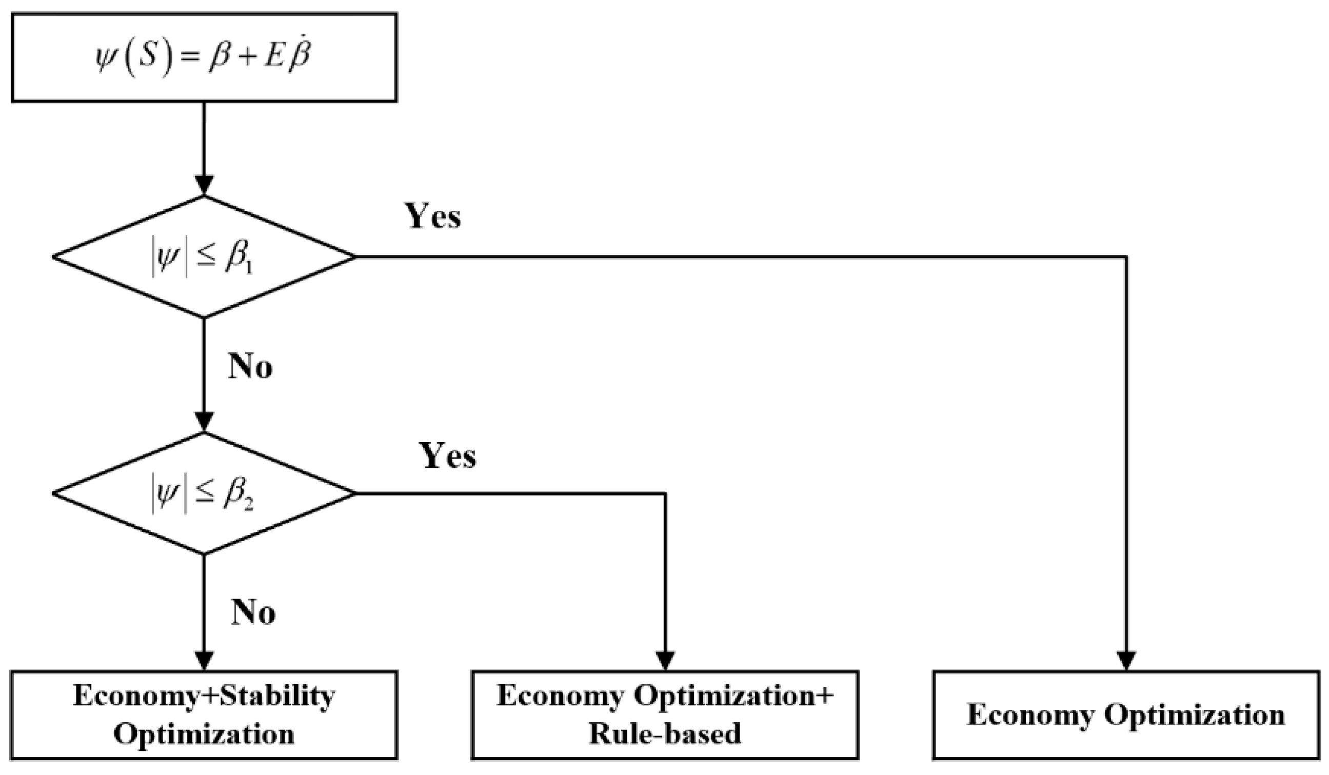
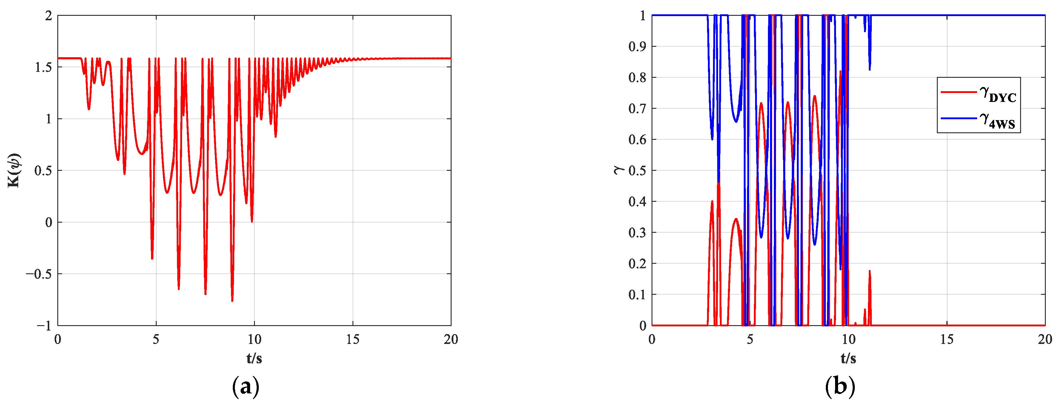
2.4.3. Coordinated Strategy

To address the limitations of the traditional phase plane, this research introduces the extension theory to expand the stability domain of the original phase portrait. Additionally, the dynamic boundaries for the extension domain are designed by considering the linear response characteristics of the vehicle. These boundary values can be dynamically adjusted based on factors such as vehicle speed and road adhesion coefficient, which helps overcome the issues associated with fixed domain boundaries and poor adaptability observed in existing research. By utilizing the extension dynamic phase portraits, the lateral states of the vehicle are categorized into three regions: classical domain, extension domain, and non-domain. Different allocation strategies are applied to each region to distribute the expected additional yaw moments. Furthermore, the control weights of DYC and ARS are adaptively adjusted, and the target yaw moments for DYC and ARS are calculated and outputted.

The control strategy based on the extension dynamic stability domain is mainly divided into several parts, including characteristic state extraction, domain division, correction calculation, and measurement pattern recognition.

• Characteristic State Extraction:

According to the definition expansion of the extension primitive theory, the characteristic quantity can represent the state characteristic variables that describe the system control objectives. The phase plane of the side slip angle and its angular velocity can reflect the vehicle’s lateral stability, and it is widely used. Therefore, $\mathcal{S}\left(\beta ,\mathrm{d}\beta \right)$ is selected as the characteristic state. A two-dimensional extension set is established to describe the stable driving state.

2.

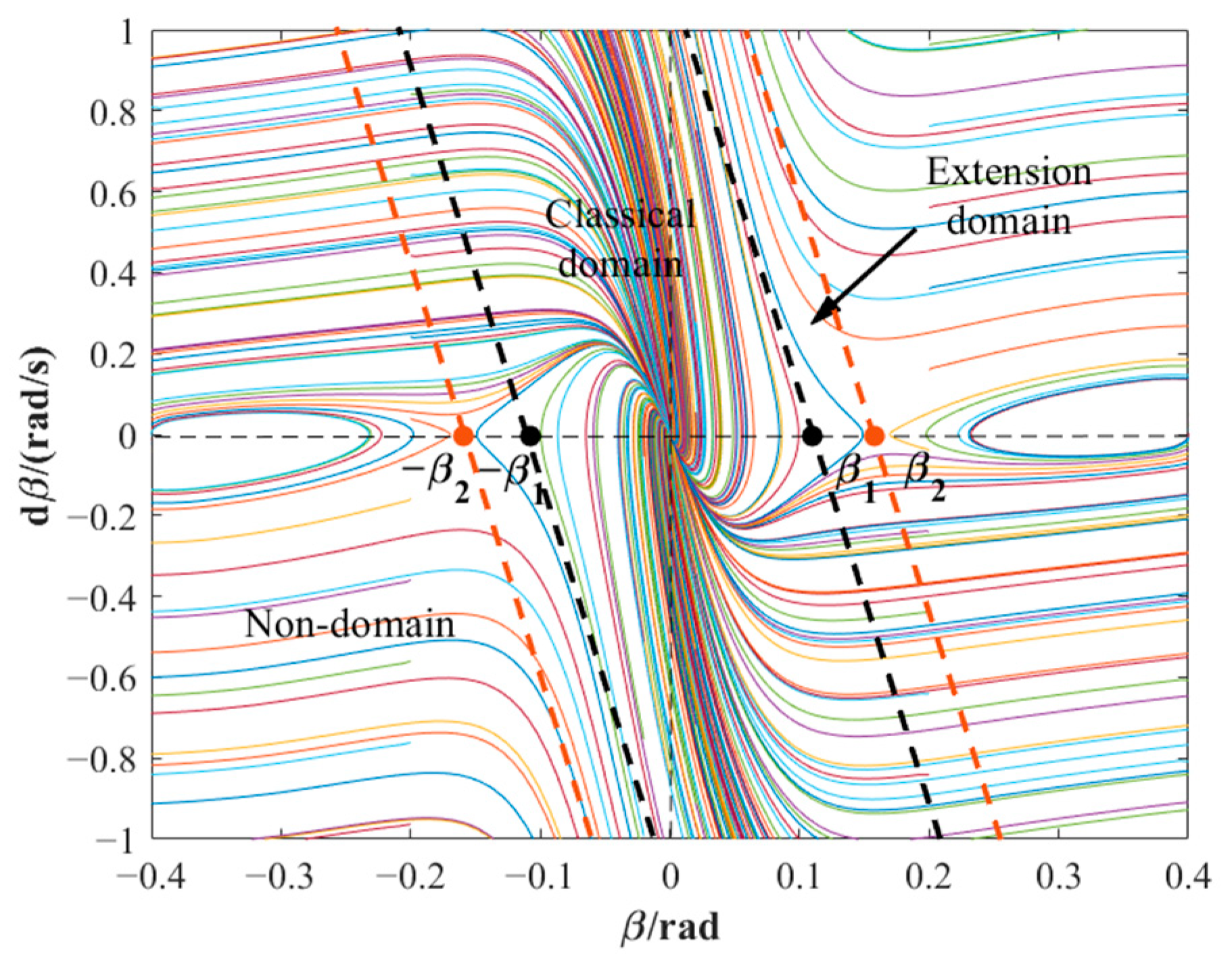
Domain Division

In this research, a dual-line method is used to divide the original phase portrait into three regions: classical domain, extension domain, and non-domain, as shown in Figure 5. The classical domain represents the stable state, the extension domain represents the critical stable state, and the non-domain represents the unstable state. Therefore, accurately determining the boundary values for the extension domain and non-domain is crucial for constructing the extension phase portrait.

• Non-domain Boundary

The non-domain describes the unstable state during driving, which corresponds to the instability domain of the traditional phase plane. Therefore, the unstable boundary of the phase plane is chosen as the non-domain boundary:

$$\left|B_1\dot{\beta }+B_2\beta \right|\ge 1$$

(36)

The stable domain of the phase plane is determined by the vehicle speed, road adhesion coefficient, and front wheel angle. When the front wheel angle increases, the stable boundary of the phase plane is shifted to one side. However, within a range of 10 degrees of front wheel angle, the stable domain boundary is relatively close to the boundary when the front wheel angle is 0 degrees. Therefore, the impact of the front wheel angle on the phase portrait boundary values can be disregarded. On the other hand, as the vehicle speed increases or the road adhesion coefficient decreases, the stable domain gradually decreases, and the unstable boundary expands outward. Therefore, the values of $B_1$ and $B_2$ are adaptively adjusted according to the vehicle speed and road adhesion coefficient. Simulation data establish the mapping relationship under different driving speeds and road adhesion coefficients as follows:

$$\left\{\begin{array}{c}{B}_1=B_1\left(V_x,\mu \right)\\ B_2=B_2\left(V_x,\mu \right)\end{array}\right.$$

(37)

$B_1$ and $B_2$ are dynamically adjusted according to the vehicle speed and road adhesion coefficient to achieve dynamic adjustment of the non-domain boundary.

$${\beta }_2={\beta }_2(B_1,B_2)={\beta }_2\left(V_x,\mu \right)$$

(38)

2.

Extension Domain Boundary

Currently, several scholars have examined the extension domain boundary of a vehicle’s stable state. In a previous study [24], the extension domain boundary was determined via the fixed-proportion scaling of the traditional phase portrait boundary using extensive simulation calculations. However, this method lacks real-time adjustability according to external conditions and vehicle states. Additionally, the scaling ratio has limited adaptability to operating conditions and lacks a theoretical basis. Another study [25] determined the critical front wheel angle via the simulation analysis of tire lateral characteristics under specific conditions and calculated the extension domain boundary values using a dynamics model. While this method has some theoretical basis, it cannot dynamically adjust the limit value of the front wheel angle, which depends on the predetermined simulation conditions, making it challenging to meet the vehicle’s requirements under different conditions. Moreover, accurately obtaining the limit value of the front wheel angle is also a challenge. To address these issues, this paper proposes a dynamic boundary method based on the vehicle’s linear response characteristics. This method adaptively adjusts the critical front wheel angle based on the vehicle’s speed and road adhesion coefficient.

The goal of the vehicle dynamics stability control is to maintain the linear response characteristics of the vehicle, specifically the linear relationship between the yaw rate and the front wheel angle. When the vehicle operates within its linear region, where the tire slip characteristics are also linear, it exhibits a large stability margin and remains stable. However, when the vehicle enters the nonlinear region, where the tire slip characteristics become nonlinear, the lateral force is easily constrained by the adhesion ellipse, leading to vehicle instability. To address this, this paper proposes considering the boundary between the linear and nonlinear regions as the extension domain boundary. This ensures that the tire slip characteristics in the classical domain always remain in the linear region, thereby maintaining vehicle stability.

To determine the dynamic boundary of the vehicle’s linear region, the calibration method used in this research is as follows: First, a sinusoidal steering wheel angle signal is applied to the vehicle. Then, the relationship between yaw rate and front wheel angle is calculated, as shown in Figure 6. If the change in yaw rate corresponding to a unit front wheel angle is lower or higher than a certain threshold relative to near zero angle, it indicates that the vehicle has entered the nonlinear region. The front wheel angle at this critical point is recorded, which is referred to as the critical angle ${\delta }_{\mathrm{f}0}$. This calibration method is suitable not only for simulation analysis but also for vehicle testing, as it allows for the easier determination of the critical angle of the linear region. Simulation tests were conducted in this research using the built vehicle model to determine the critical angle.

The tire’s slip characteristics, as illustrated in Figure 7, demonstrate that when the slip angle of the tire surpasses the linear region, the lateral force becomes nonlinear and less responsive to the slip angle. As the tire slip angle increases, the lateral force experiences a slight increase, gradually transitioning from a nonlinear state to a saturation state. Consequently, given a specific road adhesion coefficient, the relationship between the critical angle, vehicle speed, and road adhesion can be described as follows [31]:

$$V_{\mathrm{x}}^2·{\delta }_{\mathrm{f}0}=C_{\mu }$$

(39)

where $C_{\mu }$ is a constant, indicating that the product of the square of the vehicle speed and the critical angle is a constant under the corresponding adhesion coefficient. Based on this conclusion, further calibration of $C_{\mu }$ under different adhesion coefficients is performed. Furthermore, the mapping relationship of the critical angle under different vehicle speeds and adhesion coefficients is established, as shown in Figure 8.

The critical angle ${\delta }_{\mathrm{f}0}$ is dynamically adjusted according to vehicle speed and adhesion coefficient. The steady-state sideslip angle ${\beta }_1$ under this steering angle is solved via the 2-DOF model. The straight line passing through $(\pm {\beta }_1,0)$ and parallel to the non-domain boundary is regarded as the boundary of the extension domain.

$${\beta }_1=\frac{l_r-\frac{l_{f}m{V}_x^2}{2C_{\alpha r}L}}{L+\frac{m{V}_x^2\left(l_r{C}_{\alpha r}-l_f{C}_{\alpha f}\right)}{2C_{\alpha f}{C}_{\alpha r}L}}{\delta }_{\mathrm{f}0}$$

(40)

3.

Correction Calculation

To simplify the calculation process, the characteristic quantity $\psi \left(S\right)$ is introduced to reduce the dimensionality of the two-dimensional domain and transform it into a one-dimensional domain as follows:

$$\psi \left(S\right)=\beta +E\dot{\beta }$$

(41)

where $E$ is mainly determined based on $B_1$ and $B_2$ in the equation. The characteristic quantity is determined by the characteristic state and represents the driving stability of the vehicle.

In extension theory, the extension distance refers to the distance between a point and an interval, which can be used to describe the relationship between points and regions in the phase plane. Therefore, the extension distance from any characteristic quantity to the classical domain $X=\left[\begin{array}{c}-{\beta }_1,{\beta }_1\end{array}\right]$ can be expressed as follows:

$$\rho (\psi ,X)=\left|\psi \right|-{\beta }_1$$

(42)

The extension distance from any characteristic quantity to the non-domain $X_0=\left[\begin{array}{c}-{\beta }_2,{\beta }_2\end{array}\right]$ is expressed as follows:

$$\rho (\psi ,X_0)=\left|\psi \right|-{\beta }_2$$

(43)

The correlation function can be determined as

$$K(\psi )=\frac{\rho (\psi ,X_0)}{\rho (\psi ,X_0)-\rho (\psi ,X)}$$

(44)

The correlation function $K(\psi )$ describes the correlation degree of the characteristic quantity with respect to the extension set of the system state. it determines the lateral stable state of the current vehicle state, thereby determining the control weight of the drive and steering subsystems.

4.

Measurement Pattern Recognition

The yaw moment generated by tire lateral forces is generally greater than that produced by longitudinal forces of the same size due to the wheelbase of a car being typically greater than its track width. By actively adjusting the rear wheel slip angle, the vehicle’s linear handling range can be expanded when the rear wheels actively participate in steering, effectively preventing the vehicle from entering the unstable area prematurely. Furthermore, it can be observed from the tire adhesion ellipse that the limit of tire longitudinal force is greater than that of tire lateral force. Even when the tire lateral force reaches its extreme boundary, there is still some space for tire longitudinal force. Therefore, a system that controls the vehicle’s handling stability by adjusting tire longitudinal force can play a more significant role when the tire lateral force is saturated.

Based on the correlation function calculated above, the recognition of measurement patterns is performed, and the control weight allocation strategy is devised in the corresponding patterns:

M1: When $K(\psi )\ge 1$, the measurement pattern is M1, and the corresponding characteristic state belongs to the classic domain. The current vehicle state is in an easily controllable state, indicating that the tires have linear slip characteristics and are within the linear response range. In order to maximize the benefits of rapid response in tire lateral forces for the vehicle’s yaw motion, the primary control method used is ARS. ARS effectively manages the steering motion by controlling the rear wheel angle. It can be expressed as follows:

$$\left\{\begin{array}{l}{\gamma }_{ARS}=1\\ {\gamma }_{DYC}=0\end{array}\right.$$

(45)

M2: When $0<K(\psi )<1$, the measurement pattern is M2, and the corresponding characteristic state belongs to the extension domain. In this case, the characteristic state is in a controllable state, indicating that the current vehicle state is within the nonlinear response range. The tires do not exhibit linear slip characteristics and have limited control capability over lateral force. As a result, the DYC system starts to intervene to compensate for the limitations of the ARS system. Furthermore, as $K(\psi )$ decreases, the corresponding characteristic state gradually moves away from the classical domain and tends toward uncontrollability. The vehicle state is gradually approaching an unstable state. Consequently, the control weight of the ARS system gradually decreases while the control weight of the DYC system gradually increases. It can be expressed as

$$\left\{\begin{array}{l}{\gamma }_{ARS}=K(\psi )\\ {\gamma }_{DYC}=1-K(\psi )\end{array}\right.$$

(46)

M3: When $K(\psi )\le 0$, the measurement pattern is M3, and the corresponding characteristic state belongs to the non-domain. The current vehicle state is in an unstable condition, as indicated by the challenging-to-control state. The tire lateral forces are approaching their limits, resulting in the withdrawal of ARS and prioritizing DYC. This enables the tires to fully utilize their longitudinal adhesion. It can be expressed as

$$\left\{\begin{array}{l}{\gamma }_{ARS}=0\\ {\gamma }_{DYC}=1\end{array}\right.$$

(47)

By calculating the control weights of the drive and steering subsystems, the control objectives for ARS and DYC can be determined as follows:

$$\left\{\begin{array}{l}{M}_{ARS}={\gamma }_{ARS}{M}_{zd}\\ M_{DYC}={\gamma }_{DYC}{M}_{zd}\end{array}\right.$$

(48)

2.5. Optimal Distribution Layer

The optimal distribution layer receives the longitudinal force and the target yaw moment from the upper layer. It then distributes these inputs and calculates the output torque and corner for each wheel. These values are subsequently sent to the in-wheel motors and steering motors. The optimal distribution layer is composed of two main parts: torque distribution and corner distribution. Depending on the execution subsystem, these two parts are responsible for distributing torque and corner values, respectively.

2.5.1. Torque Distribution

The torque distribution control system receives the longitudinal force and the target yaw moment for DYC from the upper layer. It then calculates the driving torque for each wheel. To ensure both stability and economy [32], this study evaluates the driving efficiency and tire adhesion ratio as criteria. The optimal torque control law is determined using a combination of Mutation Particle Swarm Optimization (MPSO) and Quadratic Programming (QP), enabling real-time torque optimization. Figure 9 illustrates the process of torque distribution control, where different torque distribution strategies are designed based on the extension dynamic phase portrait.

• Classical Domain

In the classical domain, the vehicle remains in a stable state, with the Dynamic Yaw Control (DYC) system inactive. As a result, the torque distribution strategy focuses on achieving economy by optimally distributing the total longitudinal force. Considering the driving efficiency characteristics of the in-wheel motors and aiming to improve the computational efficiency of the algorithm for real-time torque distribution, this paper utilizes the MPSO algorithm to offline optimize the distribution coefficients for the front and rear axle torques. This establishes a mapping relationship for the optimal distribution law, allowing the motors to operate in the most efficient region as much as possible.

Building upon the literature [30], the MPSO algorithm combines the traditional PSO algorithm [33] with the mutation concept from genetic algorithms. This incorporation of mutation during the update of population positions enables the algorithm to escape locally optimal solutions, increasing the chances of finding a global optimum and reducing the likelihood of premature convergence.

To simplify the optimization problem, this paper introduces the front axle torque distribution coefficient, which is the ratio of the front axle torque to the total required torque, as follows:

$$\lambda =\frac{T_f}{T_{xd}}=\frac{T_f}{F_{xd}{R}_{eff}}$$

(49)

where $T_f$ is the front axle output torque, and $T_{xd}$ is the total longitudinal demand torque of the vehicle.

In order to optimize the efficiency of the drive system, the overall efficiency of the motor is used as the economic indicator:

$$J=\frac{T_f{n}_f+T_r{n}_r}{\frac{T_f{n}_f}{{\eta }_f}+\frac{T_r{n}_r}{{\eta }_r}}$$

(50)

where $T_r$ is the output torque of the rear axle; $n_f$ and $n_r$ are the output speeds of the front and rear axle motors, respectively; and ${\eta }_f$ and ${\eta }_r$ are the output efficiencies of the front and rear axle motors, respectively.

The driving efficiency can be expressed as

$$J=\frac{T_f{n}_f+T_r{n}_r}{\frac{T_f{n}_f}{{\eta }_f}+\frac{T_r{n}_r}{{\eta }_r}}=\frac{\lambda n_f+\left(1-\lambda \right)n_r}{\frac{\lambda n_f}{{\eta }_f}+\frac{\left(1-\lambda \right)n_r}{{\eta }_r}}=\frac{1}{\frac{\lambda }{{\eta }_f}+\frac{1-\lambda }{{\eta }_r}}$$

(51)

Therefore, the optimization problem can be expressed as

$$\min J=\frac{\lambda }{{\eta }_f}+\frac{1-\lambda }{{\eta }_r}$$

(52)

Considering that the vehicle under study has a center of gravity closer to the front axle, with the front axle bearing a greater vertical load than the rear axle, the limit of the longitudinal force on the front axle is larger. Therefore, the constraint for the front axle distribution coefficient is as follows:

$$0.5\le \lambda \le 1$$

(53)

The efficiency of the in-wheel motor is mainly determined by the speed and torque. The front axle torque distribution coefficient is influenced by factors such as vehicle speed and demand torque. In this study, vehicle speed is represented by wheel speed. The front axle torque distribution coefficient is optimized using the MPSO algorithm in MATLAB. Figure 10 illustrates the optimal relationship between the front axle distribution coefficient, wheel speed, and demand torque.

Based on the optimal distribution coefficient of the front axle, the torque of the left and right wheels is evenly distributed to obtain the driving torque of each wheel:

$$\left\{\begin{array}{l}{T}_{fl}=T_{fr}={\lambda }_{opt}{T}_{xd}/2\\ T_{rl}=T_{rr}=\left(1-{\lambda }_{opt}\right)T_{xd}/2\end{array}\right.$$

(54)

2.

Extension Domain

In the extension domain, the vehicle is in a critical stable state, and DYC is active. However, the vehicle has not become unstable. Therefore, the torque distribution strategy continues to prioritize the economy. It optimally allocates the total longitudinal force and additional yaw moment. Different from the classical domain method, the target additional yaw moment distribution of DYC needs to be considered. A distribution strategy is proposed that combines the rule-based method with economy-optimal distribution.

Based on the rule of average distribution, the target demanded torques on the left and right sides are calculated as follows:

$$\begin{array}{l}{T}_{dl}=\frac{F_{xd}}{2}{R}_{eff}-\frac{M_{zd}}{d}{R}_{eff}\\ T_{dr}=\frac{F_{xd}}{2}{R}_{eff}+\frac{M_{zd}}{d}{R}_{eff}\end{array}$$

(55)

where $T_{dl}$ and $T_{dr}$ are the left and right demand torques, respectively, which are obtained by considering the generalized longitudinal force and generalized yaw moment.

Since the four in-wheel motors are the same, the torque offline optimization problems on the left and right sides are essentially the same. Therefore, the same economy distribution strategy used in the classical domain can be applied. It involves separately solving for the optimal front axle distribution coefficients for the left and right sides, resulting in the driving torques for each wheel:

$$\left\{\begin{array}{l}{T}_{fl}={\lambda }_{opt,l}{T}_{dl}\\ T_{rl}=\left(1-{\lambda }_{opt,l}\right)T_{dl}\\ T_{fr}={\lambda }_{opt,r}{T}_{dr}\\ T_{rr}=\left(1-{\lambda }_{opt,r}\right)T_{dr}\end{array}\right.$$

(56)

where ${\lambda }_{opt,l}$ and ${\lambda }_{opt,r}$ are the optimal front axle distribution coefficients of the left and right sides, respectively.

3.

Non-domain

In the non-domain, the vehicle is in an unstable state. To meet safety requirements, the torque distribution strategy prioritizes stability as the primary objective, with the economy being secondary. Therefore, a compound distribution control strategy is employed, which combines the optimal distribution of stability and economy. The utilization of tire adhesion coefficients is considered as the optimal control target for stability. Simultaneously, the optimal front-rear axle distribution results of economy serve as constraints for the longitudinal driving force, ensuring a vehicle stability margin and maximizing the improvement in the vehicle’s handling stability.

The optimization performance index in this paper is the optimal tire adhesion ratio of four wheels. The objective function for the torque optimization distribution problem is defined as follows:

$$\begin{array}{c}J={\displaystyle \sum _{i=1}^4}\frac{F_{yij}^2+F_{xij}^2}{{\mu }^2{F}_{zij}^2}\end{array}$$

(57)

where $\mu$ is the road adhesion coefficient, and $F_{xij}$, $F_{yij}$, and $F_{zij}$ are the longitudinal force, lateral force, and vertical force of each wheel.

The control variable of the optimization problem is the longitudinal force of each wheel $u=\left[F_{xfl},F_{xfr},F_{xrl},F_{xrr}\right]$. The equality constraints for the optimization problem include front and rear axle driving force constraints and additional yaw moment constraints. The inequality constraints consist of tire friction ellipse constraints and motor actuator constraints.

The total demand driving force of the front and rear axles needs to be the upper-layer longitudinal force requirement. Based on the calculated optimal front axle driving force distribution coefficient, it is expressed as follows:

$$\left\{\begin{array}{l}{T}_{fl}+T_{fr}={\lambda }_{opt}{T}_{xd}\\ T_{rl}+T_{rr}=\left(1-{\lambda }_{opt}\right)T_{xd}\end{array}\right.$$

(58)

At the same time, the driving torque distribution of four wheels needs to meet the calculated demand yaw moment as follows:

$$\left\{\begin{array}{l}{T}_{fl}+T_{fr}={\lambda }_{opt}{T}_{xd}\\ T_{rl}+T_{rr}=\left(1-{\lambda }_{opt}\right)T_{xd}\end{array}\right.$$

(59)

To prevent tire forces from reaching saturation and causing slippage, each wheel must satisfy the tire friction ellipse constraint. Therefore, the driving force of each wheel needs to satisfy the following inequality constraint:

$$\left\{\begin{array}{c}{F}_{xfl}\le \sqrt{{\mu }^2·F_{zfl}^2-F_{yfl}^2}\\ F_{xfr}\le \sqrt{{\mu }^2·F_{zfr}^2-F_{y,fr}^2}\\ F_{xrl}\le \sqrt{{\mu }^2·F_{zrl}^2-F_{y,rl}^2}\\ F_{xrr}\le \sqrt{{\mu }^2·F_{zrr}^2-F_{y,rr}^2}\end{array}\right.$$

(60)

The torque distribution problem is transformed into a constrained quadratic programming problem. In situations where the optimization problem cannot be solved, it becomes necessary to relax the constraints. Since the yaw moment has a significant effect on vehicle stability, when there is no solution, the torque constraints are converted into performance functions, giving priority to meeting yaw moment requirements. By solving the optimization problem, the optimal driving torques for each wheel can be calculated.

2.5.2. Corner Distribution

The coordinated control layer calculates the target yaw moment for ARS, so the lateral force of the rear axle can be obtained:

$$F_{yr}=\frac{M_{ARS}}{l_r}$$

(61)

Based on the built tire model, the inverse tire model of the mapping relationship between tire lateral force and tire slip angle is obtained via transformation. Then, the slip angle at the rear axle center is calculated based on the rear lateral force:

$${\alpha }_r=F_y^{-1}(F_{yr})$$

(62)

The equivalent rear wheel angle can be calculated as

$${\delta }_r=\frac{V_y-l_r\omega }{V_x}-{\alpha }_r=\beta -\frac{l_r\omega }{V_x}-{\alpha }_r$$

(63)

Combined with the obtained front wheel angles from lateral path tracking, according to the Ackermann steering principle, the steering angles for each wheel can be determined:

$$\left\{\begin{array}{l}\tan {\delta }_{fl}=\frac{\tan {\delta }_f}{1-\frac{d}{2l}(\tan {\delta }_f-\tan {\delta }_r)}\\ \tan {\delta }_{fr}=\frac{\tan {\delta }_f}{1+\frac{d}{2l}(\tan {\delta }_f-\tan {\delta }_r)}\\ \tan {\delta }_{rl}=\frac{\tan {\delta }_r}{1-\frac{d}{2l}(\tan {\delta }_f-\tan {\delta }_r)}\\ \tan {\delta }_{rr}=\frac{\tan {\delta }_r}{1+\frac{d}{2l}(\tan {\delta }_f-\tan {\delta }_r)}\end{array}\right.$$

(64)

where ${\delta }_{ij}$ is the angle of each wheel; ${\alpha }_{ij}$ is the side slip angle of each wheel; and ${\delta }_f$ and ${\delta }_r$ are the equivalent angles of the front and rear wheels, respectively.

3. Simulation and Results

3.1. Environment and Configuration

In this section, we develop a simulation model using the CarSim 2019 software produced by MSC (USA) and MATLAB R2022a software produced by MathWorks (Natick, MA, USA), as shown in Figure 11. The vehicle model employed in this study is based on the CarSim vehicle model. To evaluate the effectiveness of the control strategy on different road surfaces, two different driving conditions, namely the slalom test and double-lane change, are simulated. The slalom test is conducted on a high-adhesion road surface, while the double-lane change is performed on a low-adhesion road surface. By comparing the experimental results of AFS, AFS + DYC, 4WS, and coordinated control, we analyze and verify the efficacy of the proposed control strategy. The AFS strategy involves only MPC trajectory tracking control. The AFS + DYC strategy is a strategy that adds DYC control on the basis of AFS and sets the control weight of DYC to 1. The 4WS strategy is a strategy that adds ARS control on the basis of AFS and sets the ARS control weight to 1. Coordinated control is the strategy based on the extension dynamic stability region proposed in this article.

To further validate the effects of the coordinated control strategy on economy optimization, this study compared it with the equal torque distribution strategy. The equal torque distribution strategy is commonly used in practical engineering due to its simplicity and efficiency. In this strategy, the generalized longitudinal force and generalized yaw moment output from the upper layer are evenly distributed to each wheel. The torque distribution for each wheel can be expressed as follows:

$$\left\{\begin{array}{c}{T}_{fl}=T_{rl}=\frac{F_{xd}}{4}{R}_{eff}-\frac{M_{zd}}{2d}{R}_{eff}\\ T_{fr}=T_{rr}=\frac{F_{xd}}{4}{R}_{eff}+\frac{M_{zd}}{2d}{R}_{eff}\end{array}\right.$$

(65)

3.2. Results and Analysis

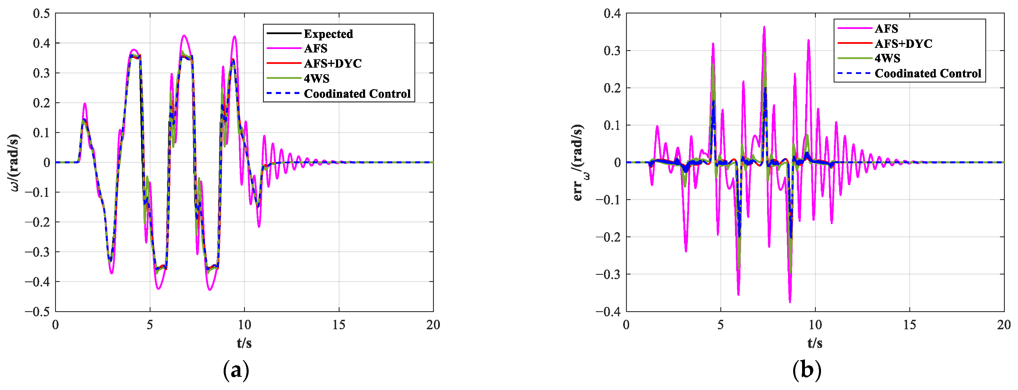
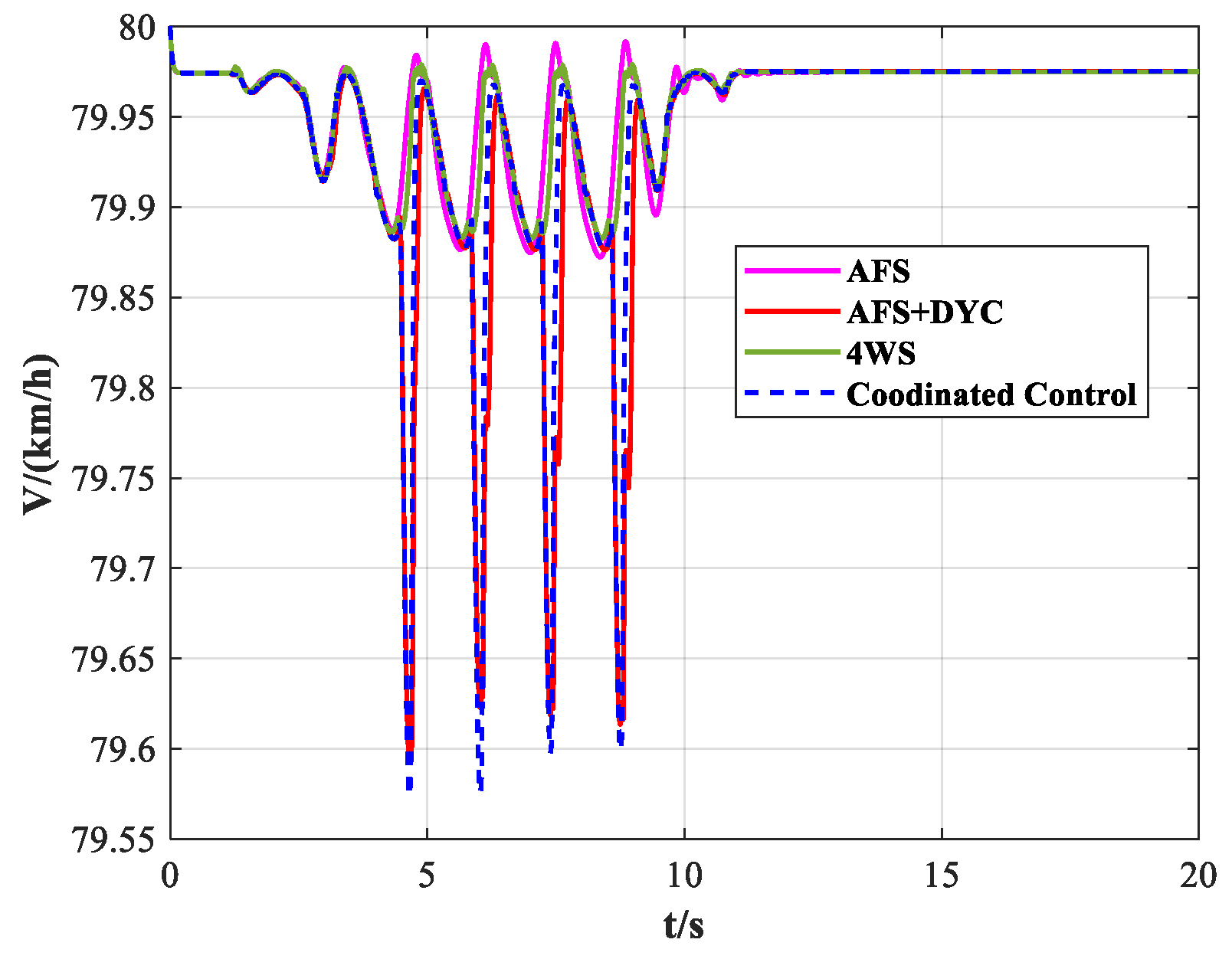
3.2.1. Slalom Test

The vehicle speed is set to 80 km/h, the road adhesion coefficient is set to 0.8, and the simulation time is set to 20 s. The proposed coordinated control strategy is verified from three aspects: trajectory tracking results, handling stability results, and economy results.

The longitudinal tracking results are presented in Figure 12. During the slalom test, the longitudinal velocity tracking based on the expert PID performs well in tracking the desired velocity, with a tracking error of less than 0.5 km/h. This meets the accuracy requirements for longitudinal tracking. Moreover, when compared with the control results of AFS, the longitudinal tracking results of AFS + DYC and coordinated control exhibit significant fluctuations and relatively reduced tracking accuracy.

The results of the lateral tracking are presented in Figure 13 and

Table 1. Comparison of path tracking errors under slalom test.

Control Strategy	Lateral Offset (m)		Heading Angle Error (Rad)
	Max	RMS	Max	RMS
AFS	0.1206	0.0439	0.0453	0.0107
AFS + DYC	0.1076	0.0453	0.0308	0.0071
4WS	0.1053	0.0435	0.0302	0.0070
Coordinated Control	0.1062	0.0445	0.0286	0.0067

. The AFS strategy, based on lateral path tracking using MPC, demonstrates good tracking performance with minimal errors, meeting the accuracy requirements. Comparing the lateral offsets and heading angle errors under different strategies, it is observed that AFS + DYC, 4WS, and coordinated control outperform AFS. Among these, 4WS exhibits the best lateral displacement tracking performance, with a maximum error of 0.1053 m and an RMS value of 0.0435 m. Coordinated control closely follows, with a maximum error of 0.1062 m and an RMS value of 0.0445 m. In terms of heading angle tracking, coordinated control performs the best, with a maximum error of 0.0286 rad and an RMS value of 0.0067 rad, followed by 4WS, with a maximum error of 0.0302 rad and an RMS value of 0.0070 rad. These results indicate that 4WS and the proposed coordinated control strategy have the best tracking performance, while AFS + DYC shows relatively poorer tracking performance but still outperforms the pure tracking control strategy of AFS. In summary, the lateral tracking results can be summarized as follows: 4WS ≈ coordinated control > AFS + DYC > AFS.

The handling stability results are presented in Figure 14 and Figure 15 and

Table 2. Comparison of handling stability errors under slalom test.

Control Strategy	Yaw Rate Error (Rad/s)		Sideslip Angle Error (Rad)
	Max	RMS	Max	RMS
AFS	0.3752	0.0878	0.0536	0.0171
AFS + DYC	0.2393	0.0306	0.0328	0.0112
4WS	0.2957	0.0433	0.0347	0.0118
Coordinated Control	0.2037	0.0258	0.0326	0.0108

. During the slalom test, AFS + DYC, 4WS, and coordinated control all exhibit better handling stability compared to the simulation results of AFS. Notably, coordinated control demonstrates the highest level of handling stability, with a maximum yaw rate error of 0.2037 rad/s and an RMS value of 0.0258 rad/s. The maximum sideslip angle error is 0.0326 rad, with an RMS value of 0.0108 rad. In summary, the handling stability results can be ranked as follows: coordinated control > AFS + DYC > 4WS > AFS.

Under the slalom test, comparing the path tracking results and handling stability results of AFS + DYC and 4WS, it can be seen that the path tracking results of 4WS are superior to those of AFS + DYC, while the handling stability results are worse. Therefore, the 4WS strategy can achieve better trajectory tracking performance than the AFS + DYC strategy but sacrifices a certain degree of handling stability accuracy. Conversely, the AFS + DYC strategy exhibits the opposite trend.

In order to take advantage of both, the coordinated controller adjusts the control weights of the drive and steering subsystems, as shown in Figure 16. When the vehicle is still in the linear region, the controller maximizes the effect of tire lateral forces, with 4WS being the primary contributor. As the vehicle gradually deviates from the linear region and tire lateral forces approach saturation, the weight of DYC increases. This explains why the coordinated controller can achieve improved trajectory tracking control while enhancing handling stability.

In this study, the simulation results are compared between the equal distribution strategy and the proposed compound distribution strategy using the system’s comprehensive efficiency and battery energy consumption as economic evaluation indicators. Figure 17 shows that under the slalom test, the system comprehensive efficiency of the proposed compound distribution strategy is superior to that of the equal distribution strategy. Additionally, the energy consumption of the battery is reduced from 240.8691 kJ to 234.4290 kJ, representing a 2.67% decrease when using the compound distribution strategy. This confirms the effectiveness of the proposed compound distribution strategy in terms of energy consumption economy.

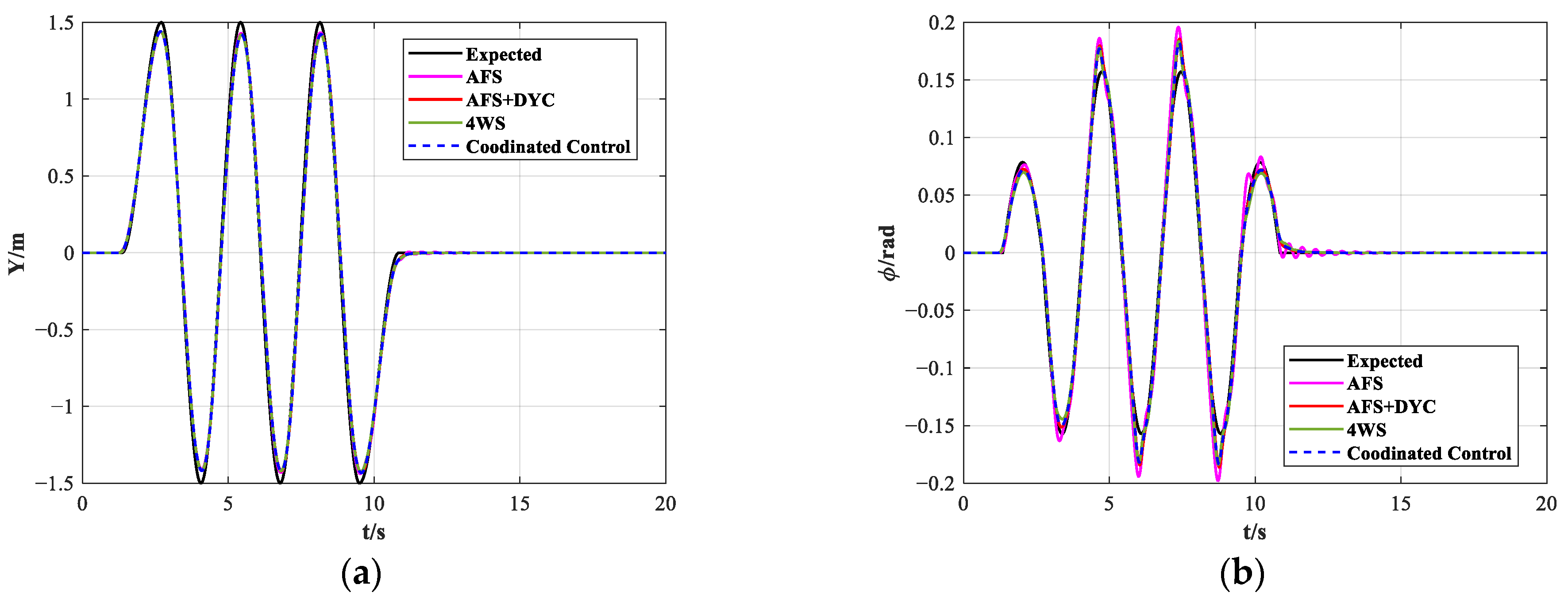
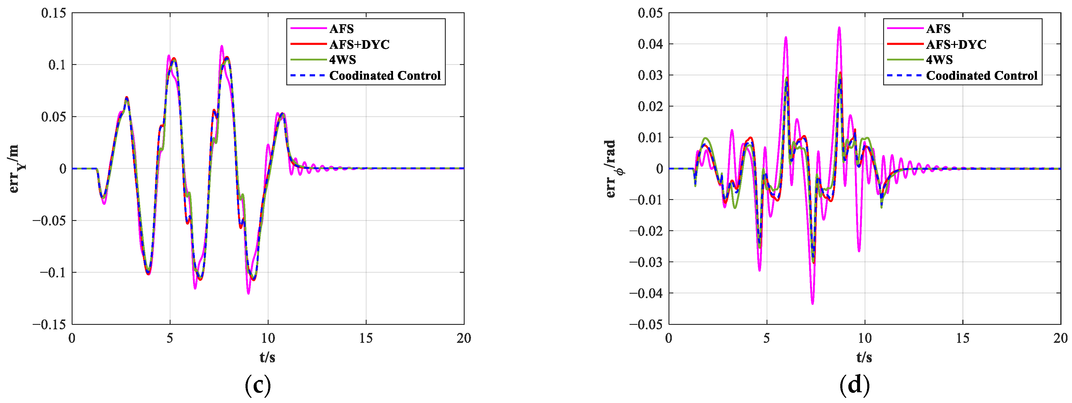
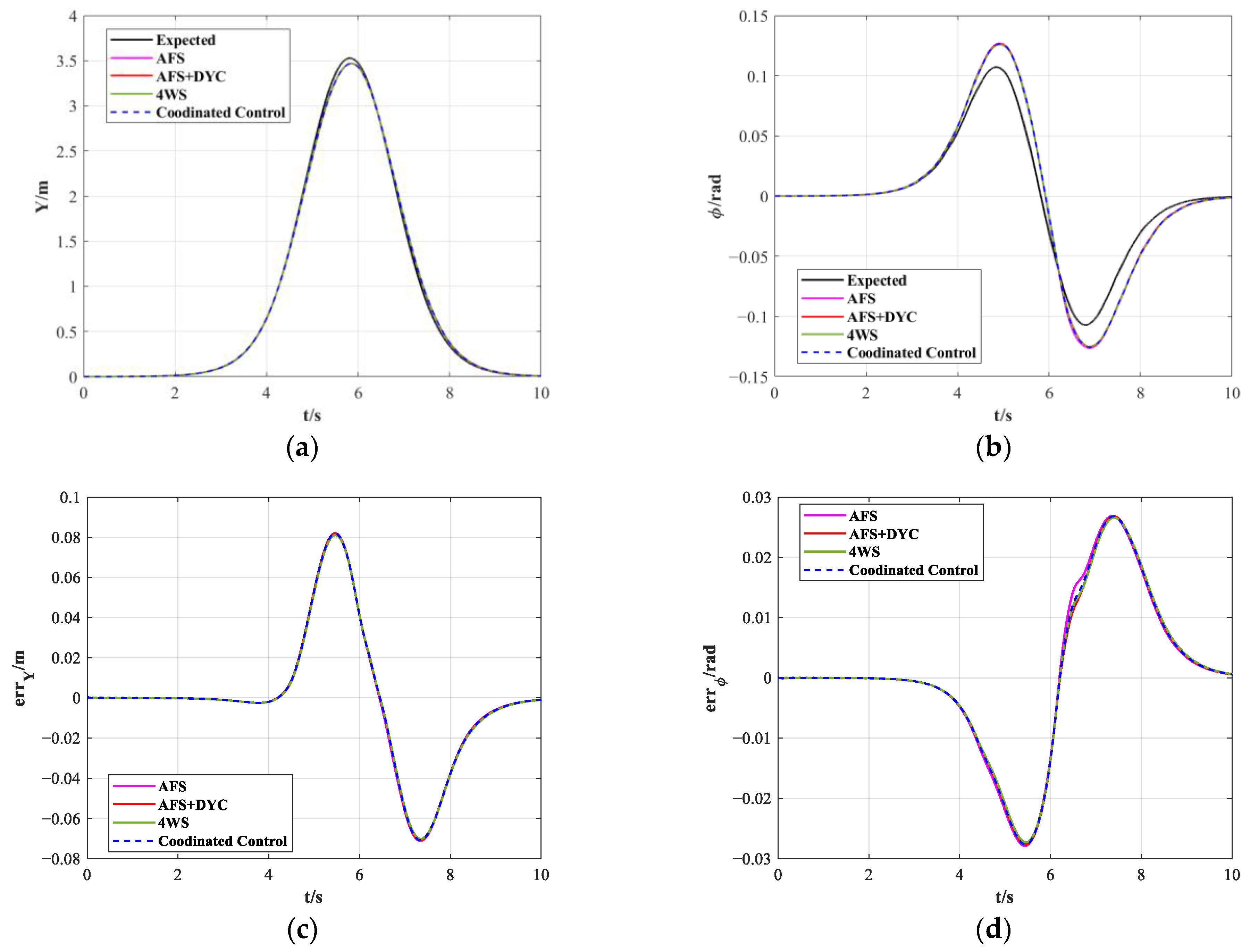
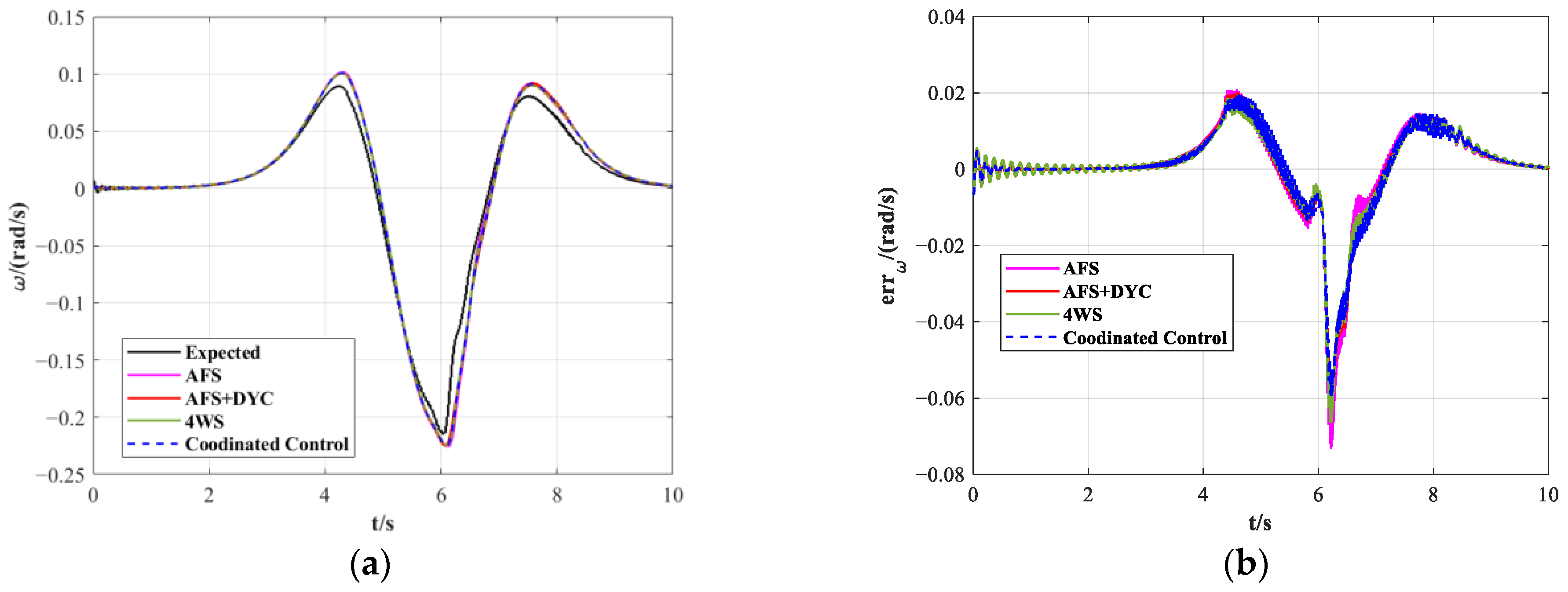
3.2.2. Double-Lane Change

The vehicle speed is set to 60 km/h, the road adhesion coefficient is set to 0.4, and the simulation time is set to 10 s. The proposed coordinated control strategy is verified from three aspects: trajectory tracking results, handling stability results, and economy results.

The longitudinal tracking results are shown in Figure 18. Under the double-lane change scenarios, longitudinal velocity tracking based on the performs well in tracking the desired velocity, with a tracking error of less than 0.2 km/h. It meets the accuracy requirements for longitudinal tracking. In addition, comparing the tracking results under different strategies, the longitudinal tracking results are basically the same.

The lateral tracking results are presented in Figure 19 and

Table 3. Comparison of path tracking errors under double-lane change.

Control Strategy	Lateral Offset (m)		Heading Angle Error (Rad)
	Max	RMS	Max	RMS
AFS	0.0821	0.0324	0.0278	0.0130
AFS + DYC	0.0819	0.0322	0.0276	0.0128
4WS	0.0811	0.0320	0.0273	0.0127
Coordinated Control	0.0814	0.0321	0.0276	0.0127

. In the double-lane change scenarios, the AFS strategy demonstrates effective lateral path tracking based on MPC, even on low-adhesion roads. When comparing the lateral offsets and heading angle errors among different strategies, it is evident that AFS + DYC, 4WS, and coordinated control outperform AFS in terms of lateral tracking results. Among these strategies, 4WS exhibits the best lateral displacement tracking and heading angle tracking effects, with a maximum lateral offset of 0.0811 m and an RMS value of 0.0320 m. The maximum heading angle error is 0.0273 rad, with an RMS value of 0.0127 rad. Coordinated control closely follows, with a maximum lateral offset of 0.0814 m and an RMS value of 0.0321 m. The maximum heading angle error is 0.0276 rad, with an RMS value of 0.0127 rad. These results indicate that 4WS demonstrates the highest tracking performance, followed by coordinated control. AFS + DYC shows relatively poorer tracking performance but still outperforms the pure tracking control strategy of AFS. In summary, the ranking of the lateral tracking results is as follows: 4WS > coordinated control > AFS + DYC > AFS.

The handling stability results are presented in Figure 20 and Figure 21, and

Table 4. Comparison of handling stability errors under double-lane change.

Control Strategy	Yaw Rate Error (Rad/s)		Sideslip Angle Error (Rad)
	Max	RMS	Max	RMS
AFS	0.3752	0.0878	0.0536	0.0171
AFS + DYC	0.2393	0.0306	0.0328	0.0112
4WS	0.2957	0.0433	0.0347	0.0118
Coordinated Control	0.2037	0.0258	0.0326	0.0108

. In the double-lane change scenarios, AFS + DYC, 4WS, and coordinated control all exhibit superior handling stability compared to the simulation results of AFS. Among these, coordinated control demonstrates the highest level of handling stability, with a maximum yaw rate error of 0.0597 rad/s and an RMS value of 0.0115 rad/s. The maximum sideslip angle error is 0.032 rad, with an RMS value of 0.014 rad. In summary, the handling stability results can be ranked as follows: coordinated control > AFS + DYC > 4WS > AFS.

In the context of double-lane change scenarios, a comparison was made between the path tracking results and handling stability results of the AFS + DYC and 4WS strategies. It was observed that the 4WS strategy outperforms in terms of path tracking, while the AFS + DYC strategy exhibits better handling stability. These findings align with the results obtained from the slalom test.

To achieve both trajectory tracking control and good handling stability, the coordinated controller adjusts the control weights, as depicted in Figure 22. A trade-off is made between the two objectives. Due to a lower road adhesion coefficient, the friction ellipse of the tires becomes smaller, leading to a higher likelihood of lateral forces reaching saturation. To address this, the coordinated controller relies more on DYC control and adjusts the longitudinal forces of the tires to enhance stability. Consequently, the lateral path tracking performance under the coordinated control strategy is slightly inferior to that of 4WS, but the handling stability surpasses other strategies.

The economic simulation results for the double-lane change scenario are presented in Figure 23. The comprehensive efficiency of the proposed compound distribution strategy is higher than that of the equal distribution strategy. Additionally, the energy consumption of the battery is 39.901 kJ under the equal distribution strategy, whereas it is reduced to 38.2123 kJ under the compound distribution strategy, resulting in a 4.23% decrease in energy consumption. These findings confirm the effectiveness of the proposed compound distribution strategy in terms of energy consumption economy.

4. Discussion

Comparing the slalom test results on a high-adhesion road and the double-lane change results on a low-adhesion road, the following conclusions can be summarized:

• The designed PID-based longitudinal velocity tracking controller and MPC-based lateral path tracking controller in this study both achieve good tracking performance, meeting the accuracy requirements of trajectory tracking control.
• When comparing the 4WS and AFS + DYC strategies, the 4WS strategy provides better path tracking performance, while the AFS + DYC strategy offers better handling stability.
• Stability and path tracking accuracy interact with each other. Improved stability leads to a decrease in path tracking accuracy, and the increase in path tracking accuracy reduces vehicle stability. The proposed coordinated control strategy maximizes the advantages of the steering and drive subsystems. By combining 4WS with DYC, it comprehensively controls stability and path tracking accuracy. This strategy can achieve better trajectory tracking control while improving the vehicle’s handling stability, realizing coordinated control with dual objectives.
• The proposed compound torque distribution strategy can enhance the vehicle’s economy while maintaining trajectory tracking performance and stability.

To further clarify the characteristics of the proposed control strategy in this study, a comparison is made with chassis coordinated control strategies proposed in References [24,25]. Both references utilized chassis coordinated control strategies that were based on extension theory and dynamically adjusted the control weights for the driving and steering subsystems. Hence, by combining the findings from these two studies, an analysis is conducted from two perspectives, as shown in

Table 5. Comparison of different control strategies.

Control Strategy	Stability Domain Division		Control Weights
	Extension Domain	Non-Domain	System	Strategy
Ref [24]	Phase diagram boundaries	Scaling factor	AFS + DYC	Correlation function
Ref [25]	Tire’s linear zone	Phase diagram boundaries	AFS + DYC	Game theory
Proposed strategy	Vehicle’s linear zone	Phase diagram boundaries	4WS + DYC	Correlation function

.

• Division of Stability Domain:

Reference [24] selected traditional phase diagram boundaries as the extension domain boundaries and expanded them to obtain non-domain boundaries using a fixed scaling factor. However, this strategy lacks a theoretical basis and cannot be adjusted according to external conditions, resulting in overly conservative extension domain boundaries and potential instability. In contrast, Reference [25] utilized the tire’s linear zone limit as the extension domain boundary and the traditional phase diagram boundary as the non-domain boundary. However, this approach cannot accurately determine the critical angle of the tire’s linear zone and cannot adaptively adjust to external environmental conditions. In this paper, we propose a strategy that defines the vehicle’s linear zone as the extension domain boundary and the traditional phase diagram boundary as the non-domain boundary. Both extension domain and non-domain boundaries can be adaptively adjusted based on the vehicle’s speed and road adhesion conditions, enabling a more accurate assessment of the vehicle’s lateral motion state.

• Adaptive Adjustment of Control Weights:

Reference [24] developed allocation coefficients for AFS and DYC control weights based on the correlation function of extension theory. In a similar vein, Reference [25] optimized the control allocation coefficients for AFS and DYC control weights using a combination of correlation functions and game theory. In contrast, this paper’s control strategy directly determines control weights for 4WS and DYC based on the correlation function. While References [24,25] focused on the control weights of the AFS system, our study takes into account the impact of ARS on vehicle lateral motion, fully utilizing the steering system’s role in handling stability. Furthermore, both Reference [24] and our strategy design control weights based on the correlation function, which is a simple, efficient, and practical approach. However, it heavily relies on the precise boundary definition of the stability domain. On the other hand, Reference [25] incorporates game theory to dynamically optimize the weights of the driving and steering systems, potentially leading to superior control outcomes. Nonetheless, this approach involves more adjustment parameters, increases computational complexity, and reduces real-time performance, posing challenges for practical engineering applications.

By considering both aspects, the control strategy proposed in this paper can dynamically adjust the boundaries of the stability domain, resulting in a more accurate assessment of the vehicle’s lateral motion state. Additionally, the allocation strategy for control weights is relatively simple and, when combined with more precise stability domain boundaries, can yield excellent control results.

5. Conclusions

This paper presents a study on the coordinated control problem of 4WID-4WIS electric vehicles, focusing on trajectory tracking performance, handling stability, and economy. Additionally, it addresses the coupling allocation issue between the driving and steering subsystems. To tackle these challenges, the paper proposes a hierarchical chassis control architecture. The expert PID algorithm is used for longitudinal velocity tracking, while the MPC algorithm is employed for lateral path tracking. To achieve optimal control of trajectory tracking performance and handling stability, a sliding mode controller is utilized to calculate the additional yaw moment. Additionally, a coordinated control strategy based on the extension dynamic stability domain is designed, where the control weights of DYC and ARS are adaptively adjusted to output the optimal control objectives. Taking into consideration the demand for energy efficiency, the optimal wheel drive torques are calculated using MPSO and QP with driving efficiency and tire adhesion ratio as control objectives. Simulation test results demonstrate that the coordinated control strategy improves trajectory tracking performance, handling stability, and economy, achieving multi-objective coordinated control of the chassis. This method has high real-time performance, simple implementation, and strong adaptability to working conditions, laying the foundation for further research on chassis-integrated control.

In future work, vehicle tests will be conducted to validate the effectiveness of the control strategy. Furthermore, the impact of vertical dynamics will be considered, and a deeper investigation into the coupling characteristics between subsystems will be carried out to achieve multi-dimensional dynamic optimization control of the chassis subsystems.

References

- He, S.W.; Fan, X.B.; Wang, Q.W.; Chen, X.B.; Zhu, S.W. Review on Torque Distribution Scheme of Four-Wheel In-Wheel Motor Electric Vehicle. Machines 2022, 10, 619. [Google Scholar] [CrossRef]
- Peng, H.; Chen, X.B. Active Safety Control of X-by-Wire Electric Vehicles: A Survey. SAE Int. J. Veh. Dyn. Stab. NVH 2022, 6, 115–133. [Google Scholar] [CrossRef]
- Zhang, L.; Zhang, Z.Q.; Wang, Z.P.; Deng, J.J.; Dorrell, D.G. Chassis Coordinated Control for Full X-by-Wire Vehicles—A Review. Chin. J. Mech. Eng. 2021, 34, 42. [Google Scholar] [CrossRef]
- Hang, P.; Chen, X.B. Towards Autonomous Driving: Review and Perspectives on Configuration and Control of Four-Wheel Independent Drive/Steering Electric Vehicles. Actuators 2021, 10, 184. [Google Scholar] [CrossRef]
- Song, P.; Tomizuka, M.; Zong, C.F. A novel integrated chassis controller for full drive-by-wire vehicles. Veh. Syst. Dyn. 2015, 53, 215–236. [Google Scholar] [CrossRef]
- Lai, F.; Huang, C.Q.; Jiang, C.Y. Comparative Study on Bifurcation and Stability Control of Vehicle Lateral Dynamics. SAE Int. J. Veh. Dyn. Stab. NVH 2022, 6, 35–52. [Google Scholar] [CrossRef]
- Peng, H.N.; Wang, W.D.; Xiang, C.L.; Li, L.; Wang, X.Y. Torque Coordinated Control of Four In-Wheel Motor Independent-Drive Vehicles With Consideration of the Safety and Economy. IEEE Trans. Veh. Technol. 2019, 68, 9604–9618. [Google Scholar] [CrossRef]
- Xu, F.X.; Liu, X.H.; Chen, W.; Zhou, C. Dynamic Switch Control of Steering Modes for Four Wheel Independent Steering Rescue Vehicle. IEEE Access 2019, 7, 135595–135605. [Google Scholar] [CrossRef]
- Zhang, B.H.; Lu, S.B.; Zhao, L.; Xiao, K.X. Fault-tolerant control based on 2D game for independent driving electric vehicle suffering actuator failures. Proc. Inst. Mech. Eng. Part D J. Automob. Eng. 2020, 234, 3011–3025. [Google Scholar] [CrossRef]
- Wang, J.N.; Gao, S.L.; Wang, K.; Wang, Y.; Wang, Q.S. Wheel torque distribution optimization of four-wheel independent-drive electric vehicle for energy efficient driving. Control Eng. Pract. 2021, 110, 104779. [Google Scholar] [CrossRef]
- Li, D.F.; Liu, A.; Pan, H.; Chen, W.T. Safe, Efficient and Socially-Compatible Decision of Automated Vehicles: A Case Study of Unsignalized Intersection Driving. Automot. Innov. 2023, 6, 281–296. [Google Scholar] [CrossRef]
- Zhang, X.; Li, J.; Ma, Z.; Chen, D.; Zhou, X. Lateral Trajectory Tracking of Self-Driving Vehicles Based on Sliding Mode and Fractional-Order Proportional-Integral-Derivative Control. Actuators 2023, 13, 7. [Google Scholar] [CrossRef]
- Liu, K.; Wen, G.; Fu, Y.; Wang, H. A Hierarchical Lane-Changing Trajectory Planning Method Based on the Least Action Principle. Actuators 2023, 13, 10. [Google Scholar] [CrossRef]
- Tong, Y.W.; Li, C.; Wang, G.; Jing, H. Integrated Path-Following and Fault-Tolerant Control for Four-Wheel Independent-Driving Electric Vehicles. Automot. Innov. 2022, 5, 311–323. [Google Scholar] [CrossRef]
- Hang, P.; Xia, X.; Chen, G.; Chen, X. Active Safety Control of Automated Electric Vehicles at Driving Limits: A Tube-Based MPC Approach. IEEE Trans. Transp. Electrif. 2022, 8, 1338–1349. [Google Scholar] [CrossRef]
- Guo, N.; Zhang, X.; Zou, Y. Real-Time Predictive Control of Path Following to Stabilize Autonomous Electric Vehicles Under Extreme Drive Conditions. Automot. Innov. 2022, 5, 453–470. [Google Scholar] [CrossRef]
- Ren, Y.; Zheng, L.; Khajepour, A. Integrated model predictive and torque vectoring control for path tracking of 4-wheel-driven autonomous vehicles. IET Intell. Transp. Syst. 2019, 13, 98–107. [Google Scholar] [CrossRef]
- Hu, C.; Wang, R.; Yan, F.; Chen, N. Output Constraint Control on Path Following of Four-Wheel Independently Actuated Autonomous Ground Vehicles. IEEE Trans. Veh. Technol. 2016, 65, 4033–4043. [Google Scholar] [CrossRef]
- Mousavinejad, E.; Han, Q.L.; Yang, F.W.; Zhu, Y.; Vlacic, L. Integrated control of ground vehicles dynamics via advanced terminal sliding mode control. Veh. Syst. Dyn. 2017, 55, 268–294. [Google Scholar] [CrossRef]
- Mirzaeinejad, H.; Mirzaei, M.; Rafatnia, S. A novel technique for optimal integration of active steering and differential braking with estimation to improve vehicle directional stability. ISA Trans. 2018, 80, 513–527. [Google Scholar] [CrossRef]
- Zhang, H.; Li, X.S.; Shi, S.M.; Liu, H.F.; Guan, R.; Liu, L. Phase Plane Analysis for Vehicle Handling and Stability. Int. J. Comput. Intell. Syst. 2011, 4, 1179–1186. [Google Scholar] [CrossRef]
- Liang, Y.; Li, Y.; Yu, Y.; Zheng, L. Integrated lateral control for 4WID/4WIS vehicle in high-speed condition considering the magnitude of steering. Veh. Syst. Dyn. 2019, 58, 1711–1735. [Google Scholar] [CrossRef]
- Tian, J.; Wang, Q.; Ding, J.; Wang, Y.Q.; Ma, Z.S. Integrated Control With DYC and DSS for 4WID Electric Vehicles. IEEE Access 2019, 7, 124077–124086. [Google Scholar] [CrossRef]
- Chen, W.W.; Liang, X.T.; Wang, Q.D.; Zhao, L.F.; Wang, X. Extension coordinated control of four wheel independent drive electric vehicles by AFS and DYC. Control Eng. Pract. 2020, 101, 104504. [Google Scholar] [CrossRef]
- Zheng, Z.C.; Zhao, X.; Wang, S.; Yu, Q.; Zhang, H.C.; Li, Z.K.; Chai, H.; Han, Q. Extension coordinated control of distributed-driven electric vehicles based on evolutionary game theory. Control Eng. Pract. 2023, 137, 105583. [Google Scholar] [CrossRef]
- Liu, R.Q.; Wei, M.X.; Zhao, W.Z. Trajectory tracking control of four wheel steering under high speed emergency obstacle avoidance. Int. J. Veh. Des. 2018, 77, 1–21. [Google Scholar] [CrossRef]
- Xu, N.; Zhou, J.F.; Li, X.Y.; Li, F. Analysis of the Effect of Inflation Pressure on Vehicle Handling and Stability under Combined Slip Conditions Based on the UniTire Model. SAE Int. J. Veh. Dyn. Stab. NVH 2021, 5, 259–277. [Google Scholar] [CrossRef]
- Yu, Z.; Wang, J. Automatic Vehicle Trajectory Tracking Control with Self-calibration of Nonlinear Tire Force Function. In Proceedings of the 2017 American Control Conference (ACC), Seattle, WA, USA, 24–26 May 2017; pp. 985–990. [Google Scholar]
- Attia, R.; Orjuela, R.; Basset, M. Combined longitudinal and lateral control for automated vehicle guidance. Veh. Syst. Dyn. 2014, 52, 261–279. [Google Scholar] [CrossRef]
- Qiao, Y.R.; Chen, X.B.; Liu, Z. Trajectory Tracking Coordinated Control of 4WID-4WIS Electric Vehicle Considering Energy Consumption Economy Based on Pose Sensors. Sensors 2023, 23, 5496. [Google Scholar] [CrossRef] [PubMed]
- Wu, X.J.; Zhou, B.; Wen, G.L.; Long, L.F.; Cui, Q.J. Intervention criterion and control research for active front steering with consideration of road adhesion. Veh. Syst. Dyn. 2018, 56, 553–578. [Google Scholar] [CrossRef]
- Wong, A.; Kasinathan, D.; Khajepour, A.; Chen, S.K.; Litkouhi, B. Integrated torque vectoring and power management framework for electric vehicles. Control Eng. Pract. 2016, 48, 22–36. [Google Scholar] [CrossRef]
- Marini, F.; Walczak, B. Particle swarm optimization (PSO). A tutorial. Chemom. Intell. Lab. Syst. 2015, 149, 153–165. [Google Scholar] [CrossRef]