Real-Time Point Recognition for Seedlings Using Kernel Density Estimators and Pyramid Histogram of Oriented Gradients

Abstract

This paper introduces a new real-time method based on a combination of kernel density estimators and pyramid histogram of oriented gradients for identifying a point of interest along the stem of seedlings suitable for stem–stake coupling, also known as the ‘clipping point’. The recognition of a clipping point is a required step for automating the stem–stake coupling task, also known as the clipping task, using the robotic system under development. At present, the completion of this task depends on the expertise of skilled individuals that perform manual clipping. The robotic stem–stake coupling system is designed to emulate human perception (in vision and cognition) for identifying the clipping points and to replicate human motor skills (in dexterity of manipulation) for attaching the clip to the stem at the identified clipping point. The system is expected to clip various types of vegetables, namely peppers, tomatoes, and cucumbers. Our proposed methodology will serve as a framework for automatic analysis and the understanding of the images of seedlings for identifying a suitable clipping point. The proposed algorithm is evaluated using real-world image data from propagation facilities and greenhouses, and the results are verified by expert farmers indicating satisfactory performance. The precise outcomes obtained through this identification method facilitate the execution of other autonomous functions essential in precision agriculture and horticulture.

1. Introduction

One of the most time-consuming and laborious tasks in facilities specializing in seedling propagation is the attachment of a clip at a specific location along the seedling stem to couple the stem to a wooden stake. This action, called stem–stake coupling or clipping, requires a human worker to bend over a wide tray containing the seedlings or to place a knee on the floor (as shown in Figure 1) and use two hands to put a plastic clip around the seedling’s main stem and the wooden stake. The clip provides support for the seedling during transportation and further growth. In greenhouses, such clips are used to force the plant to grow in the desired direction and to expedite growth and streamline harvesting. The clips are also necessary for supporting the plant’s heavy weight during growth and fruiting. The clipping task involves a significant amount of manual labor to process a large number of seedlings in a vast arena. This is a physically demanding and painstaking task. In a typical propagation facility (e.g., Roelands Plant Farms in Lambton Shores, ON, Canada), approximately 25 million seedlings are germinated annually. Each seedling is manually clipped before shipping. The sheer volume of seedlings processed each year underscores the necessity and advantages of developing a robotic solution for automated clipping. Such a solution would lead to tangible improvements in process efficiency, productivity, and product quality. Additionally, it would significantly reduce the labor costs associated with the clipping task and prevent work-related injuries, such as back injuries, strains, and sprains resulting from performing awkward body positions for an extend period of time.

A robotic clipping solution requires two main components: a machine vision unit that analyzes an image of a seedling and identifies the clipping point and a mechatronic unit that performs the act of clipping. The focus of this paper is on the machine vision unit that replicates human visual and cognitive functionalities to understand an image and identify a suitable clipping point along the seedling’s main stem for different types of vegetables, namely peppers, tomatoes, and cucumbers. In recent years, machine vision and various visual processing algorithms have seen significant advancements in agriculture-related applications [1]. These applications span a wide range of tasks, including spraying fertilizers and pesticides [2], plant detection and harvesting [3], grafting, irrigation, automatic grading [4], plant disease detection [5], ripe fruit identification [6], crop-weed classification [7], and cutting or pruning [8].

Real-time point recognition refers to the ability of a system or algorithm to identify and locate a specific point or key points in an image or video stream in real time. Real-time recognition of a suitable clipping point is a challenging problem in image processing as it requires the modeling of the human’s cognitive processes and past experiences. We extensively reviewed various approaches in the literature that could potentially address this problem. Each approach has its strengths and limitations when applied to this specific task. Some studies, such as those examining multi-feature patch-based segmentation [9], adaptive spectral–spatial gradient sparse regularization [10], the adaptive snake algorithm model [11], kernel-based algorithms based on the adaptive Kalman filter [12], and the SIFT feature descriptor with hybrid optimization algorithms [13], offer rigorous mathematical analysis and quantitative measures of computer vision. These algorithms encounter significant challenges in dealing with occlusions caused by leaves and neighboring seedlings, varying lighting conditions, and different backgrounds in various greenhouse settings. Consequently, adapting vision algorithms for real-time and reliable results in such diverse conditions becomes crucial. Alternatively, end-to-end deep learning models [14,15] are particularly effective in scenarios where the input data can be directly mapped to the desired output without the need for extensive pre-processing or feature engineering. These models require hundreds, if not thousands, of labeled images for training the network for each seedling type, leading to substantial processing times, also known as latency or inference time [16]. These challenges render the abovementioned algorithms less suitable and less robust for our specific application. Recently, feature-based methods employing machine learning techniques and complex optimization frameworks [17,18] have shown promise in modeling processes that rely on heuristic knowledge and human experience. However, feature-based methods often require manually engineered features which limit their performance to specific conditions or scenarios for which these features were designed. It can be challenging to create features that adequately represent the underlying patterns in all possible conditions. This process becomes increasingly difficult as the complexity and variability of conditions grow considering seedling types, sizes, shapes, and patterns. In addition, complex optimization frameworks can be computationally intensive and may require substantial resources, making them impractical for real-time applications or situations with limited computational power [19].

To address these challenges, we take advantage of a hybrid approach based on analytical image processing and data-driven learning algorithms. By integrating traditional and modern approaches, we aim to overcome the problems associated with varying lighting and environmental conditions and adapting to different types of seedlings. The analytical part of our proposed method calculates feature descriptors based on point density variation, kernel density estimation, and pyramid histogram of oriented gradients. The data-driven learning part of our algorithm uses Extreme Gradient Boosting to select the most suitable clipping point using the feature descriptors obtained in the analytical part. We applied the algorithm to one hundred images of real seedlings from “Roelands Plant Farms” and expert farmers reviewed the results to evaluate the performance and accuracy of the proposed method. We equipped a robotic arm with a proprietary clipping device and a stereo camera to assess the performance of our methodology. The accurate results derived from this identification method open up the possibility of implementing other autonomous functionalities required in precision agriculture.

The contributions of this work are as follows:

-

Introducing a real-time hybrid method to find the most suitable clipping point on seedlings.

-

Comparing proposed method with deep learning based methods.

-

Real-time evaluation of the results using a large number of in situ images.

-

Experimental studies using a robotic system to validate the performance of the proposed method

The organization of the paper is as follows: Section 2 describes the materials and methods. Section 3 contains the evaluation strategy and dataset. Section 4 represents the results, and Section 5 summarizes and concludes the paper.

2. Materials and Methods

2.1. Suitable Clipping Point

The selection of a clipping point for each seedling varies based on factors such as type, age, height, dimensions of inter-nodes and petioles, size and arrangement of leaves, and the number of nodes. Farmers put the clip on the highest point, higher than the uppermost node on the main stem. However, if the length of the main stem is too short between the two nodes or the seedling height surpasses that of the stake, the clipping point is selected below the highest node. The leaves around the highest node are often dense and some parts of the main stem are behind the leaves. The thickness and shape of the stem and petioles are the same, especially in the top parts of a seedling. Thus, recognizing the main stem from the petioles using machine vision is not an easy task. The recognition process also depends on the shape and type of seedlings. The spatial distance between the stake and stem and the accessibility of the point through the leaves must be taken into consideration, which further complicates the selection of a correct point for clipping. The selection of the clipping point is not a straight forward task but rather a cognitive process that relies heavily on heuristic information. Figure 2 shows some seedlings and the preferred clipping points that expert farmers have validated. As seen, the locations of the selected clipping points do not follow a specific pattern that can be algorithmized.

2.2. General Concept

The recognition of a suitable clipping point using the combination of a kernel density estimator (KDE) and pyramid histogram of oriented gradients (PHOG) is a promising approach in computer vision and image processing. The KDE is a non-parametric way to estimate the probability density function of a random variable, while PHOG is a feature descriptor that captures the local shape information in an image. 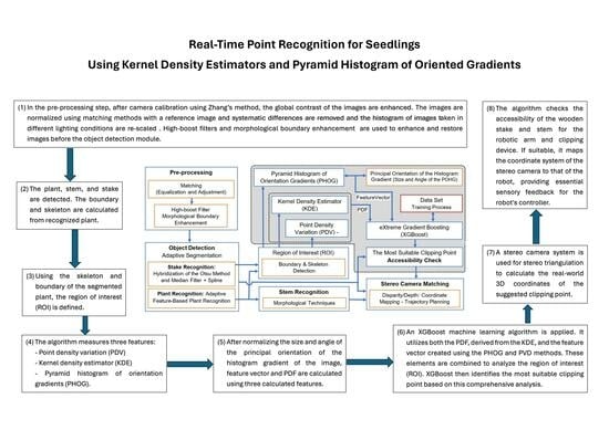Figure 3 shows the schematic of our proposed method using images taken with a stereo camera. In the pre-processing step, after camera calibration using Zhang’s method [20], the global contrast of the image is enhanced using the histogram equalization. To normalize all images for different lighting conditions, the cumulative distribution function matching method is used to balance the target images with a reference image by removing systematic differences or re-scaling the histogram of images taken in different lighting conditions [21]. High-boost filters and morphological boundary enhancement [22] are used to enhance and restore images before the object detection module. In the next step, the plant, stem, and stake are detected. We then use the boundary and skeleton of the segmented plant to find the region of interest (ROI), limit the searching area, avoid unwanted points, and accelerate the process.

After the region of interest is selected, the point density variation (PDV) measures the disparity in each area relative to the color intensity of the plant. Using PDV allows us to extend the characteristics of each area of the image to the adjacent areas. As a result, the algorithm not only focuses on specific areas of the image, but it considers the characteristics of other pixels around the area. It improves the capabilities of the algorithm to determine some areas of the image with the same pattern but with different environments around them.

In the next step, a KDE is applied to estimate the probability density function (PDF) of key point locations. This process aids in understanding the spatial distribution of key points across the image. The KDE works by smoothing raw data to estimate the population density of such finite data samples. In image processing, the KDE is particularly useful for estimating the underlying continuous distribution of data, whether it be pixel intensities or feature values. The resulting PDF provides a representation of how these values are distributed throughout the image.

Next, we construct a feature vector using the PHOG method. This method offers a rich representation by capturing local texture and shape information within the image. It achieves this by constructing histograms of gradient orientations at varying scales and positions, arranged in a pyramid-like structure. This approach captures both local and global image characteristics.

Following this, the XGBoost machine learning algorithm is applied. It utilizes both the PDF, derived from the KDE, and the feature vector created using the PHOG and PVD methods. These elements are combined to analyze the region of interest (ROI). XGBoost then identifies the most suitable clipping point based on this comprehensive analysis.

A stereo camera system is used for stereo triangulation to calculate the real-world 3D coordinates of the suggested clipping point. In the last step, the algorithm checks the accessibility of the wooden stake and stem for the robotic arm and clipping device. If suitable, it maps the coordinate system of the stereo camera to that of the robot, providing essential sensory feedback for the robot’s controller.

2.2.1. Plant, Stem, and Stake Detection

The quality of the plant recognition is crucial for having accepted results in subsequent steps. After an exhaustive review of existing automatic segmentation algorithms, which included both classic image processing and deep learning approaches, we assessed the advantages and disadvantages of these methods. Consequently, we opted for an adaptive feature-based plant segmentation algorithm [23] as it provides the required accuracy for effective plant detection. This method is powerful since it can deal with various seedlings with different lighting conditions and complex backgrounds. Noise is removed from the segmented plant using morphological filtering techniques [24] after plant recognition. We used a combination of morphological techniques, such as hit-and-miss, thinning-and-thickening, convex hull, and morphological gradient to eliminate the leaves from the image [25]. The effectiveness of morphological operations depends on the specific characteristics of the image and the nature of the problem we are trying to solve. By choosing the right structuring element, morphological processing may remove special parts of the image based on the size and shape of these parts. In order to identify parts of the stem that are hidden behind the leaf or wrongly removed from the image when using the mathematical morphology operators, a fifth-degree polynomial spline was chosen to estimate some hidden parts of the stem. The main premise of using this technique is that the stem has a smooth shape with no sudden changes in the shape or its angle. A spline matching algorithm and hybridization of the Otsu method and median filter detects the wooden stake [26]. The wooden stake is almost vertically straight. Thus, hidden and covered parts of the stake can be detected using simple partial spline matching. Given that the stereo camera captures images from varying distances, images are resized and cropped to mitigate the effects of distance variation. The distance of the stem is calculated from the stereo matching algorithm [27]. The size ratio k is computed as follows:

$$k=\frac{\delta D_n}{Bf}$$

(1)

where $\delta$ represents the disparity, $D_n$ is the normal distance, B is the baseline distance between the cameras, and f is the focal length of the stereo camera.

2.2.2. Region of Interest

To avoid unwanted points and accelerate the process of finding the most suitable clipping point, the proposed real-time point recognition method uses the boundary and skeleton of the seedling to find the region of interest (ROI) and limit the search area. The borders of the ROI are computed as follows:

$${\overline{S}}_i-\frac{{\sum }_{i=1}^n(P_r\left(i\right)-S\left(i\right))}{(n-{\varphi }_r)}<P_i<{\overline{S}}_i+\frac{{\sum }_{i=1}^n(P_l\left(i\right)-S\left(i\right))}{(n-{\varphi }_l)}$$

(2)

and

$${\overline{S}}_j-\frac{{\sum }_{j=1}^m(P_t\left(j\right)-S\left(j\right))}{(m-{\varphi }_t)}<P_j<{\overline{S}}_j$$

(3)

where ${\overline{S}}_i$ and ${\overline{S}}_j$ are the mean values of the skeleton in the x and y directions, respectively, for all non-null pixels; $P_r$, $P_l$, and $P_t$ are, respectively, the right, left, and top values of the seedling boundaries for non-null values; $S\left(i\right)$ and $S\left(j\right)$ are the values of the skeleton in pixel $(i,j)$; and ${\varphi }_r$, ${\varphi }_l$, and ${\varphi }_t$ are the number of null values for the right, left, and top of the boundary of the plant, respectively.

2.2.3. Point Density Variation

The point density variation illustrates the disparity in color intensity across a map [28]. For each color channel i, a Gaussian mixture model represents the distribution as follows:

$$P_i\left(x\right)=\sum _{k=1}^K{\pi }_{i_k}{N}_i\left(x\right|{\mu }_{i_k},{\Sigma }_{i_k})$$

(4)

where ${\pi }_{i_k}$ are the mixing coefficients satisfying

$$\sum _{k=1}^K{\pi }_{i_k}=1,{\pi }_{i_k}\ge 0$$

(5)

The $P_i\left(x\right)$ is the combined Gaussian distribution of intensities for color channel i, in that $N\left(x\right|{\mu }_{i_k},{\Sigma }_{i_k})$ is the Gaussian density with mean ${\mu }_{i_k}$ and covariance ${\Sigma }_{i_k}$. Assuming diagonal covariance matrices of the form ${\Sigma }_i={\sigma }_i^2$ [29], the Gaussian model for each color channel simplifies to

$$P_i\left(x\right)=\frac{1}{{\left(2\pi {\sigma }_i^2\right)}^{\frac{1}{2}}}{e}^{-\frac{\left|\right|x_k-{\mu }_i{\left|\right|}^2}{2{\sigma }_i^2}}$$

(6)

where ${\mu }_i$ and ${\Sigma }_i$ are the mean and covariance values, respectively.

We applied this Gaussian model to each color channel of the segmented image. The point density variation of the seedling is represented by combining these Gaussian distributions, weighted by their respective mixing coefficients.

2.2.4. Kernel Density Estimator

In most computer vision and pattern recognition applications, feature spaces are complex and often contain noise, making them difficult to describe effectively using common parametric models. Instead, non-parametric density estimation techniques are widely used to analyze arbitrarily structured feature spaces [30]. The kernel density estimator (KDE), as a non-parametric density estimation technique, calculates the feature density in a neighborhood around those features. The density function is estimated by summing kernel functions (typically Gaussians) centered at the data points [31].

The comparison between histogram and kernel density estimation shows that a bandwidth associated with the kernel function controls the smoothness of the estimated densities. More data points allow for a narrower bandwidth, leading to a more accurate density estimate. The kernel density estimator distributes the known population quantity for each point across the location of random non-parametric variables [32]. Consequently, point density variation estimates the density of stem intensity, making kernel density estimation a fundamental data smoothing technique that makes inferences about the population from a finite data sample [33]. Assuming $X_1,X_2,\dots ,X_n$ are independent and identically distributed points that have a univariate distribution with an unknown density at any given point x, the kernel density estimator is defined as

$$\overline{f}\left(x\right)=\frac{1}{n}\sum _{i=1}^h{K}_h(x-x_i)=\frac{1}{nh}\sum _{i=1}^{h}K\left(\frac{x-x_i}{h}\right)$$

(7)

where K is the kernel, $h>0$ is a smoothing parameter called the bandwidth, and $K_h\left(x\right)=\frac{1}{h}\times K\left(\frac{x}{h}\right)$ is the scaled kernel. As a rule of thumb [34], if the Gaussian basis function is used to approximate univariate data, the optimal choice for the bandwidth is

$$h=0.9\min (\tilde{\sigma },\frac{IQR}{1.34})n^{-\frac{1}{n}}$$

(8)

where $\tilde{\sigma }$ is the approximate standard deviation and $IQR$ is the interquartile range.

2.2.5. Pyramid Histogram of Oriented Gradients

The pyramid histogram of oriented gradients (PHOG) is a feature descriptor used in computer vision for image analysis and object recognition [35]. It was introduced as an extension of histogram of oriented gradients (HOG) to capture both local and global information about the shape and structure of objects in an image. HOG represents a signature of the features of spatial regions [36] and is particularly useful when dealing with images that contain objects at different scales. PHOG divides an image into small cells and computes HOG within each cell. These histograms provide a representation of the local texture and edge information. PHOG extends HOG by incorporating a pyramid structure. Instead of analyzing the entire image at a single scale, PHOG divides the image into multiple scales or levels. This helps in capturing information at different resolutions, allowing the descriptor to be more robust to variations in object size and scale. At each level of the pyramid, HOG features are computed for local image regions (cells). The features are then concatenated to form a representation for that level. Additionally, these level-specific representations are combined across the pyramid to capture global information. For computing the HOG of each cell, we used the first quarter of the cell to compute the histogram gradient in sixteen directions. We considered all different directions and the number of pixels within each direction. These steps were repeated for other quarters. The resulting orientation histograms were concatenated to create a long histogram gradient (LHG). Figure 4 shows the main steps of computing the HOG.

To make the descriptor robust to changes in illumination and contrast, normalization is often applied. The largest gradient direction was selected as the principal orientation. We normalized the principal orientation of all histogram gradients of the cells. Normalizing the histogram diminishes the effect of scaling and ignores the magnitude of the gradient. The rotation ignores the effect of different orientations. We used (10) and (11) to calculate the size and angle of the principle of the LHG:

$$\theta =ta{n}^{-1}(\frac{\partial I}{\partial y}{|}_{max}/\frac{\partial I}{\partial x}{|}_{max})$$

(9)

$$d=\sqrt{{(\frac{\partial I}{\partial y}{|}_{max})}^2+{(\frac{\partial I}{\partial x}{|}_{max})}^2}$$

(10)

where $\frac{\partial I}{\partial x}$ is the rate of the change of the LHG in x direction and $\frac{\partial I}{\partial y}$ is the rate of the change of the LHG in y direction. This involves dividing the feature vectors by a local or global measure of their magnitude. The final PHOG descriptor was formed by concatenating the feature vectors from different levels of the pyramid. This results in a comprehensive representation of the image structure at multiple scales.

2.2.6. Extreme Gradient Boosting

Extreme Gradient Boosting (XGBoost) is primarily designed for supervised learning tasks. It is well equipped to address non-linear relationships between input features and target variables [37] and can capture intricate patterns and interactions within high-dimensional feature spaces [38]. XGBoost belongs to the ensemble learning category, specifically to the gradient boosting framework. Ensemble learning involves combining the predictions of multiple learners to create a strong learner. Gradient boosting is a technique that builds a series of models sequentially, with each new model attempting to correct the errors of the combined ensemble of models built so far. This is achieved by constructing a collection of decision trees, where each tree can represent various facets of the nonlinear relationships present in the data. The algorithm works by minimizing the cumulative loss over the entire ensemble of models, where each new model is added in a way that reduces the overall error. XGBoost is known for its efficiency and scalability, making it suitable for a wide range of machine learning tasks.

To reduce redundant information in the hyperspectral data, feature selection based on the importance of boosting was used. The implementation of model development was programmed using the Scikit-learn, XGboost, and LightGBM packages in Python 3.9 [39].

2.2.7. Overall Approach

Real-time point recognition using kernel density estimators and the pyramid histogram of oriented gradients (KDE-PHOG) algorithm follows multiple steps to find the clipping point. In this section, we briefly describe these steps using an example. In Figure 5, the plant, stem, and stake are detected following camera calibration and pre-processing. This detection uses adaptive feature-based plant segmentation, morphological techniques, and a hybrid approach combining the Otsu method and a median filter. Subsequently, the plant’s boundary and skeleton are obtained. The region of interest (ROI) is then defined based on these boundary and skeleton features of the plant.

We used PHOG to select multiple cells with different scales and levels in a pyramid structure to capture information at different resolutions. Figure 6 shows samples of the cells and histogram of PDV, the feature vector of the KDE, and normalized PHOG. It is clear that the PDF of the cell that contains the suitable clipping point is unique and different from the other cells, and XGBoost can recognize such a cell.

In the subsequent step, the ideal point for clipping is identified within the selected cell scene. This selection takes into account the presence of both the stake and the stem in that specific area as well as the distance between them. Additionally, the algorithm checks for a corresponding point on the stake near the selected clipping point. If such a point is accessible, the KDE-PHOG method is utilized to calculate the distance and depth of the point using images from a stereo camera. In the final step, the real coordinates of the clipping point are transmitted to the robotic arm, which then positions the clipping device at the specified point. Figure 7 illustrates these steps.

3. Evaluation Strategy and Datasets

To evaluate the precision of the proposed algorithm in identifying suitable clipping points, we conducted a comparative analysis against three other automatic techniques, including deep learning approaches based on Convolutional Neural Networks (CNNs).

Table 1. A brief description of methods: Faster R-CNN, Faster R-CNN and YOLOv8.

Name	Description
Faster R-CNN	Faster R-CNN has set new standards in object detection by seamlessly integrating the region proposal mechanism into the overall architecture. It provides a balance of high accuracy and efficiency, establishing itself as a fundamental model in the field of computer vision for tasks that demand accurate object localization and classification. It is primarily designed for instance segmentation, which involves identifying and delineating individual objects in an image [40].
RetinaNet	RetinaNet is an effective one-stage object detection model that employs focal loss to handle the imbalance between positive and negative samples in training. Its primary focus lies in predicting both bounding boxes and class probabilities for objects present in an image [41]. RetinaNet is adapted to predict the coordinates of points by including specific output layers.
YOLOv8	As a form of instance segmentation, YOLO combines image processing and deep learning techniques to achieve real-time object detection in both images and videos [42]. YOLOv8 can be adapted for point recognition with some modifications and by adding an extension [43].

provides a brief description of these three methods.

To compare our proposed method with others, we calculated the mean Average Precision (mAP) to evaluate the precision of clipping point detection.

Average Precision (AP) is computed by calculating the area under the precision–recall curve. It shows the relationship between two important evaluation metrics: precision (how many selected items are relevant) and recall (how many relevant items are selected). Recall is defined as follows:

$$Recall=\frac{TP}{TP+FN}$$

(11)

and precision is defined as:

$$Precision=\frac{TP}{TP+FP}$$

(12)

where $TP$ represents number of correctly detected points, $FP$ is the number of miss-detection points, and $FN$ is the number of false alarms. Mean Average Precision, $mAP$, is defined as:

$$mPA={\int }_0^{1}P\left(R\right).PdR$$

(13)

where P is precision, R is recall, and $mPA$ measures the performance of the detector. In the case of a single class, the mean Average Precision ($mAP$) is equivalent to the Average Precision ($AP$) for that class, and it can be used as a metric to standardize performance measurement. $AP$ represents the area under the precision–recall curve, and the higher the $AP$ value is, the better the detection accuracy is.

Our dataset contained real images of five different seedling types, including Beit Alpha cucumber, tomato, chili pepper, bell pepper, and national pickling cucumber. The images had different resolutions and included multi-scale seedlings with different lighting conditions and backgrounds. We utilized a dataset of 500 sample images paired with the corresponding ground truth images to train the machine learning unit. We also used approximately 1000 sample images along with ground truth images for evaluating deep learning methods. The images were acquired from seedlings that were generously supplied by Roelands Plant Farms Inc., the industrial collaborator in this venture.

4. Results and Discussion

We applied our proposed method to five types of seedlings for finding the correct position of the clipping points. These plants are real seedlings from “Roelands Plant Farms” in the stage of clipping task. We evaluated the accuracy of the results comparing the algorithm-selected points with those of the expert farmers. Each category contained 100 images of one type of seedling.

Table 2. Mean Average Precision (mAP) of selected clipping points using KDE-PHOG method for each seedling in different lighting conditions.

	Natural Light Intensity			Artificial
Seedling	Low	Medium	High	Light (LED)	Average
Tomato	83%	90%	87%	88%	87%
Bell Pepper	91%	96%	94%	95%	94%
Chili Pepper	88%	94%	89%	93%	91%
National Pickling Cucumber	81%	88%	84%	87%	85%
Beit Alpha Cucumber	82%	91%	86%	87%	87%
				Standard Deviation	3.487
				Total Average	89%

shows the mAP for each type of seedling in different lighting conditions.

Figure 8 shows the most suitable stem-stake coupling point suggested by KDE-PHOG method to four different seedlings from different lighting conditions and backgrounds. The output of the our suggested method is three parameters. D that is the distance of the camera and suggested clipping point, and Δθ_X and Δθ_Y which are the yaw and pitch correction angle factors. After rotating the robot in yaw and pitch direction with the angle of −Δθ_X and −Δθ_Y, If the robot moves in this direction as much as D, the center of the clipping device will be in the suggested clipping point in the real coordinate of the robot.

After training the deep learning algorithms, we also calculated the mAP obtained using Faster R-CNN, Retina Net, and YOLOv8 for the same set of images.

Table 3. Comparison of mean Average Precision (mAP) of KDE-PHOG and deep learning approaches in selecting the clipping point.

Seedling	Faster R-CNN	RetinaNet	YOLOv8	KDE-PHOG
Tomato	75%	78%	85%	87%
Bell Pepper	80%	83%	90%	94%
Chili Pepper	81%	85%	82%	91%
National Pickling Cucumber	74%	82%	84%	85%
Beit Alpha Cucumber	71%	78%	80%	87%
Standard Deviation	3.763	2.786	3.371	3.249
Average	76%	81%	84%	89%

shows the mAP for the selected clipping points for each type of seedling using deep learning approaches and compares them with our proposed algorithm.

In real-time applications such as ours and other scenarios where a quick response is required, latency, or computational time, is a critical factor. To compare the computational time of the proposed method and deep learning approaches, we estimated the average and maximum time of finding a clipping point for 500 images. We used the Ryzen7-7730U processor with 16 GB RAM. All codes were ruining on Jupiter notebook (ipykernel:python 3.12.1, TensorFlow 1.15.7, Keras 3.0.2, scikit-learn 1.3.2).

Table 4. Average and maximum computational time for a complete cycle of finding the clipping point.

Computational Time (ms)	Faster R-CNN	RetinaNet	YOLOv8	KDE-PHOG
Average	163	145	92	124
Maximum	208	164	116	156

shows the computational time required for each approach. Average computational time using KDE-PHOG is 124 ms. It means that the process of finding the clipping point is fast and occurs in real time.

The results in the table show that among deep learning approaches, YOLOv8 has a better performance and it even runs slightly faster than our proposed algorithm. However, considering the mPA of all approaches, it is clear that the proposed KDE-PHOG method has the best overall performance.

As seen, all approaches find the clipping point of the bell pepper more accurately. The leaves of both types of cucumbers are big and access to the stem on top of the cucumber seedlings is difficult. So, the mAP of cucumbers is less than other seedlings in all approaches.

In some cases, the stem or stake, or both, could not be accessed—for example, when hidden behind leaves or when the distance between the stem and stake was too great. In such scenarios, the algorithm was unable to suggest a suitable clipping point. As illustrated in Figure 9, for Samples A and B, the algorithm successfully suggests a suitable clipping point. However, for Sample C, it identifies a suitable but unreachable clipping point due to the excessive distance between the stake and stem. For Sample D, neither the stem nor the stake are accessible. A potential solution in these instances is to capture additional images from various angles, or even from the opposite side of the seedling. If the KDE-PHOG algorithm cannot locate the clipping point, the robotic arm has the ability to rotate the clipping device and the stereo camera around the seedling to acquire a new image and identify the clipping point from a different perspective. This approach mirrors the manual methods used by farmers. By implementing this strategy, the mAP of the method is projected to exceed 89 percent.

We designed, built, and installed a clipping device to work alongside our vision system for autonomous clipping. This device was mounted on a general-purpose robotic arm, specifically a KUKA LWR IV. The clipping mechanism operates by curling a thin wire as it attaches the clip to the plant. The clipping device incorporates an optimized stereo camera (Megapixel/USB5000W02M) to capture images of the plants and sends them to the vision algorithm. When the KDE-PHOG algorithm identifies the most suitable clipping point, the robotic arm locates the clipping device near this point to performs the clipping action. Figure 10 displays examples of seedlings with clips attached at the points identified using the KDE-PHOG algorithm. The film “manuscript-supplementary.mp4” shows the operation of an automatic clipping device with a stereo camera on it that are installed on a KUKA LWR IV robot. KDE-PHOG method recognizes the most suitable clipping point and it sends control signals to the robot to guide the robot to the suggested point. The envisioned final automated clipping system will comprise several specialized robotic arms, each equipped with a similar clipping device.

5. Conclusions

This paper introduced a novel approach in machine vision to determine a specific point on the real seedlings in the propagation facilities using the images of a stereo camera. This point is a point on the seedling stem that is suitable for placing a clamp around the stem and fork to provide more support to the seedling during growth or transportation. The proposed vision algorithm is a part of a new robotic stem–stake coupling system under development, which recognizes the suitable point for putting the clip around the stem and stake and puts the clip in the recognized point automatically using robotic arms. Identifying an appropriate clipping point in real-time is challenging due to the complexities involved in mimicking human cognitive processes and incorporating past experiences into the decision-making process. Our proposed approach combines analytical image processing methods with data-driven learning algorithms, setting it apart from deep learning methods. Evaluation of the algorithm was conducted using real seedling images of peppers, tomatoes, and cucumbers. It was shown that our proposed approach resulted in better mPA compared to other methods and an overall best performance. We concluded that the medium natural lighting intensity yielded the best overall results, while bell pepper exhibited the highest mAP, although finding the clipping point on the national pickling cucumber proved more challenging.

To enhance the effectiveness of our system, we implemented a strategy to capture additional images from different angles to reach an mAP of more than 89 percent. This approach emulates the human approach in finding the clipping point. Expert farmers verified the identified clipping points, serving as a valuable ground truth for evaluation.

While the algorithm demonstrates satisfactory performance, there are still some limitations that will be addressed in future studies. Stem recognition can be challenging when leaves cover a significant portion of the stem or when the stem’s pattern and color resemble those of the leaves behind it. To overcome this, employing multiple labeled images to train an Artificial Neural Network or using rational laws such as the continuity of the stem can be explored. Additionally, obtaining multiple images from different angles around the seedlings can be effective to deal with significant occlusions. In our current study, we focused on XGBoost to address non-linear relationships between input features and target variables. we recognize the potential of other deep-learning-based approaches to improve the quality of the results, which will be the focus of our future studies. As a real-time process, optimizing the algorithm’s speed is imperative. Further optimization of the codes for faster throughput can be achieved, and the use of a GPU or optimized hardware will be explored to increase the speed of the process. As we progress towards autonomous seedling clipping, our ongoing research aims to address the limitations, explore learning-based approaches, and optimize the algorithm for enhanced real-time performance.