Grey-Box Modeling and Decoupling Control of a Lab Setup of the Quadruple-Tank System

Abstract

The quadruple-tank system (QTS) is a popular educational resource in universities for studying multivariable control systems. It enables the analysis of the interaction between variables and the limitations imposed by multivariable non-minimum phase zeros, as well as the evaluation of new multivariable control methodologies. The works utilizing this system present a theoretical model that may be too idealistic and based on erroneous assumptions in real-world implementations, such as the linear behavior of the actuators. In other cases, an identified linear model is directly provided. This study outlines the practical grey-box modeling procedure conducted for the QTS at the University of Cordoba and provides guidance for its implementation. A configurable nonlinear model was developed and controlled in a closed loop using different controllers. Specifically, decentralized control, static decoupling control, and simplified decoupling control were compared. The simulation designs were experimentally validated with high accuracy, demonstrating that the conclusions reached with the developed model can be extrapolated to the real system. The comparison of these three control designs illustrates the advantages and disadvantages of decoupling in certain situations, especially in the presence of non-minimum phase zeros.

1. Introduction

Industrial processes are often multivariable and exhibit nonlinear behavior [1]. The interactions between components, variables to be controlled, and manipulated variables can increase the complexity of a nonlinear system. Due to the characteristics of nonlinearity, time variation, and cross-coupling between variables, classical control methods developed for single-variable systems may lead to inefficient results when they are applied to multivariable processes [2]. Additionally, the design of a multivariable process control system must consider the possible presence, location, and direction of multivariable zeros, as they can affect system stability. The design of control systems is generally based on a process model in an iterative procedure to save time and money. It is important to maintain a clear and logical flow of information with causal connections between statements. Although closed-loop control systems are less sensitive to process modeling errors, obtaining a proper model is crucial for designing a good controller. This is especially true for multivariable processes, which present greater control difficulties that the model should reflect.

Industrial process modeling has traditionally been based on white-box modeling or black-box identification. White-box modeling involves building a model using scientific relationships that fully describe the process. On the other hand, black-box identification employs a parametric model that fits the measured process data obtained experimentally. For many industrial processes, there is some knowledge available, although incomplete, about the system. Between white-box and black-box models, there exists a grey area that offers a third way to create engineering system models. This grey-box approach utilizes a priori knowledge about the process and estimates the unknown parts of the model from experimentally measured data [3]. When there is good prior knowledge of the mechanisms underlying the behavior of a process, the relevant equilibrium equations can be expressed as a set of differential equations. In the simplest case, the system may have some unknown parameters that need to be estimated from measured data. In the general case, the model’s initial structure is formulated on the basis of physical knowledge and then refined to fit the experimental data [4]. The process of developing a mechanistic grey-box model is typically oriented toward objects or sub-models and involves a series of steps that require solving less-demanding subproblems, such as basic modeling, experiments, estimation, data fitting, and model validation. Thus, grey-box models are simplified representations of the different components that facilitate system integration [5].

After obtaining the process model, and given the control specifications, it is necessary to decide which control structure to use. For multivariable processes, there are typically two approaches: decentralized control and centralized control [6]. The interaction of a multiple-input multiple-output (MIMO) process occurs when one input variable affects several output variables to a greater or lesser degree, making it challenging to operate the process and design its control system. Therefore, any multivariable control design methodology should consider interaction. When the interaction is insignificant, control can be approached using a decentralized (also known as multi-loop) scheme. This scheme uses independent controllers as if the process were composed of monovariable processes [7], as shown in Figure 1a. The references signals are represented by r_i, the controlled variables by y_i, and the control signals by u_i. These controllers may require slight retuning of their gains. In other cases where there is more interaction, and this is taken into account, the decentralized structure is still used. However, each controller is designed to incorporate the effects of the other loops on the corresponding process [8]. Before designing a decentralized control, it is important to choose a suitable pairing between input and output variables that presents as little interaction as possible. The relative gain array (RGA) [9] is a commonly used measure to solve pairing problems. When the interaction is significant, centralized control is necessary, as shown in Figure 1b. This involves designing a single control block that takes into account all the information from the measured variables to generate all the control signals. However, a common intermediate solution in the industry is to incorporate a decoupling network (or decoupler) in series with the process [6]. The intention is to eliminate or reduce interaction and indirectly facilitate the design of a decentralized control system (see Figure 1c).

The decoupling of variables, or the absence of interaction, is a desirable feature in many industrial applications. This makes it easier for technicians to determine the reference values needed to achieve specific objectives in a multivariable control system. Additionally, it allows for independent improvement of system responses. Leading manufacturers of distributed control systems [10] consider interaction one of the main problems in industrial processes. Historically, they have supported decoupling techniques as a means of combating it. In [11], decoupling is considered an advanced regulatory control element that can be used to improve control in cases where a simple control loop is not sufficient.

Traditionally, control formulations for decoupling have focused on 2 × 2 processes, which have two inputs and two outputs. This is because these processes are either the most common or because more complex processes are often decomposed into 2 × 2 blocks with important interactions between their inputs and outputs. Decoupling control assumes that the process model is represented by a nonsingular square matrix of transfer functions G(s), with no poles in the right half-plane (RHP). The decoupler is represented by a square transfer matrix D(s), and the decentralized controller is represented by a diagonal matrix C(s). Figure 2 illustrates the general scheme of a 2 × 2 control system that combines a decoupler and a diagonal controller. The decoupling network is placed between the diagonal controller and the process to form the new apparent process, Q(s) = G(s)D(s). The diagonal controller, C(s), manipulates the variables v_i instead of the real manipulated variables u_i. The compensating block D(s), also known as the decoupler, is designed to eliminate or reduce the interaction between the variables of the apparent process. This allows the controller C(s) to perceive it as a set of totally independent processes or with significantly less interaction. Monovariable controllers c_i(s) would be designed for each of these new apparent processes to form the diagonal control C(s) [6,10,12].

The decoupler design can be approached as a straightforward mathematical problem. For the 2 × 2 case, perfect direct decoupling can be achieved by formulating it as shown in (1), where the apparent process Q(s) should only have elements on the main diagonal; the Laplace variable s has been omitted.

$$\left(\begin{array}{cc}{g}_{11}& g_{12}\\ g_{21}& g_{22}\end{array}\right)\left(\begin{array}{cc}{d}_{11}& d_{12}\\ d_{21}& d_{22}\end{array}\right)=\left(\begin{array}{cc}{g}_{11}{d}_{11}+g_{12}{d}_{21}& g_{11}{d}_{12}+g_{12}{d}_{22}\\ g_{21}{d}_{11}+g_{22}{d}_{21}& g_{21}{d}_{12}+g_{22}{d}_{22}\end{array}\right)=\left(\begin{array}{cc}{q}_1& 0\\ 0& q_2\end{array}\right)$$

(1)

When designing a decoupling network, there are certain degrees of freedom for choosing the decoupling elements, resulting in different decouplers, some simpler and others more complex to implement [13]. One of the most common decouplers is the simplified decoupling [14], which involves fixing two elements of D(s) to unity, usually the diagonal ones. The resulting decoupler is shown in (2), along with the expressions of the resulting apparent processes Q(s). In any case, the decoupling elements must be realizable; therefore, they must be proper, causal, and stable. Decoupling control design approaches are based on a process model and may have robustness issues in certain nonlinear systems. This may require a redesign of the control system if the operating point changes. Recent works propose model-free robust U-control approaches for decoupling [15] and decentralized control [16] in nonlinear systems, improving robustness compared to traditional model-based decoupling control methods.

$$D=\left(\begin{array}{cc}1& \frac{-g_{12}}{g_{11}}\\ \frac{-g_{21}}{g_{22}}& 1\end{array}\right)\hspace{1em}Q=\left(\begin{array}{cc}{g}_{11}-\frac{g_{12}{g}_{21}}{g_{22}}& 0\\ 0& g_{22}-\frac{g_{12}{g}_{21}}{g_{11}}\end{array}\right)$$

(2)

The quadruple-tank system (QTS) is a popular choice for teaching multivariable system concepts and testing different multivariable control methodologies, including decoupling. It was proposed by [17,18,19] and is widely used in university laboratories. The system involves controlling the water level in tanks that are coupled together. Controlling liquid levels in systems with interconnected tanks can be a challenging multivariable control problem. This issue is relevant in various industries, including water treatment, chemical, and biochemical plants, food processing, metallurgy, filtration devices, etc. [2,20]. The QTS is a nonlinear system that illustrates several phenomena of multivariable systems, such as the interaction and effects of multivariable zeros [21]. Therefore, it presents itself as an excellent tool for teaching multivariable control techniques and understanding their advantages and disadvantages. The QTS has been used to implement multiple control methods, both classical and advanced, for teaching and research purposes. In one of the first studies on QTS [19], a decentralized PI control was designed for the QTS configured with a multivariable RHP zero. Other authors have applied internal model control [22], multivariable H_∝ control [3], quantitative feedback control [23], LQG optimal control [24], predictive control [25,26], and distributed model predictive control [27]. More recent works have applied nonlinear techniques to the QTS such as sliding mode control [28,29], feedback linearization [20], fuzzy control [30,31], and neural networks [32], among others.

In all of these studies, the presented theoretical model of the QTS is simple and intuitive. However, experience has shown that it is based on certain assumptions that may be incorrect in real implementations of this process. In most cases, the nonlinear model presented is very idealistic, assuming a linear behavior of the system actuators, such as three-way valves or pumps. In addition, little information is provided on how the model parameters are obtained. In some cases, the QTS is presented directly as a linear model obtained through identification at an operating point. This work presents a detailed description of the practical grey-box modeling procedure for the QTS at the University of Cordoba, including practical aspects that have not been previously described in other works. This procedure can also be applied to other systems with liquid tanks. Additionally, suggestions are provided for constructing the QTS. A configurable nonlinear model with good accuracy is obtained, allowing for the adjustment of the system to show little or large interactions or the position of a multivariable zero. The model is validated in a closed loop with different controllers. Specifically, decentralized PI control, static decoupling control, and simplified decoupling control are compared. The simulation designs were experimentally validated with high accuracy. Furthermore, the comparison of the three control designs demonstrates the benefits and drawbacks of decoupling under specific circumstances.

The rest of the paper is structured as follows: In Section 2, the experimental quadruple-tank system located in the Process Control Laboratory of the University of Cordoba is described. The system was implemented to evaluate different multivariable control methodologies in a real process. This section covers the operation of the system, as well as the components and instrumentation used in its construction. Section 3 determines the nonlinear model of the plant through grey-box modeling. The resulting expressions of the linear model, linearized around a generic operating point, are derived. Section 4 illustrates key aspects of multivariable control through the presentation of the three proposed control strategies applied to QTS. Section 5 discusses the simulation and experimental results of the three control systems. Finally, Section 6 summarizes the main conclusions.

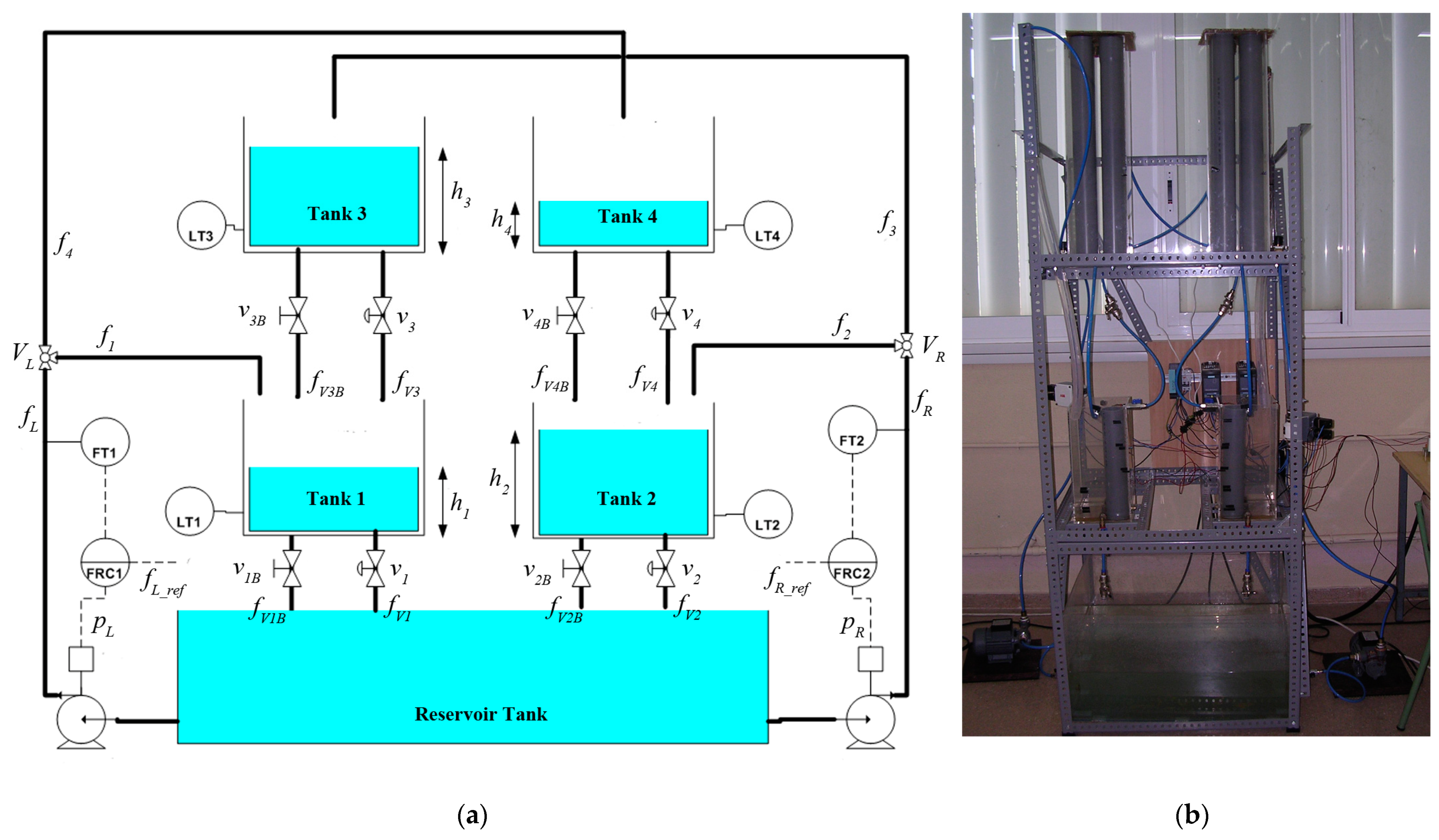
2. Laboratory Setup of the Quadruple-Tank System

The quadruple-tank system implemented in the Process Control laboratories of the University of Cordoba follows the scheme depicted in Figure 3a. The system consists of a reservoir tank at the bottom, and four tanks located on two levels: tanks 1 and 2 on the lower level, and tanks 3 and 4 on the upper level. The pump on the left (p_L) delivers a flow of water f_L from the reservoir tank, which is then split into two flows through the three-way valve (V_L): f₁ to tank 1 and f₄ to tank 4. The pump on the right (p_R) drives a flow rate f_R, which is then split by the V_R valve into f₂, which goes to tank 2, and f₃, which goes to tank 3. The tanks drain through manual valves that can be multiturn (v₁, v₂, v₃, and v₄) or on/off (v_1B, v_2B, v_3B, and v_4B). Tanks 1 and 2 divert water to the reservoir tank, whereas tanks 3 and 4 divert water to tanks 1 and 2, respectively. The tanks are coupled, meaning that, for example, when the pump on the right is used to fill tank 2, a portion of the total flow f_R goes to tank 3 and eventually reaches tank 1. The variables measured by the sensors are the water levels in the tanks (h₁, h₂, h₃, and h₄) and the total flow rates of each branch (f_L and f_R). The plant actuators are the frequency inverters that drive the pumps; therefore, the variables that can be manipulated are the frequency setpoints of these inverters, expressed as a percentage from 0 to 100%. However, as explained below, a secondary flow control loop is closed in each branch (left and right), so that the new manipulated signals are the flow references of each branch f_{L_ref} and f_{R_ref}.

Figure 3b shows a photograph of the real system. Its construction, unlike other similar plants, prioritized the use of industrial components over esthetics, resulting in larger dimensions. The elements that comprise it can be grouped into two categories: the hydraulic circuit and control system [33]. The hydraulic circuit is supported by a metallic structure and is composed of the following:

• Two 0.30 kW three-phase centrifugal pumps.
• Five methacrylate tanks. The reservoir tank measures 60 × 50 × 40 cm. The other four tanks have a square internal section of 19 × 19 cm² and a height of 35 cm for the lower tanks and 70 cm for the upper tanks. To improve the response time of the tanks, cylindrical tubes of constant section were introduced, as shown in Figure 3b. The cross-sectional area of the lower tanks, where only one tube is present, is 316.82 cm². The cross-sectional area of the upper tanks, where four tubes are present, is 184.29 cm².
• Two manual three-way diverter valves (V_L and V_R) are used to adjust the proportion of flow going to the lower tank in each branch. When in the 0% position, all the flow goes to the corresponding upper tank, so no water reaches the lower tank of that branch. Conversely, when in the 100% position, all the flow goes to the lower tank.
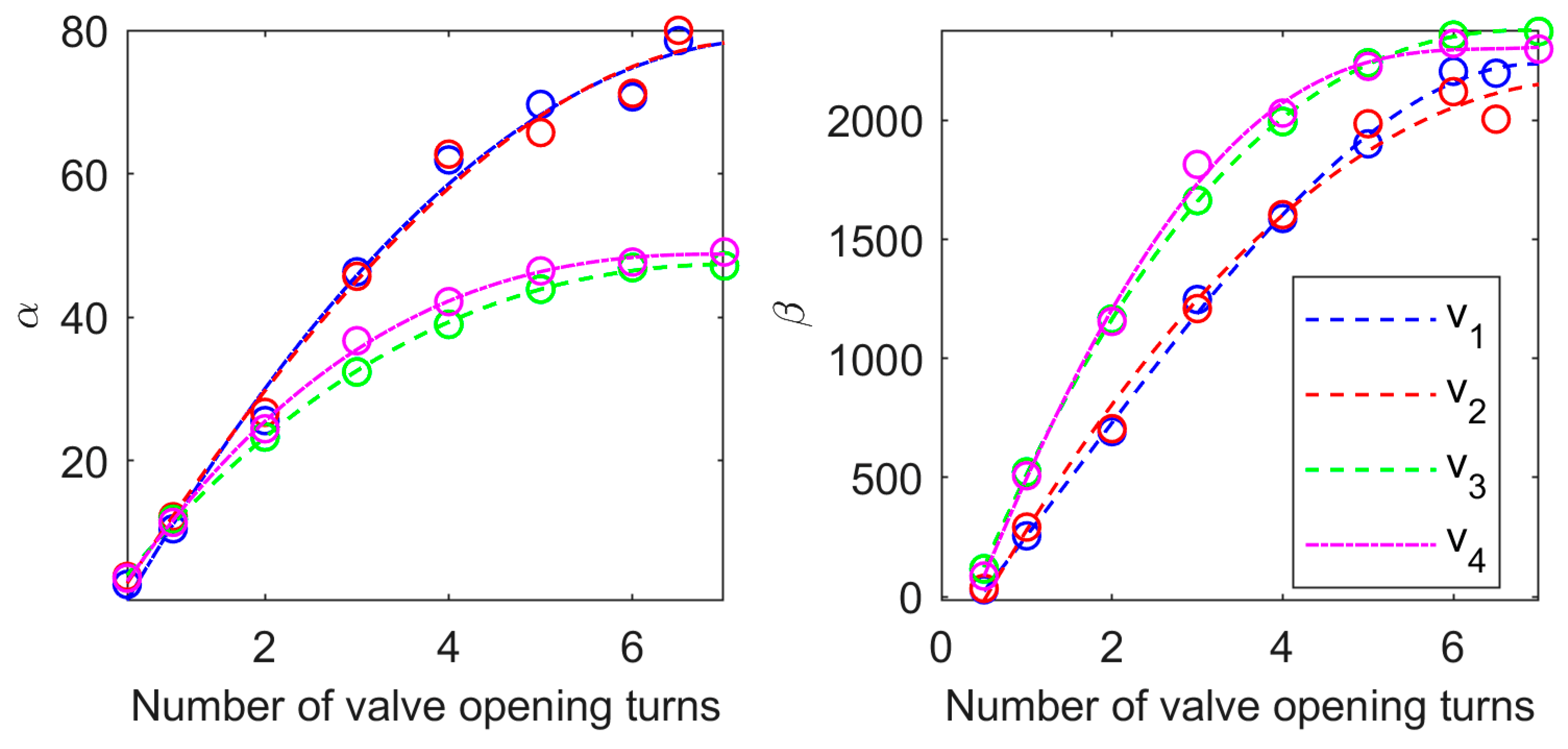
• Eight manual two-way valves are used to adjust the outflows of the four tanks. The multi-turn valves v₁, v₂, v₃, and v₄ can vary their opening degree with a total of up to six and a half or seven turns, depending on the valve. In contrast, valves v_1B, v_2B, v_3B, and v_4B have only two positions: fully closed or fully open.
• We use 10/8 mm polyurethane pipes and pipe fittings for connecting the different elements of the hydraulic circuit. In addition, two 40/32 mm PVC hoses are used to drain the inlet flows from the three-way valves to the lower tanks. Unlike the schematic shown in Figure 3a, the two outlets from each three-way valve are brought to the same height through 10/8 mm pipes. One branch goes to the corresponding upper tank, whereas the other branch goes to the 44/38 mm pipe so that from the upper height it drains without head loss. This design ensures that the two outlet branches of the three-way valves have similar head loss and that the flow distribution, depending on the position of the valve, is independent of the total inlet flow to the three-way valve.

The control system comprises measurement sensors, actuation devices, and control elements. These are as follows:

• Four upwelling diaphragm pressure transmitters for general applications. A measuring range of [0–0.1] bar, which is approximately a [0–100] cm water column. These transmitters were used to measure the water level in the four tanks.
• Two electromagnetic flow meters for measuring the total flow rates of the branches f_L and f_R. The measurement range is set to [0–200] cm³/s.
• Two frequency inverters to control the flow rate delivered by the pumps through a secondary control loop.
• An NI-DAQ 6035E data acquisition card to connect the process signals to a computer.
• A personal computer contains the acquisition card and the control software, which in this case is MATLAB 7.4 and its Real Time Windows Target toolbox. The configured sampling time is 1 s.

3. Modeling of the Quadruple-Tank System

This section explains the practical procedure proposed for obtaining a nonlinear model of the experimental plant from the modeling of its components using a grey-box approach. Two parts are considered:

• Pump dynamics and flow control: they determine the total flow rates of each branch (left and right) that the pumps drive from the reservoir tank to the other tanks.
• Dynamics of the four tanks: They determine the water level of each tank as a function of its corresponding inlet and outlet flow rates. The inlet flow rates depend on the total flow rate of each branch, the position of the three-way valves, and in the case of the lower tanks, the outlet flow rates of the upper tanks. The outflow of each tank depends on its water level and the degree of opening of its outlet valves.

Once the complete nonlinear model of the system is obtained and a configuration with the valves is set, it is linearized around an operating point to obtain a linear model. This linear model is represented as a matrix of transfer functions relating the water levels in tanks 1 and 2 to the total flows delivered by the pumps.

3.1. Dynamics of the Pumps and Secondary Flow Control Loops

The flow rates f_L and f_R sent to each branch (left and right) by the pumps are determined using this dynamic as a function of the percentage of operation of the frequency inverter of the corresponding pump, p_L or p_R. The transfer function in (3) models the relationship between the flow rate (cm³/s) of a branch, F(s), and the percentage of operation (%) of the corresponding pump drive, P(s), at approximately 50% operation.

$$F(s)=\frac{2.5e^{-0.74s}}{2.13s+1}P(s)$$

(3)

This transfer function may not be entirely accurate because of its nonlinear flow-pump characteristic, which varies depending on the operating point. However, its dynamics are fast enough compared to those of the tanks. Therefore, a secondary flow control loop was implemented in each branch using a proportional-integral (PI) controller to track flow references and reject disturbances. In addition, this approach prevents issues with pump performance fluctuation caused by changes in the reservoir tank level or pump heating. The implemented PI controller has a proportional gain K_P of 0.24%/(cm³/s) and an integral time constant T_I of 2.4 s. These values enable achieving responses with zero position error and a settling time of approximately 15 s, which is sufficiently fast to disregard these dynamics in comparison to those of the tanks. The controller was implemented in MATLAB/Simulink. The new process control signals are the flow references of each branch (f_{L_ref} and f_{R_ref}) in the range of [0–200] cm³/s. These signals are provided from a higher control level.

3.2. Tank Dynamics

Tank dynamics determine the inlet and outlet flow rates and the level of each tank. The dynamics are based on Bernoulli’s law and the laws of mass balance. The basic dynamics of tank k are given using the differential Equation (4). To determine the evolution of the water level h_k, it is only necessary to calculate the inflow f_{k_in} and outflow f_{k_out}, given the area A_k of the tank, which in this case is constant.

$${\dot{h}}_k=\left(f_{k\text{\_}in}-f_{k\text{\_}out}\right)/A_k$$

(4)

The inlet flow rates entering each tank are dependent on the total flow rate and the position of the three-way valve of the corresponding branch. The proportion of flow received by each of the two tanks associated with that branch was experimentally determined for different flow rates and positions of the three-way valve. For this purpose, several experiments were conducted, which consisted of filling the tanks with fixed values of both the reference flow rate and the position of the three-way valve. After the initial transient, the slope of the filling curve was determined to be linear. Multiplying the slope by the known area of the tanks gave the inlet flow rate for each tank. Because the total flow per branch is also known, the fraction going to the lower tanks can be determined.

Table 1. Proportion γ_L (%) of the flow rate f_L leading to tank 1 for different values of f_L and different positions of V_L.

VL (%)	fL (cm3/s)
	0	25	50	75	100	125	150	175	200
0	0	0	0	0	0	0	0	0	0
30	27	27.66	32.45	31.47	29.99	29.47	29.32	29.27	29.22
50	59	59.51	53.73	53.25	52.81	52.34	52.12	52.23	52.34
70	77	77.50	72.38	70.97	72.22	72.13	72.26	72.35	72.44
100	100	100	100	100	100	100	100	100	100

displays the ratio γ_L (in %) of the flow rate f_L directed to tank 1 for varying values of f_L and different positions of the left three-way valve V_L. Similarly,

Table 2. Proportion γ_R (%) of the flow rate f_R leading to tank 1 for different values of f_R and different positions of V_R.

VR (%)	fR (cm3/s)
	0	25	50	75	100	125	150	175	200
0	0	0	0	0	0	0	0	0	0
30	32	28.35	32.74	33.25	31.28	31.17	31	30.94	30.88
50	56	56	54.35	53.36	53.33	53.12	53.28	53.39	53.31
70	67	67.42	68.05	69.31	70.66	70.89	70.96	71.03	71.09
100	100	100	100	100	100	100	100	100	100

presents the ratio γ_R of the flow rate f_R directed to tank 2 for different values of f_R and various positions of the right three-way valve V_R. Figure 4 displays the percentages of these tables in graph form, exhibiting an almost linear trend.

From these tables, the surfaces in Figure 4 are fitted by planes whose equations are given in (5). These equations can be used to determine the fraction of flow that will enter the lower tank for any opening of the three-way valves (ranging from 0 to 100%) and any value of total flow of a branch (in the range 0 to 200 cm³/s); the remaining flow will enter the upper cross tank. Thus, using Equation (6) and the flow rates of each branch, we can calculate the inlet flow rate for each tank.

$$\begin{array}{l}{\gamma }_L=\left(1.813+1.013V_L-0.01066f_L\right)/100\\ {\gamma }_R=\left(1.123+0.9942V_R-0.001473f_R\right)/100\end{array}$$

(5)

$$\begin{array}{l}{f}_1={\gamma }_L{f}_L\hspace{1em}{f}_4=(1-{\gamma }_L)f_L\\ f_2={\gamma }_R{f}_R\hspace{1em}{f}_3=(1-{\gamma }_R)f_R\end{array}$$

(6)

The outflow rate of tank k is dependent on the degree of opening of its multiturn valve v_k, whether its valve v_kB is open or closed, and the water level in the tank. The outflow rate f_vk of each valve v_k was modeled according to Equation (7), where parameters α_k and β_k vary as a function of the manual opening of the valves, i.e., the number of opening turns. The water level in the tanks is measured from their base. However, because of the position of the tank outlet ports and the pressure sensor, not all of the measurement range is useful. If the level falls below the minimum value of 2 cm (h_min), the outflow becomes zero or negligible. Additionally, the equation becomes invalid if the tank overflows.

$$f_{Vk}\left(h_k\right)=\sqrt{{\alpha }_k{(\mathrm{v}}_k)h_k+{\beta }_k{(\mathrm{v}}_k)}\hspace{1em}{h}_{\min }<h_k<h_{k\text{\_}\max }$$

(7)

To obtain the coefficients α_k and β_k for each valve, a series of experiments were performed. The experiments consisted of emptying each tank from its maximum height h_{k_max} for different opening turns of the valve to be modeled. Once the level data in the tank were recorded, the emptying curve h(t) was fitted to a second-degree equation using least squares, as shown in (8). As shown in (9), this equation is derived with respect to time, and the time variable is then solved and substituted into (8). Next, the derivative of h is solved, resulting in an expression that relates the derivative of the tank level to the water level in the tank. Figure 5 shows the real emptying curves (in solid line) and their adjustments (in dashed line) for valves v₁, v₂, v₃, and v₄ when three turns have been opened.

$$h\left(t\right)=a{t}^2+bt+c$$

(8)

$$\begin{array}{c}\dot{h}=2at+b\hspace{1em}\to \hspace{1em}t=\frac{\dot{h}-b}{2a}\\ h=a{\left(\frac{\dot{h} - b}{2a}\right)}^2+b\left(\frac{\dot{h} - b}{2a}\right)+c\\ \dot{h}=\sqrt{4ah+(b^2-4ac)}\end{array}$$

(9)

As there is no inflow, the outflow of the valve is equal in the absolute value to the derivative of the water volume in the tank. Since the cross-sectional area (A) of each tank is constant, the derivative of the volume and the derivative of the water level are proportional. Therefore, given the derivative of the tank level, the outflow rate can be determined based on the water height. Thus, the outflow f_V can be determined using the expression in (10), which is similar to Equation (7). The parameters α and β are identified as a function of the parameters a, b, and c of the least squares optimization and the tank section A.

$$f_V=\left|\dot{V}\right|=A\left|\dot{h}\right|=\sqrt{A^{2}4ah+A^2(b^2-4ac)}=\sqrt{\alpha h+\beta }$$

(10)

Figure 6 displays the estimated values of α and β for the different multiturn valves in the form of circular dots. These values were obtained by conducting the same experiment for various valve openings. For each parameter α_k and β_k, a polynomial equation was fitted to determine the value as a function of the degree of valve opening. The fitting curves resulting from this analysis are also presented in Figure 6. The polynomial equations are provided in (11), and the fixed coefficients of the on/off valves v_1B, v_2B, v_3B, and v_4B when they are open are given in (12). There is significant symmetry between the valves on the left branch and their corresponding valves on the right side of the system. Most fitting polynomials in (11) are of order 3, but some have a different order to achieve a better fit. For certain parameters, the fitting polynomial of order 3 showed a downward trend at the end points, which does not correspond to reality. As the valve is opened further, both α and β should grow or at least not decrease.

$$\begin{array}{l}{\alpha }_1=-1.546v_1^2+23.56v_1-10.887\\ {\beta }_1=-5.44v_1^3+25.586v_1^2+435.568v_1-200.21\\ {\alpha }_2=-0.062v_2^3-0.666v_2^2+19.88v_2-6.847\\ {\beta }_2=-42.955v_2^2+655.43v_2-332.69\\ {\alpha }_3=0.044v_3^3-1.64v_3^2+16.66v_3-3.86\\ {\beta }_3=2.781v_3^3-96.075v_3^2+920.31v_3-312.86\\ {\alpha }_4=0.0942v_4^3-2.467v_4^2+20.55v_4-6.478\\ {\beta }_4=1.193v_4^4-13.276v_4^3-40.516v_4^2+905v_4-354.7\end{array}$$

(11)

$$\begin{array}{l}{\alpha }_{1B}=171.33,\hspace{1em}{\beta }_{1B}=2587.5,\hspace{1em}{\alpha }_{2B}=176.39,\hspace{1em}{\beta }_{2B}=2412.3\\ {\alpha }_{3B}=75.365,\hspace{1em}{\beta }_{3B}=3544.7,\hspace{1em}{\alpha }_{4B}=83.705,\hspace{1em}{\beta }_{4B}=3883.6\end{array}$$

(12)

3.3. Complete Nonlinear Model

The water level dynamics in each of the four tanks are calculated based on the differential equation of the tank given in (4), using the inlet and outlet flow rates. The upper tanks receive input only from the pumps, whereas the lower tanks receive input from both the pumps and outflow from their corresponding upper tanks. According to the plant schematic, the set of differential equations is as follows:

$$\begin{array}{l}{\dot{h}}_1=({\gamma }_L{f}_L+f_{V3}+f_{V3B}-f_{V1}-f_{V1B})/A_1\\ {\dot{h}}_2=({\gamma }_R{f}_R+f_{V4}+f_{V4B}-f_{V2}-f_{V2B})/A_2\\ {\dot{h}}_3=((1-{\gamma }_R)f_R-f_{V3}-f_{V3B})/A_3\\ {\dot{h}}_4=((1-{\gamma }_L)f_L-f_{V4}-f_{V4B})/A_4\end{array}$$

(13)

3.4. Linearization of the Nonlinear Model

This section derives the linear model in transfer functions by linearizing the nonlinear model around an operating point, based on the modular decomposition of the plant. The general equation in relative variables in the Laplace domain is obtained by linearizing (4) for each tank k around an operating point.

$$s{h}_k(\mathrm{s})=(f_{k\text{\_}in}(\mathrm{s})-f_{k\text{\_}out}(\mathrm{s}))/A_k$$

(14)

The equation above requires determination of the inlet and outlet flow rates for each tank. These flow rates are the sum of different components, as expressed in (13), depending on the tank. The outlet flow rates for each valve can be linearized using Taylor series expansion and truncated after the first-order term, as expressed in (15). The stationary values of the working point around which the model is obtained are f_{k_out,0} and h_k,0. After transitioning to the Laplace domain, we obtain Equation (16), where f_{k_out}(s) and h_k(s) are incremental variables with respect to the operating point. The transfer function is represented by a constant K_{k_out}.

$$f_{k\text{\_}out}-f_{k\text{\_}out,0}=\frac{{\alpha }_k}{2\sqrt{{\alpha }_k{h}_{k,0}+{\beta }_k}}(h_k-h_{k,0})$$

(15)

$$f_{k\text{\_}out}(\mathrm{s})=\frac{{\alpha }_k}{2\sqrt{{\alpha }_k{h}_{k,0}+{\beta }_k}}{h}_k(\mathrm{s})=K_{k\text{\_}out}{h}_k(\mathrm{s})$$

(16)

As previously stated, the pump flow rates are determined by secondary control loops that use their flow references as new inputs to the process. The response of these loops is very fast, and they have zero position error due to their integral action; therefore, their dynamics can be ignored. The ratio of flow from each branch to the corresponding lower tank, i.e., the fraction γ_L and γ_R, is of interest. These ratios depend on the position of the corresponding three-way valve and the total flow rate of its branch according to (5). For example, the partial derivative of γ_L with respect to the total flow rate f_{L_ref} of the left branch can be obtained using the expression in (5) for a fixed position of the three-way valve V_L. The linearization process is expressed in (17). The transfer function is given by K_{1_in}, which is another constant.

$$\begin{array}{l}{f}_1={\gamma }_L(f_{L\text{\_}ref})f_{L\text{\_}ref}\\ f_1-f_{1,0}={\left.\frac{\partial \left({\gamma }_L(f_{L\text{\_}ref})f_{L\text{\_}ref}\right)}{\partial f_{L\text{\_}ref}}\right|}_{f_{L\text{\_}ref,0}}\left(f_{L\text{\_}ref}-f_{L\text{\_}ref,0}\right)\\ f_1(s)=\left({\left.\frac{\partial {\gamma }_L(f_{L\text{\_}ref})}{\partial f_{L\text{\_}ref}}\right|}_{f_{L\text{\_}ref,0}}{f}_{L\text{\_}ref,0}+{\gamma }_L(f_{L\text{\_}ref,0})\right)f_{L\text{\_}ref}(s)=K_{1\text{\_}in}{f}_{L\text{\_}ref}(s)\end{array}$$

(17)

In the complementary part of that branch, specifically tank 4, the gain would be complementary to one, as shown in (18). Similar models can be obtained in the right-hand branch.

$$f_4(s)=(1-K_{1\text{\_}in})f_{L\text{\_}ref}(s)$$

(18)

To conclude, by linearizing the system in (13), using transfer functions similar to those in (14), (16)–(18), and solving for h₁(s) and h₂(s), we obtain the final expressions of the linear system, given using

$$\begin{array}{l}{h}_1(s)=\frac{\frac{K_{1\text{\_}in}}{(K_{1\text{\_}out}+K_{1B\text{\_}out})}}{\left(\frac{A_1}{\left(K_{1\text{\_}out}+K_{1B\text{\_}out}\right)}·s+1\right)}{f}_{L\text{\_}ref}(s)+\frac{\frac{(1-K_{2\text{\_}in})}{(K_{1\text{\_}out}+K_{1B\text{\_}out})}}{\left(\frac{A_3}{\left(K_{3\text{\_}out}+K_{3B\text{\_}out}\right)}s+1\right)\left(\frac{A_1}{\left(K_{1\text{\_}out}+K_{1B\text{\_}out}\right)}s+1\right)}{f}_{R\text{\_}ref}(s)\\ h_2(s)=\frac{\frac{(1-K_{1\text{\_}in})}{\left(K_{2\text{\_}out}+K_{2B\text{\_}out}\right)}}{\left(\frac{A_4}{\left(K_{4\text{\_}out}+K_{4B\text{\_}out}\right)}s+1\right)\left(\frac{A_2}{\left(K_{2\text{\_}out}+K_{2B\text{\_}out}\right)}s+1\right)}{f}_{L\text{\_}ref}(s)+\frac{\frac{K_{2\text{\_}in}}{(K_{1\text{\_}out}+K_{1B\text{\_}out})}}{\left(\frac{A_2}{\left(K_{2\text{\_}out}+K_{2B\text{\_}out}\right)}s+1\right)}{f}_{R\text{\_}ref}(s)\end{array}.$$

(19)

The transfer matrix of the linearized model can be expressed more concisely as follows:

$$G(s)=\left(\begin{array}{cc}\frac{\frac{T_1}{A_1}{K}_{1\text{\_}in}}{\left(T_{1}s+1\right)}& \frac{\frac{T_1}{A_1}(1-K_{2\text{\_}in})}{\left(T_{3}s+1\right)\left(T_{1}s+1\right)}\\ \frac{\frac{T_2}{A_2}(1-K_{1\text{\_}in})}{\left(T_{4}s+1\right)\left(T_{2}s+1\right)}& \frac{\frac{T_2}{A_2}{K}_{2\text{\_}in}}{\left(T_{2}s+1\right)}\end{array}\right),$$

(20)

where the outputs are h₁ and h₂ (in cm), and the inputs are f_{L_ref} and f_{R_ref} (in cm³/s). The time constants are given using

$$\begin{array}{l}{T}_1=\frac{A_1}{\left(K_{1\text{\_}out}+K_{1B\text{\_}out}\right)}\hspace{1em}{T}_3=\frac{A_3}{\left(K_{3\text{\_}out}+K_{3B\text{\_}out}\right)}\\ T_2=\frac{A_2}{\left(K_{2\text{\_}out}+K_{2B\text{\_}out}\right)}\hspace{1em}{T}_4=\frac{A_4}{\left(K_{4\text{\_}out}+K_{4B\text{\_}out}\right)}\end{array},$$

(21)

where the general expression of K_{k_out} is given in (16). The steady-state gain matrix and the relative gain matrix (RGA) of the system can be determined using Equations (22) and (23), respectively.

$$G(0)=\left(\begin{array}{cc}\frac{T_1}{A_1}{K}_{1\text{\_}in}& \frac{T_1}{A_1}(1-K_{2\text{\_}in})\\ \frac{T_2}{A_2}(1-K_{1\text{\_}in})& \frac{T_2}{A_2}{K}_{2\text{\_}in}\end{array}\right)=\left(\begin{array}{cc}{K}_{11}& K_{12}\\ K_{21}& K_{22}\end{array}\right)$$

(22)

$$RGA=\left(\begin{array}{cc}{K}_{1\text{\_}in}{K}_{2\text{\_}in}& \left(1-K_{1\text{\_}in}\right)\left(1-K_{2\text{\_}in}\right)\\ \left(1-K_{1\text{\_}in}\right)\left(1-K_{2\text{\_}in}\right)& K_{1\text{\_}in}{K}_{2\text{\_}in}\end{array}\right)\frac{1}{\left(K_{1\text{\_}in}+K_{2\text{\_}in}-1\right)}$$

(23)

The zeros of the multivariable process in (20) can be determined by finding the zeros of its determinant. According to [16], at least one of these zeros is always located in the left half-plane of the s-plane. If the condition in (24) is met, the other zero will be located in the right half-plane (RHP), which can lead to additional control challenges.

$$K_{1\text{\_}in}+K_{2\text{\_}in}<1$$

(24)

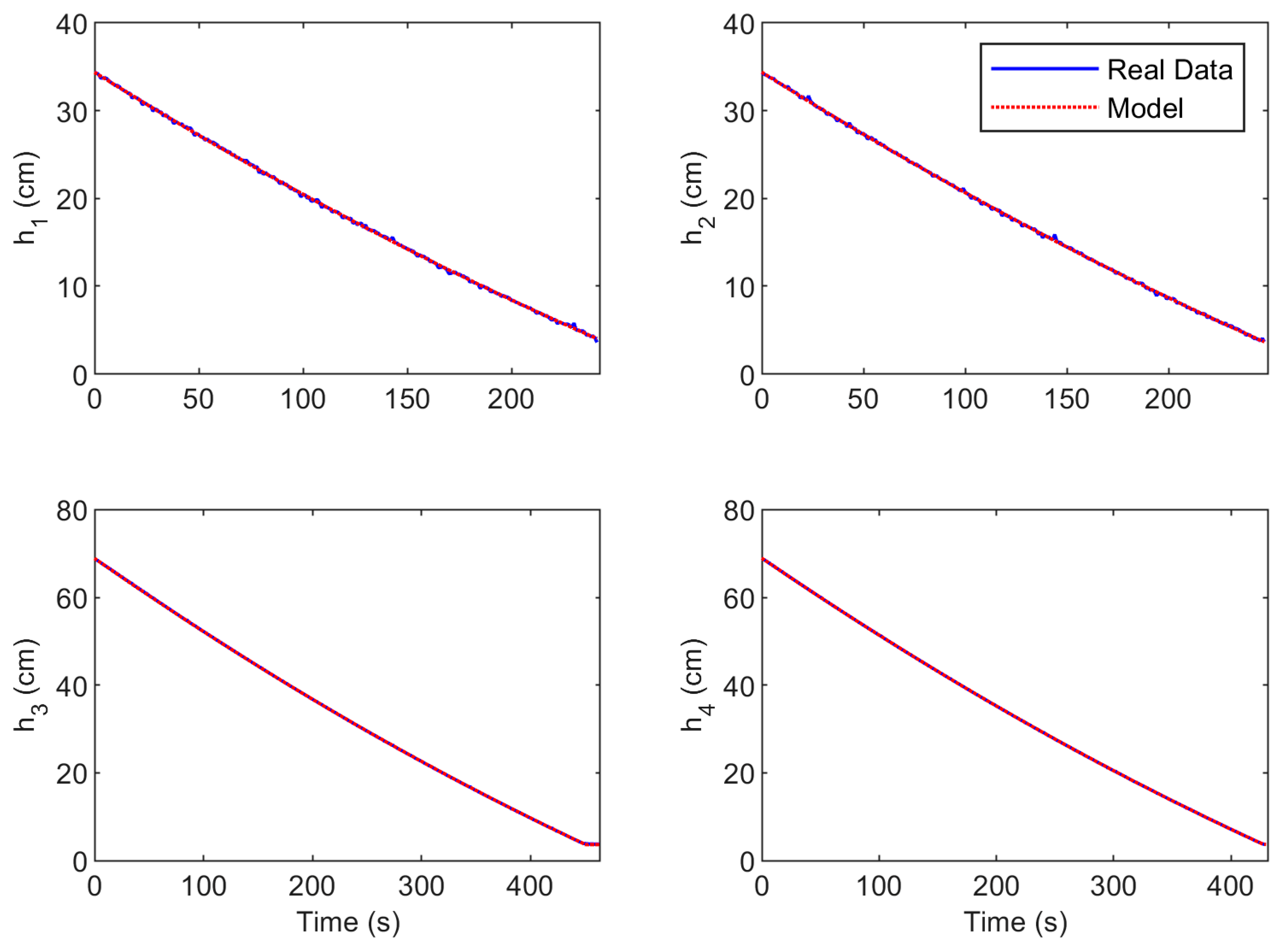
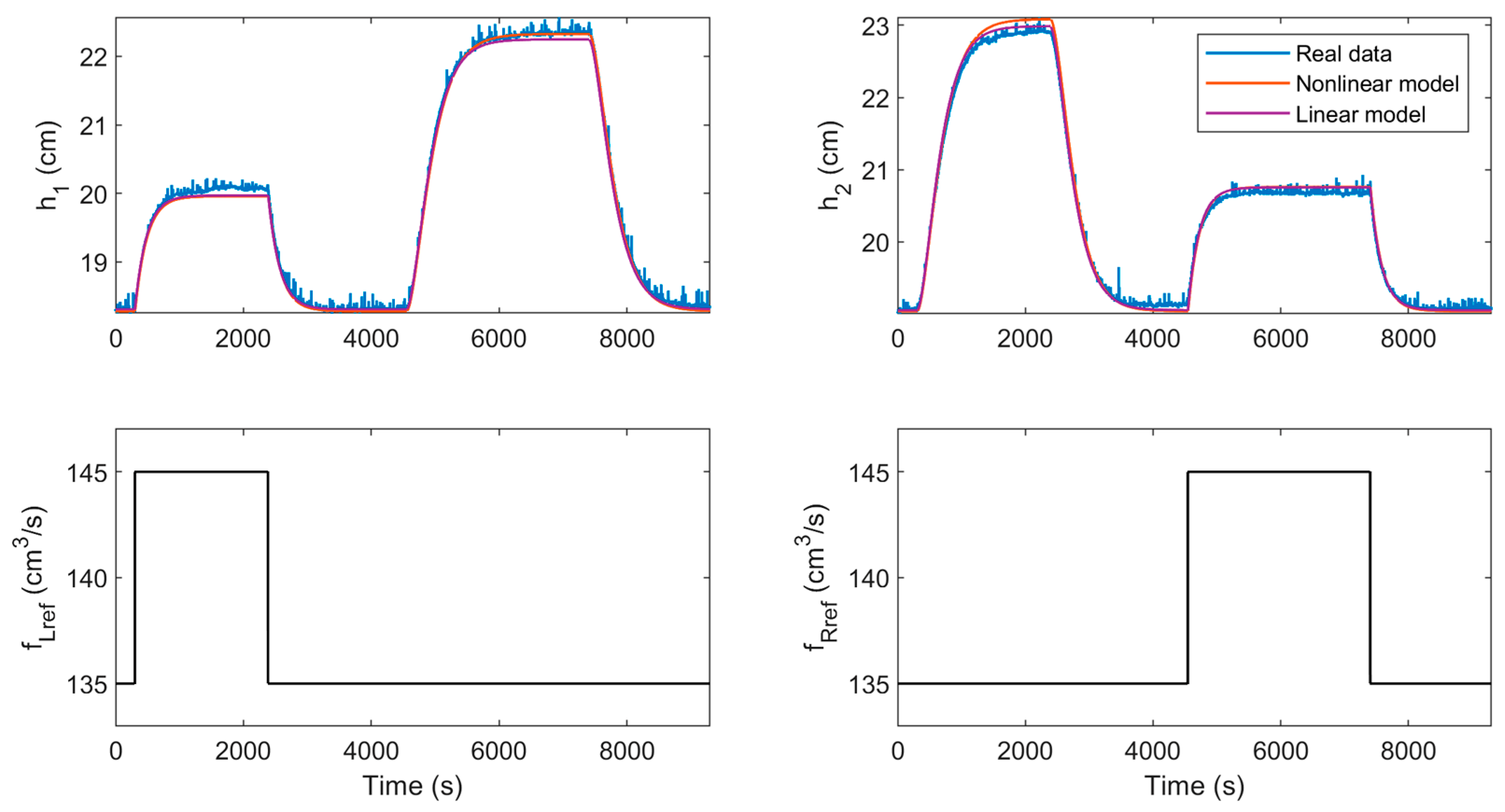
3.5. Validation of the Model

The experimental plant was configured to have a multivariable RHP zero by adjusting the different valves. Valves v₁ and v₂ are set to be six-turns open, while valves v₃ and v₄ are set to be one-turn open. All on–off valves are open. The three-way valves are set to be in the 30% position to provide more flow to the upper tanks. The reference flow rates selected as inputs were 135 cm³/s in both branches. The approximate stationary point is h₁ = 18 cm, and h₂ = 19 cm. The 2 × 2 matrix below represents the linear model obtained from the linearization of the nonlinear model, as described in (20):

$$G_{lin}(\mathrm{s})=\left(\begin{array}{cc}\frac{0.166}{179.7s+1}& \frac{0.394}{\left(179.7s+1\right)\left(238.1s+1\right)}\\ \frac{0.393}{\left(176.3s+1\right)\left(218s+1\right)}& \frac{0.17}{176.3s+1}\end{array}\right).$$

(25)

The non-principal diagonal elements of its RGA have a value of 1.22, and its stationary condition number is 2.5. Additionally, there is a non-minimum phase multivariable zero with a time constant of 169.78 s. The presence of the multivariable RHP zero imposes control limitations on the achievable bandwidth. To qualitatively validate the model accuracy, an open-loop experiment was conducted around the operating point using the experimental plant. To achieve this, pulses with an amplitude of 10 cm³/s are applied to the system inputs, starting from the operating point. Figure 7 compares the real data with the simulation performed using both linear and nonlinear models. Qualitatively, a good fit is observed. To quantitatively measure the fit, the root mean square error (RMSE) value of h₁ and h₂ is used, as defined in (26). These values are presented in

Table 3. RMSE values for the system level variables in the open-loop comparison.

Model	RMSE (h1) (cm)	RMSE (h2) (cm)
Nonlinear	0.062	0.093
Linear	0.071	0.066

. The results validate both the nonlinear and linear models.

$$\mathrm{RMSE}\left(h_i\right)=\sqrt{\frac{1}{N}{\displaystyle \sum _{k=1}^N{\left(h_{i\text{\_}\mathit{model}}\left(k\right)-h_{i\text{\_}real}\left(k\right)\right)}^2}}$$

(26)

The expressions obtained in (17) and (21) from linearizing the nonlinear model developed for a manual valve configuration can be used to directly obtain the parameters of the linear models around other operating points without the need to perform any experiments as would be the case with the black-box approach based on identification.

Table 4. Parameters of the linearized model for different operation points.

Operation Point				Model Parameters
fL_ref,0 (cm3/s)	fR_ref,0 (cm3/s)	h1,0 (cm)	h2,0 (cm)	K1_in	K2_in	T1 (s)	T2 (s)	T3 (s)	T4 (s)
135	135	18.3	19	0.293	0.306	179.7	176.3	238.1	218
150	150	27.1	28	0.290	0.305	199.9	196.7	264.7	242.8
125	125	12.9	13.6	0.295	0.306	166.2	162.7	220.5	201.5
125	165	29.1	20.2	0.295	0.304	204.1	179.1	291.3	201.6
170	130	22.2	33.2	0.286	0.306	188.8	207.5	229.3	276.0

lists the linear model parameters in (20) for different operating points.

4. Proposed Control Systems Using Decoupling

This section presents three multivariable control strategies for water levels in the lower tanks, starting from the linear model in (25). The strategies highlight the interaction and multivariable zero RHP problems. The proposed controllers are a multiloop PI control, a scheme that combines a multiloop PI control and a static decoupling network, and a centralized control that combines a multiloop PI control with simplified decoupling. Section 5 will present the results of each design, both in simulation and experimentally.

4.1. Multi-Loop PI Controller

The proposed control system in this section follows the decentralized control scheme depicted in Figure 1a. Since the non-diagonal elements of the process RGA are equal to 1.2, the water levels h₁ and h₂, which are controlled variables, are cross-paired with the flow rates f_R and f_L, respectively, which are the manipulated variables. The PI controllers in both loops are then tuned using a phase margin of 60° as the specification. PI controllers with the parallel structure given in (27) are used, where K_P is the proportional gain (cm²/s), K_I is the integral gain (cm²/s²), and h_{k_ref} are level references. When designing, it is important to consider that loop controllers may interact with each other. In this work, we used the iterative methodology proposed in [8], which adjusts the PI controllers in each iteration using single-input, single-output (SISO) methodologies for the equivalent open-loop process (EOP). This methodology considers the interaction with the other loop and the controller calculated in the previous step. The PI parameters for the h₂-f_L loop are K_P2 = 3.96 and K_I2 = 9.426 × 10⁻³. For the h₁-f_R loop, the PI parameters are K_P1 = 4.92 and K_I1 = 11.39 × 10⁻³.

$$\begin{array}{l}{f}_{R\text{\_}ref}\left(t\right)=K_{P1}\left(h_{1\text{\_}ref}\left(t\right)-h_1\left(t\right)\right)+K_{I1}{\displaystyle {\int }_0^t\left(h_{1\text{\_}ref}\left(t\right)-h_1\left(t\right)\right)dt}\\ f_{L\text{\_}ref}\left(t\right)=K_{P2}\left(h_{2\text{\_}ref}\left(t\right)-h_2\left(t\right)\right)+K_{I2}{\displaystyle {\int }_0^t\left(h_{2\text{\_}ref}\left(t\right)-h_2\left(t\right)\right)dt}\end{array}$$

(27)

4.2. Static Decoupling

This control approach follows the control scheme shown in Figure 1c and involves designing a static decoupling network from the process’ stationary state gain matrix G_lin(0) to reduce interaction at low frequencies [34]. The decoupling network is given using (28), which is the inverse of G_lin(0). Two PI controllers are then designed using the same methodology as above for the resulting apparent processes from the process and the static decoupler, i.e., the matrix Q(s) = G_lin(s)D₀. The multi-loop PI control employs diagonal pairing and a phase margin of 60° as specifications for both loops. The resulting PI parameters are K_P1 = 1.02 and K_I1 = 2.88 × 10⁻³ in the first loop, and K_P2 = 0.99 and K_I2 = 2.73 × 10⁻³ in the second loop.

$${\mathrm{D}}_0=\left(\begin{array}{cc}-1.343& 3.112\\ 3.104& -1.311\end{array}\right)$$

(28)

4.3. Simplified Decoupling

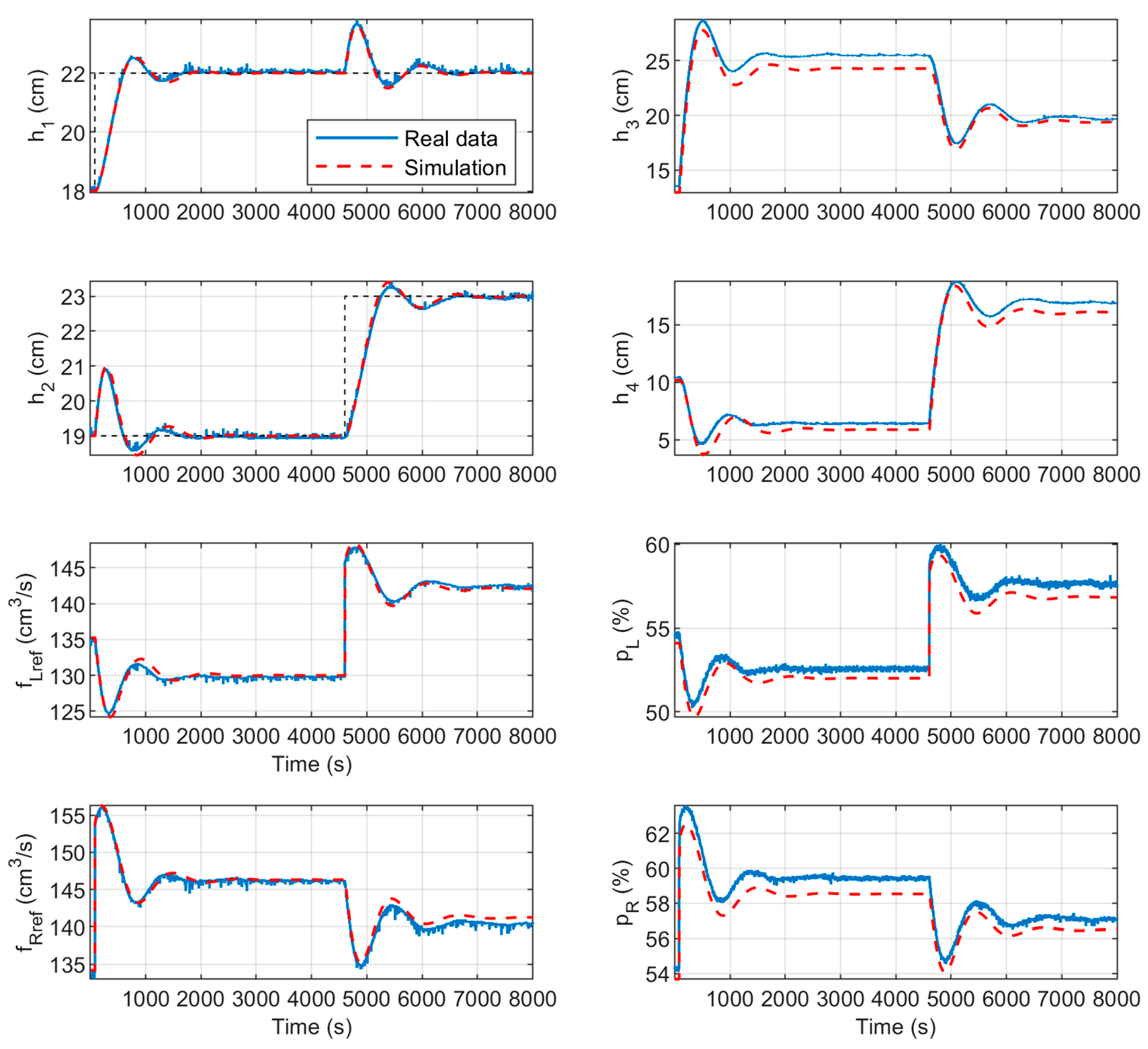
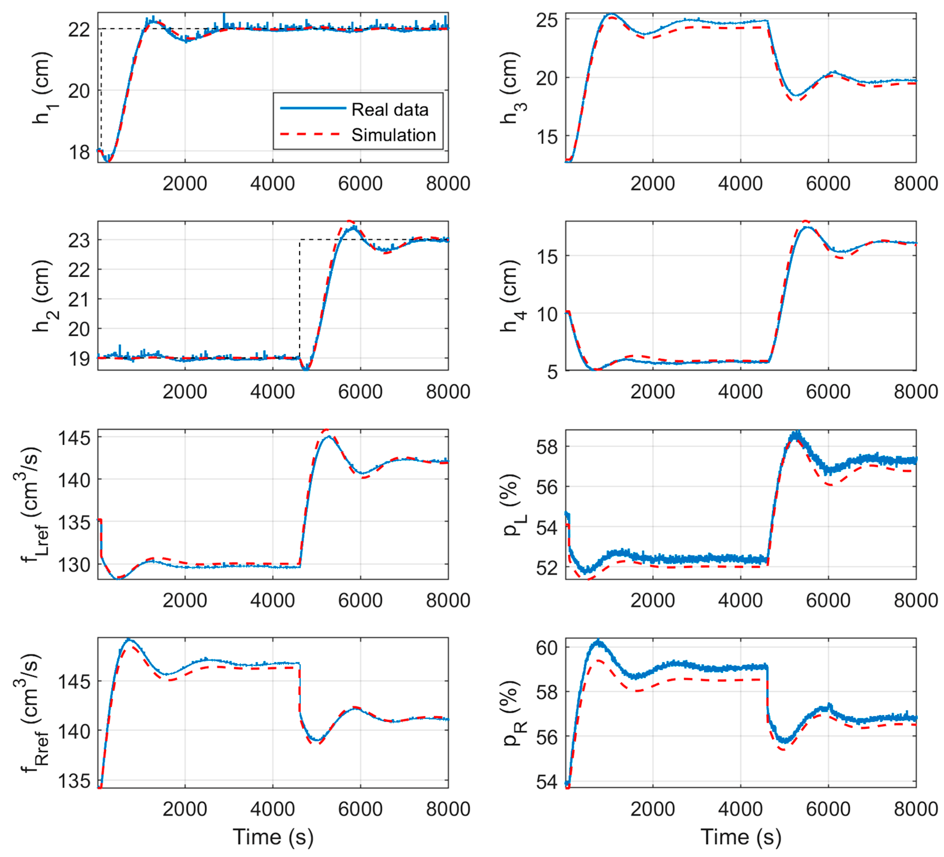
This decoupling control approach uses a dynamic decoupler to minimize interaction across all frequencies. The simplified decoupling method is employed, as described in (2), and is represented by the transfer matrix D_S(s) in (29). The resulting apparent process Q(s) is a diagonal matrix, as shown in (30), and does not exhibit any interaction. Two PI controllers are independently tuned for the corresponding elements of the resulting diagonal apparent process Q(s) = G_lin(s)·D_S(s), where the multivariable RHP zero of the process appears. The SISO methodology described in [35] is used with a phase margin of 60° as a specification in both loops. The resulting PI parameters are K_P1 = −1.09 and K_I1 = −1.873 × 10⁻³ in the first loop, and K_P2 = −1.23 and K_I2 = −2.15 × 10⁻³ in the second loop.

$$D_S(s)=\left(\begin{array}{cc}1& \frac{-2.373}{\left(238.1s+1\right)}\\ \frac{-2.312}{\left(218s+1\right)}& 1\end{array}\right)$$

(29)

$$Q(s)=\left(\begin{array}{cc}\frac{-0.7448\left(-169.78s+1\right)\left(68.13s+1\right)}{\left(179.7s+1\right)\left(238.1s+1\right)\left(218s+1\right)}& 0\\ 0& \frac{-0.7628\left(-169.78s+1\right)\left(68.13s+1\right)}{\left(176.3s+1\right)\left(218s+1\right)\left(238.1s+1\right)}\end{array}\right)$$

(30)

5. Results

This section applies the three designed control systems for both the nonlinear model and the real system. The simulated results are compared with the experimental results for each design and among the three designs. The test carried out in all three cases involves starting from levels of 18 and 19 cm in h₁ and h₂, respectively, and performing a step change of 4 cm at 80 s in the h₁ reference and at 4600 s in the h₂ reference. The test ends at 8000 s.

Figure 8, Figure 9 and Figure 10 display the simulation and experimental results for the designed control systems: decentralized, static decoupling, and simplified decoupling, respectively. Each figure presents the main variables of the control system on the left, including the levels of h₁ and h₂, and the total flow rates supplied by each pump, f_L and f_R, from top to bottom. On the right, secondary variables such as the tank levels h₃ and h₄, and the operation percentage of the pumps, p_L and p_R, are shown. Qualitatively, a good fit between the simulated and experimental data is observed in all three cases, particularly in the primary variables on the left. However, an offset between the simulated and experimental data is observed in the secondary variables on the right. The imprecise adjustment of the multiturn outlet valves may be the cause of the issues with the levels h₃ and h₄, whereas nonlinearities in the pumps may be responsible for the offset in the pump signals. To address this issue in the pumps, secondary loops were implemented in the QTS to regulate the flow rate of each pump based on the control signals of the proposed control systems. Thus, the absolute values of the percentage of pump usage are not crucial in the proposed model.

Table 5. RMSE values for the variables of the system in the different closed-loop systems.

Control System	RMSE
	h1 (cm)	h2 (cm)	fL (cm3/s)	fR (cm3/s)	h3 (cm)	h4 (cm)	pL (%)	pR (%)
Decentralized	0.06	0.09	0.5	0.65	0.92	0.7	0.68	0.81
Static decoupling	0.10	0.10	0.71	0.66	0.47	0.51	0.65	0.66
Simplified decoupling	0.06	0.11	0.44	0.46	0.41	0.30	0.45	0.53

displays the RMSE values of the system variables between the simulation and experimental results. These values quantitatively assess the degree of fit achieved with the proposed nonlinear model. The values are low enough to validate the proposed nonlinear model.

The experimental results were used to compare the three proposed control schemes.

Table 6. Performance indices for the different proposed control systems.

Control System	IAE (h1) (cms)			IAE (h2) (cms)			TV (fL) (cm3/s)	TV (fR) (cm3/s)
	Total	Tracking	Decoupling	Total	Tracking	Decoupling
Decentralized	2322	1444	878	2421	1566	855	535	715
Static decoupling	2682	1762	920	2380	1795	585	500	514
Simplified decoupling	3003	2882	121	3023	2818	205	163	168

displays the integrated absolute error (IAE) of tank levels 1 and 2 in relation to their references. The total value is calculated using all experimental data, while the tracking value is calculated using only the values corresponding to reference changes in that water level, providing information on the IAE of reference tracking. The decoupling value is calculated using data corresponding to changes in the reference of the other loop, providing information on the decoupling performance. Table 6 displays the total rate of variation (TV) values of the control signals, which are related to the control effort. The expressions for IAE and TV are presented in (31).

$$\mathrm{ITAE}\left(h_k\right)={\displaystyle {\int }_0^t\left|h_{k\text{\_}ref}\left(t\right)-h_k\left(t\right)\right|}dt\hspace{1em}\mathrm{TV}\left(f_K\right)={\displaystyle {\int }_0^t\left|\frac{d\left(f_K\left(t\right)\right)}{dt}\right|}dt$$

(31)

Decentralized control achieves a fast response to changes in the reference with a settling time of approximately 2000 s. However, it exhibits a significant interaction in the opposite loop when such changes occur. Therefore, testing the use of decoupled control schemes was justified. Static decoupling control shows a similar reference tracking response, albeit slightly slower, as reflected by the higher IAE values for tracking. However, the decentralized control fails to achieve the same level of decoupling as loop 2, which has an IAE value that is 35% lower. Furthermore, loop 2 has lower TV values, particularly in f_R, which is 28% lower. Static decoupling cannot eliminate all interactions because it is not a dynamic decoupler. The simplified decoupling control achieves nearly perfect decoupling by eliminating interaction in both loops. Its small IAE values for decoupling are 86% lower than those of the other control schemes in loop 1, and 76% and 65% lower in loop 2 compared to decentralized control and static decoupling, respectively. The decoupling process results in a slower response time, with a settling time of approximately 3000 s. This is evidenced by the higher IAE values for tracking, which are approximately twice as high as those of decentralized control and 60% higher than those of control with static decoupling. The inferior response to reference tracking is a result of the constraint imposed by the multivariable RHP zero, which appears in the apparent process elements Q(s) when simplified decoupling is applied. This RHP zero is responsible for the inverse response to changes in the reference. In this QTS configuration, there is a trade-off between the peak of the inverse response and the interaction in the other loop due to the RHP zero. Regarding TV values, the simplified decoupling method has the lowest values, which are approximately 70% lower than those of the decentralized control.

6. Conclusions

This paper presents a practical grey-box modeling procedure for the quadruple-tank system used at the University of Cordoba. The proposed method overcomes the unrealistic assumptions made in other models, such as assuming linear behavior of the actuators and three-way valves. This results in a more realistic, configurable, and reproducible model. The proposed grey-box approach highlights the following points, which can also be useful for modeling other systems with liquid tanks:

• Secondary control loops are suggested to regulate the flow rate delivered by each pump, making the new control variables the references for those flow rates. The controllers have integral action, resulting in zero stationary error. In addition, the response of these loops is much faster than the dynamics of the tanks, allowing for the requested changes to the flow rate to be almost instantaneous. This approach helps to avoid pump nonlinearities.
• The proposed method for modeling the outflows of the tanks is based on level data measured during the experience of emptying the tank and is expressed using the Bernoulli equation.
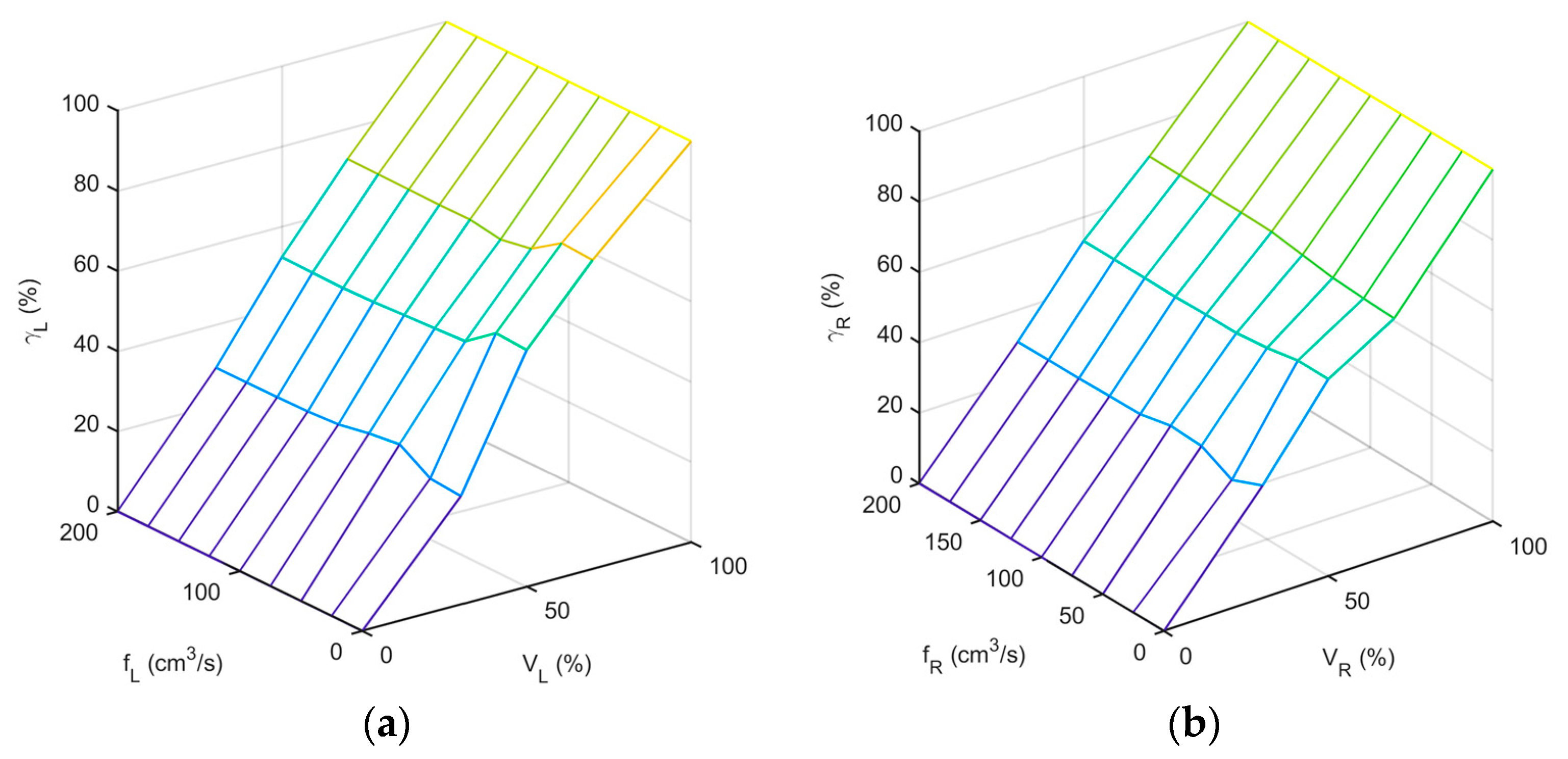
• The percentage of flow diverted to the lower tanks from the three-way valves is modeled using planes as a function of inlet flow and valve position, based on tank filling experiences. To facilitate modeling of these valves, it is useful for the outlet pipes of the three-way valve to have the same length in the construction of the real plant in order to equalize the head losses of both outlet sections. Thus, the distribution of flow is less affected by the total inlet flow, depending on the valve position.

The proposed grey-box approach has resulted in the development of a nonlinear model and has been developed so that it can be adjusted based on valve positions to exhibit little or large interactions, or RHP zero. This model has allowed for the derivation of general expressions of the linearized process model around a generic operating point. These expressions provide an accurate linear model for designing controls at different operating points without the need for new experiments. In contrast, the black-box approach requires experiments at each operating point to obtain a linear model. In addition, the generic expressions of the linear model of the process allow easy implementation of more advanced control strategies such as adaptive control using gain scheduling. For this study, a configuration with a large interaction and RHP zero was selected. Different control strategies were designed based on the linearized model at one operating point and applied to both the nonlinear model and the real process. The validity of the nonlinear model is demonstrated by comparing the simulations and experimental results. The results and conclusions obtained from applying different control designs in the simulation are extrapolated to the real system.

Therefore, it can be concluded that both the real system and the nonlinear model are valuable tools for research and teaching. They offer the opportunity to simulate and experiment with highly interacting processes, including their control systems. The system interactions provide opportunities to test new control theories for robustness and performance with reasonable time and effort. This study presents three control schemes: a decentralized PI control, a static decoupled control, and a simplified decoupled control. We investigated the bandwidth limitation of the control system caused by a multivariable RHP zero when applying perfect decoupling, such as the simplified decoupled control, in both loops. The reference tracking response of the decentralized control is faster, but it comes at the cost of showing large interaction in the opposite loop. It is worth noting that this plant has been successfully used for practical work by students of control courses, as well as by our research group.

References

1. Aranda-Cetraro, I.; Pérez-Zúñiga, G.; Rivas-Pérez, R.; Sotomayor-Moriano, J. Nonlinear Robust Control by a Modulating-Function-Based Backstepping Super-Twisting Controller for a Quadruple Tank System. Sensors 2023, 23, 5222. [Google Scholar] [CrossRef]
2. Hu, Z.; Wang, J.; Li, D.; Qin, J. Application of Desired Dynamic Equation Method in Simulation of Four-Tank System. In Proceedings of the 2012 International Conference on Systems and Informatics, ICSAI 2012, Yantai, China, 19–20 May 2012; pp. 366–370. [Google Scholar]
3. Harsha, S.; Vinod, D.; Saikrishna, P.S. Identification and Multi-Objective H∞ Control Design for a Quadruple Tank System. In Proceedings of the 2019 IEEE 7th Conference on Systems, Process and Control, ICSPC 2019, Melaka, Malaysia, 13–14 December 2019; pp. 70–75. [Google Scholar] [CrossRef]
4. Sohlberg, B.; Jacobsen, E.W. Grey Box Modelling—Branches and Experiences; IFAC: New York, NY, USA, 2008; Volume 41, ISBN 9783902661005. [Google Scholar]
5. Bohlin, T. Practical Grey-Box Process Identification; Springer: Berlin/Heidelberg, Germany, 2006; ISBN 9781846284021. [Google Scholar]
6. Skogestad, S.; Postlethwaite, I. Multivariable Feedback Control: Analysis and Design; Wiley: Hoboken, NJ, USA, 2007; ISBN 978-0-470-01168-3. [Google Scholar]
7. Luyben, W.L. Simple Method for Tuning SISO Controllers in Multivariable Systems. Ind. Eng. Chem. Process Des. Dev. 1986, 25, 654–660. [Google Scholar] [CrossRef]
8. Garrido, J.; Ruz, M.L.; Morilla, F.; Vázquez, F. Iterative Method for Tuning Multiloop Pid Controllers Based on Single Loop Robustness Specifications in the Frequency Domain. Processes 2021, 9, 140. [Google Scholar] [CrossRef]
9. Bristol, E. On a New Measure of Interaction for Multivariable Process Control. IEEE Trans. Autom. Control 1966, 11, 133–134. [Google Scholar] [CrossRef]
10. Shinskey, F.G. Process Control Systems: Application, Design, and Tuning, 4th ed.; McGraw-Hill Inc.: New York, NY, USA, 1996; ISBN 0-07-057101-5. [Google Scholar]
11. Skogestad, S. Advanced Control Using Decomposition and Simple Elements. Annu. Rev. Control 2023, 56, 100903. [Google Scholar] [CrossRef]
12. Wang, Q.-G. Decoupling Control; Springer: Berlin/Heidelberg, Germany, 2003; ISBN 978-3-540-44128-1. [Google Scholar]
13. Liu, L.; Tian, S.; Xue, D.; Zhang, T.; Chen, Y.Q.; Zhang, S. A Review of Industrial MIMO Decoupling Control. Int. J. Control Autom. Syst. 2019, 17, 1246–1254. [Google Scholar] [CrossRef]
14. Waller, M.; Waller, J.B.; Waller, K.V. Decoupling Revisited. Ind. Eng. Chem. Res. 2003, 42, 4575–4577. [Google Scholar] [CrossRef]
15. Zhu, Q.; Li, R.; Zhang, J. Model-Free Robust Decoupling Control of Nonlinear Nonaffine Dynamic Systems. Int. J. Syst. Sci. 2023, 54, 2590–2607. [Google Scholar] [CrossRef]
16. Zhu, Q.; Li, R.; Zhang, J.; Shi, B. Model-Free Robust Decentralised Control of Multi-Input-Multi-Output Nonlinear Interconnected Dynamic Systems. JVC/J. Vib. Control 2023. [Google Scholar] [CrossRef]
17. Johansson, K.H.; Nunes, J.L.R. A Multivariable Laboratory Process with an Adjustable Zero. In Proceedings of the American Control Conference, Philadelphia, PA, USA, 26 June 1998; Volume 4, pp. 2045–2049. [Google Scholar] [CrossRef]
18. Johanssont, K.H.; Horcht, A.; Wijkt, O.; Hanssont, A. Teaching Multivariable Control Using the Quadruple-Tank Process. In Proceedings of the 38th IEEE Conference on Decision and Control, Phoenix, AZ, USA, 7–10 December 1999. [Google Scholar]
19. Johansson, K.H. The Quadruple-Tank Process: A Multivariable Laboratory Process with an Adjustable Zero. IEEE Trans. Control Syst. Technol. 2000, 8, 456–465. [Google Scholar] [CrossRef]
20. Meng, X.; Yu, H.; Xu, T.; Wu, H. Disturbance Observer and L2-Gain-Based State Error Feedback Linearization Control for the Quadruple-Tank Liquid-Level System. Energies 2020, 13, 5500. [Google Scholar] [CrossRef]
21. Shneiderman, D.; Palmor, Z.J. Properties and Control of the Quadruple-Tank Process with Multivariable Dead-Times. J. Process Control 2010, 20, 18–28. [Google Scholar] [CrossRef]
22. Gatzke, E.P.; Meadows, E.S.; Wang, C.; Doyle, F.J. Model Based Control of a Four-Tank System. Comput. Chem. Eng. 2000, 24, 1503–1509. [Google Scholar] [CrossRef]
23. Kozáková, A.; Čápková, R.; Kozák, Š. Decentralized QFT Controller Design Based on the Equivalent Subsystems Method. Electronics 2023, 12, 3658. [Google Scholar] [CrossRef]
24. Das Neves, G.P.; Barbosa, F.S.; Costa, P.S.; Angelico, B.A. Discrete Time LQG/LTR Applied to a Practical Quadruple Tank System. In Proceedings of the 2016 IEEE Conference on Control Applications, CCA 2016, Buenos Aires, Argentina, 19–22 September 2016; pp. 1232–1237. [Google Scholar] [CrossRef]
25. Piñón, A.; Favela-Contreras, A.; Beltran-Carbajal, F.; Lozoya, C.; Dieck-Assad, G. Novel Strategy of Adaptive Predictive Control Based on a MIMO-ARX Model. Actuators 2022, 11, 21. [Google Scholar] [CrossRef]
26. Oyehan, I.A.; Osunleke, A.S.; Ajani, O.O. Closed-Loop Stability of a Non-Minimum Phase Quadruple Tank System Using a Nonlinear Model Predictive Controller with EKF. ChemEngineering 2023, 7, 74. [Google Scholar] [CrossRef]
27. Alvarado, I.; Limon, D.; Muñoz De La Peña, D.; Maestre, J.M.; Ridao, M.A.; Scheu, H.; Marquardt, W.; Negenborn, R.R.; De Schutter, B.; Valencia, F.; et al. A Comparative Analysis of Distributed MPC Techniques Applied to the HD-MPC Four-Tank Benchmark. J. Process Control 2011, 21, 800–815. [Google Scholar] [CrossRef]
28. Gurjar, B.; Chaudhari, V.; Kurode, S. Parameter Estimation Based Robust Liquid Level Control of Quadruple Tank System—Second Order Sliding Mode Approach. J. Process Control 2021, 104, 1–10. [Google Scholar] [CrossRef]
29. Biswas, P.P.; Srivastava, R.; Ray, S.; Samanta, A.N. Sliding Mode Control of Quadruple Tank Process. Mechatronics 2009, 19, 548–561. [Google Scholar] [CrossRef]
30. Eltantawie, M.A. Decentralized Neuro-Fuzzy Controllers of Nonlinear Quadruple Tank System. SN Appl. Sci. 2019, 1, 39. [Google Scholar] [CrossRef]
31. Thamallah, A.; Sakly, A.; M’Sahli, F. A New Constrained PSO for Fuzzy Predictive Control of Quadruple-Tank Process. Measurement 2019, 136, 93–104. [Google Scholar] [CrossRef]
32. Son, N.N. Level Control of Quadruple Tank System Based on Adaptive Inverse Evolutionary Neural Controller. Int. J. Control Autom. Syst. 2020, 18, 2386–2397. [Google Scholar] [CrossRef]
33. Castelo, G.; Garrido, J.; Vazquez, F. Ajuste, Configuración y Control de Cuatro Tanques Acoplados. In Proceedings of the Jornadas de Automática 2008, Tarragona, Spain, 3–5 September 2008. [Google Scholar]
34. Lee, J.; Kim, D.H.; Edgar, T.F. Static Decouplers for Control of Multivariable Processes. AIChE J. 2005, 51, 2712–2720. [Google Scholar] [CrossRef]
35. Garrido, J.; Ruz, M.L.; Morilla, F.; Vázquez, F. Interactive Tool for Frequency Domain Tuning of PID Controllers. Processes 2018, 6, 197. [Google Scholar] [CrossRef]
Figure 1. Multivariable control approaches: (a) decentralized, (b) centralized, and (c) centralized, combining decoupling network and diagonal control.
Actuators 13 00087 g001
Figure 2. 2 × 2 control system combining a decoupler and a diagonal controller.
Actuators 13 00087 g002
Figure 3. (a) Schematic of the quadruple-tank system in the laboratory; (b) real quadruple-tank process in the laboratory.
Actuators 13 00087 g003
Figure 4. Experimental measurements of the flow fraction to the lower tanks as a function of the total flow rate of each branch and the position of the three-way valve: (a) right branch and (b) left branch.
Actuators 13 00087 g004
Figure 5. Real emptying curves and their adjustment for valves v1, v2, v3, and v4 when the degree of opening is 3 turns.
Actuators 13 00087 g005
Figure 6. Values of α and β of the valves v1, v2, v3, and v4 for different opening turns and their polynomial fitting.
Actuators 13 00087 g006
Figure 7. Open-loop comparison of the linear and nonlinear models with the real process.
Actuators 13 00087 g007
Figure 8. Experimental and simulated decentralized control results.
Actuators 13 00087 g008
Figure 9. Experimental and simulated static decoupling control results.
Actuators 13 00087 g009
Figure 10. Experimental and simulated simplified decoupling control results.
Actuators 13 00087 g010