Article

Dynamic Output Feedback of Second-Order Systems: An Observer-Based Controller with Linear Matrix Inequality Design

by
Danielle Gontijo
1,
José Mário Araújo
2,*,
Luciano Frezzato
1,3 and
Fernando de Oliveira Souza
1,3
1
Programa de Pós-Graduação em Engenharia Elétrica, Universidade Federal de Minas Gerais, Belo Horizonte 31270-901, MG, Brazil
2
Grupo de Pesquisa em Sinais e Sistemas, Instituto Federal da Bahia, Salvador 40301-015, BA, Brazil
3
Departamento de Engenharia Eletrônica, Universidade Federal de Minas Gerais, Belo Horizonte 31270-901, MG, Brazil
*
Author to whom correspondence should be addressed.
Actuators 2024, 13(6), 216; https://doi.org/10.3390/act13060216
Submission received: 7 May 2024 / Revised: 4 June 2024 / Accepted: 7 June 2024 / Published: 9 June 2024
(This article belongs to the Special Issue Dynamics and Control of Underactuated Systems)

Abstract

:
This paper presents an observer-based dynamic output-feedback controller design procedure using linear matrix inequality (LMI) optimization for second-order systems with uncertainty and persistent perturbation in the states. Using linear-quadratic criteria, cost functions are minimized in a two-stage procedure to compute optimal state-feedback gains, and observer gains are coupled into a dynamic output-feedback optimal controller. The LMI set used in the two stages is matrix inversion free, a key issue for polytope formulation when uncertainty is present. The approach is tested in a mobile inverted pendulum robotic platform, and the effectiveness is verified in this underactuated and undesensed case.

1. Introduction

Second-order differential equations arise in several system modeling, such as electrical, electromechanical, and mechanical systems. Also, they are commonly used in structural, vibration, multi-body systems, and robotic modeling and control [1,2,3,4].
In several practical applications, the allocation of sensors to cover all the degrees of freedom may be expensive, or the physical location of certain degrees of freedom may be hard to access. In such scenarios, if the system model is observable from the measured outputs, the reconstruction of the state is possible by using functional observers. Since asymptotic observers for linear systems exhibit, in general, a separation principle, the estimated states from the observer can be applied to feedback control purposes. Such controllers are known as dynamic output-feedback controllers. Observers in states-pace and descriptor models have been covered over five decades [5,6,7,8,9,10,11,12]; more recently, second-order observers were described and applied to control structural, vibration, or multi-body systems [13,14].
Control tasks with underactuated systems constitute a challenge since the number of actuators is less than the number of degrees of freedom in the system, that is, the well-known configuration variables [15,16]. Although it demands a more complex design of the controller, the adoption of an underactuated configuration improves the lightweight of the global structure and reduces the total cost of the project. Another situation in which underactuated systems rise is the fault-tolerant control design [15,17]. If the underactuated structure is also undersensed or the measurements are severely noisy, reconstruction of the state vector using state observers can be of great significance to recover the controller’s effectiveness. Some works in control literature approach this problem in its essence [18,19].
This work presents a solution for the design of dynamic output-feedback controllers for second-order systems using a functional descriptor observer and an optimization problem to achieve closed-loop stability and performance criteria, among that, robustness against uncertainty parameters, persistent exogenous perturbations, and LQR quadratic indices for the state vector and control effort. The design methodology is a two-stage convex optimization procedure that computes the robust state-feedback gains at the first stage and then the robust gains of the observer in the second stage, anchored in a separation principle for error and feedback-controlled state dynamics. The proposed linear matrix inequality (LMI) formulation does not use matrix inversion, a point that can be involved when uncertainty is present. Other advanced control methods can also tackle uncertainties, but some limitations are inherent when the uncertainty is modeled. For instance, in model predictive control (MPC), the uncertainty must be incorporated into the solution of the optimization problem that computes the control sequence using LMI, tubes, or min-max techniques [20], with a reasonable increment of computational cost in that cases in comparison with uncertainty-free MPC; some contributions to robust sliding-mode control (SMC) for singular or descriptor systems can be encountered in the literature but with uncertainties considered only in part of the system matrices [21,22]. As far as the authors’ knowledge, there are no available methods in the literature to design dynamic output-feedback controllers for descriptor systems subject to polytopic uncertainties in all matrices.
Notation throughout this paper is standard. Let the scalar j = 1 and R m × n be the set of m × n real matrices. If w ( t ) is a random value, E { w } denotes its expected value or expectation. For a matrix X, denote its transpose by X T and its inverse by X 1 . If X is square and symmetric, then X > 0 ( X 0 ) indicates that X is positive (semi) definite; similarly, X < 0 ( X 0) indicates that X is negative (semi) definite. The notation cov denotes convex hull, and diag { x 1 , , x n } is used for a diagonal matrix whose diagonal entries, starting in the upper left corner, are x 1 , , x n . Moreover, for any square matrix X, we define the operator sm { X } = X + X T . Let I n ( 0 n ) be the identity (zero) matrix with dimension n × n and 0 n × m the zero matrix with dimension n × m ; throughout this paper, such subscripts will be suppressed whenever the dimension is evident from the context.

2. Preliminaries and Problem Formulation

Consider the class of second-order systems described by the linear model:
M z ¨ ( t ) + D z ˙ ( t ) + S z ( t ) = B u ( t ) + F w ( t )
where the non-singular matrices M, D, S R n × n , B R n × m , F R n × p are the model matrices, z ( t ) R n is the state vector, u ( t ) R m is the control input, and w ( t ) R p is the exogenous disturbance vector, which is assumed to be a white noise with zero mean, uncorrelated in time and with a covariance matrix W > 0 , that is
E { w ( t ) } = 0 and E { w ( t ) w T ( τ ) } = W δ ( t τ ) , for τ > 0 .
Defining the state variables
x 1 ( t ) = z ( t ) and x 2 ( t ) = z ˙ ( t )
and rewriting Model (1) as an augmented first-order one yields the following augmented descriptor model
E x ˙ ( t ) = A x ( t ) + B u u ( t ) + B w w ( t )
with x T ( t ) = [ x 1 T ( t ) x 2 T ( t ) ] , and
E = I n 0 n 0 n M , A = 0 n I n S D , B u = 0 n × m B , B w = 0 n × p F .
A short-hand notation for the descriptor system (3) is given as
S E A B u B w .
In case S is uncertain, we add the argument α in it, and we assume that S ( α ) belongs to the polytopic set Δ cov { S 1 , S 2 , , S N } . In other words, Δ is defined as the set of all matrices obtained by the convex combination of their vertices
Δ = S ( α ) : S ( α ) = i = 1 N α i S i , α Ξ
where
Ξ α : α i 0 , i = 1 N α i = 1 .
The vertices of system S ( α ) are determined by combining the extreme values of its uncertain parameters.
Generally, in actual applications, the internal state of a system is only partially available for feedback. Hence, in this work, we propose an observer-based controller whose control signal is obtained through estimates of the system’s internal state. The observer structure and control signal u ( t ) are such that
E ^ x ^ ˙ ( t ) = A ^ x ^ ( t ) + B ^ u u ( t ) + E ^ L ( y ^ ( t ) y ( t ) ) y ^ ( t ) = C x ^ ( t ) u ( t ) = K x ^ ( t )
where the matrices with the hat symbol (∧) are given (which can be chosen as the mean matrix of the respective system uncertain matrix). The gains K and L are parameters to be determined.
Combining (3) and (7), we have
E ^ 0 0 E i x ^ ˙ x ˙ = A ^ + B ^ u K 0 B u , i K A i x ^ x + E ^ L 0 C C x ^ x + 0 B w , i w .
Further defining e ( t ) = x ( t ) x ^ ( t ) , it yields
I I 0 I x ^ x = e x and I I 0 I e x = x ^ x
which allows us to obtain the dynamics of the estimation error and the closed-loop system
E ^ E i E ^ 0 E i e ˙ x ˙ = A ^ + ( B ^ B u , i ) K A i A ^ + ( B u , i B ^ ) K B u , i K A i + B u , i K e x + E ^ L 0 C 0 e x + B w , i B w , i w .
Furthermore, assuming E ¯ i non-singular, we have that
e ˙ x ˙ = E ¯ i 1 ( A ˜ i + E ¯ i L ˜ C ˜ ) e x + E ¯ i 1 B ˜ w , i w
whose matrices are obtained from (8) by comparison and L ˜ = L T 0 T . Notice that this system can also be written in the form   
x ¯ ˙ ( t ) = E ¯ i 1 A ˜ i x ¯ ( t ) + L ˜ y ¯ ( t ) + E ¯ i 1 B ˜ w , i w ( t ) y ¯ ( t ) = C ˜ x ¯ ( t )
which is a recurrent structure in observer design problems.
Moreover, note that the stability of the time-invariant closed-loop system (8) is determined by its eigenvalues
e i g { E ¯ i 1 [ A ˜ i + E ¯ i L ˜ C ˜ ] } = e i g { E ˜ i 1 A ˜ i + L ˜ C ˜ } = e i g { A ˜ i T E ¯ i T + C ˜ T L ˜ T }
which reveals that the stability of System (9) is equivalent to the stability of the dual system
x ¯ ˙ ( t ) = A ˜ i T E ¯ i T x ¯ ( t ) + C ˜ T u ¯ ( t ) y ¯ = B ˜ w , i T E ¯ i T x ¯ ( t ) u ¯ ( t ) = L ˜ T x ¯ ( t ) .
This last fact will be important in the next section to synthesize the observer gain L.

3. Main Result

In this section, this paper’s main result is presented: a two-step methodology for designing the gain matrices K and L. First, the matrix K is designed for System (3) assuming full state feedback, i.e., u ( t ) = K x ( t ) . Then, using K previously designed, the matrix L is synthesized based on the structure of the augmented system (11).
Note that the states vector of the augmented model (8) is composed of the estimated error ( e ( t ) ) and the original system model states ( x ( t ) ). Thus, the asymptotic stability of (8) ensures that x ( t ) and e ( t ) converge to zero (8). In addition, as shown in the previous section, the stability of (8) is equivalent to the stability of (11).
If System (1) is free of parametric uncertainties, many LMI conditions from the literature can be applied directly to System (3). However, in the presence of uncertainties, the state-space description of the model (3) may require inversion of uncertain matrices, which is a challenging problem in general. Therefore, in the following, we present tractable LMI conditions that do not require inverses of uncertain matrices.
Before proceeding, we introduce a lemma that will be useful to construct the main result of this paper.
Consider the linear time-invariant system described as
x ˙ ( t ) = Λ ( α ) x ( t ) + Ω ( α ) w ( t )
where Λ ( α ) and Ω ( α ) are matrices of appropriated dimensions, and α represents uncertain parameters in these matrices. In addition, the cost function is defined as
J = lim t E [ x T ( t ) Θ x ( t ) ]
where Θ 0 is a known matrix. Then, the following lemma holds.
Lemma 1.
Consider System (12) with null initial conditions, x ( 0 ) = 0 , and the cost function (13). Suppose that Γ 0 and Ψ > 0 are the solution to the following optimization problem
min tr ( Γ )
s . t . Γ Ω ( α ) T Ψ Ω ( α ) 0
Λ ( α ) T Ψ + Ψ Λ ( α ) + Θ 0
Then, the cost function (13) satisfies
lim t E [ x T ( t ) Θ x ( t ) ] | | W | | t r Ω ( α ) T Ψ Ω ( α ) .
Proof. 
Initially, note that with null initial conditions, the state of System (12) is given by
x ( t ) = 0 t e Λ ( α ) ( t τ ) Ω ( α ) w ( τ ) d τ
and the cost function (13) can be rewritten as
lim t E tr ( x T ( t ) Θ x ( t ) ) = lim t E tr ( Θ x ( t ) x T ( t ) ) = lim t E tr Θ 0 t e Λ ( α ) ( t τ ) Ω ( α ) w ( τ ) d τ 0 t w T ( σ ) Ω ( α ) T e Λ ( α ) T ( t σ ) d σ = lim t tr Θ 0 t e Λ ( α ) ( t τ ) Ω ( α ) 0 t E [ w ( τ ) w T ( σ ) ] Ω ( α ) T e Λ ( α ) T ( t σ ) d σ d τ = lim t tr Θ 0 t e Λ ( α ) ( t τ ) Ω ( α ) 0 t W δ ( τ σ ) Ω ( α ) T e Λ ( α ) T ( t σ ) d σ d τ = lim t tr Θ 0 t e Λ ( α ) ( t τ ) Ω ( α ) W Ω ( α ) T e Λ ( α ) T ( t τ ) d τ = lim t tr 0 t Θ e Λ ( α ) η Ω ( α ) W Ω ( α ) T e Λ ( α ) T η d η = tr W Ω ( α ) T 0 e Λ ( α ) T η Θ e Λ ( α ) η d η Ω ( α ) .
Thus, defining
P ( α ) = 0 e Λ ( α ) T η Θ e Λ ( α ) η d η
we have that P ( α ) can be obtained as the solution of the Lyapunov equation
Λ ( α ) T P ( α ) + P ( α ) Λ ( α ) + Θ = 0 .
See Section 4.7 of [23] for further discussions on the solution of the Lyapunov equation and its relation to Gramians.
Thus, it yields
lim t E tr ( x T ( t ) Θ x ( t ) ) = tr W Ω ( α ) T P ( α ) Ω ( α ) .
Note further that if a positive definite matrix Ψ exists such that the inequality in (15) is satisfied, then Λ ( α ) is Hurwitz. Furthermore, subtracting (16) from (15), we have that
Λ ( α ) ( Ψ P ( α ) ) + ( Ψ P ( α ) ) Λ ( α ) T 0
and therefore if Λ ( α ) is Hurwitz, then Ψ P ( α ) 0 . Hence, with Ψ P ( α ) , we have that   
lim t E tr ( x T ( t ) Θ x ( t ) ) = tr W Ω ( α ) T P ( α ) Ω ( α ) tr W Ω ( α ) T Ψ Ω ( α ) | | W | | tr Ω ( α ) T Ψ Ω ( α ) | | W | | tr ( Γ ) ,
such that Γ is a positive definite matrix, which implies Inequality (14). It concludes the proof.    □
The main contribution of this paper is given in the following.
Theorem 1.
Let Q R n × n and R R m × m be given symmetric matrices. Consider System (3) with E i , i = 1 , , N , non-singular. If there exist matrices P > 0 R n × n , Y R m × n and Γ 0 R p × p , the solution of the optimization problem
min P , Y , Γ t r ( Γ )
Γ B w , i T B w , i E i P E i T 0
sm { A i P E i T + B u , i Y E i T } E i P Q F E i Y T R F Q F T P E i T I 0 R F T Y E i T 0 I 0
for all i = 1 , , N , where N is the number of vertices of the polytopic set Δ in (5) and Q F , and R F are defined such that Q = Q F Q F T and R = R F R F T . Then, the closed-loop system (3) is robustly stable with K = Y P 1 , and tr ( Γ ) is an upper bound for the cost function (13).
Proof. 
Consider System (3) with a state-feedback control law u ( t ) = K x ( t ) . The closed-loop system can be written as (12) with the choice
Λ ( α ) = E 1 ( A + B u K ) and Ω ( α ) = E 1 B w .
Furthermore, the cost function (13) is then chosen such that
Θ = Q + K T R K .
Therefore, considering the previous equalities, a solution to the state-feedback control design problem can be obtained using the result in Lemma 1 as follows.
Inequality (14) from Lemma 1 yields
Γ B w T E T P 1 E 1 B w 0 ,
where we set Ψ = P 1 . Then, applying Schur’s complement, we have
Γ B w T B w E P E T 0 .
The second inequality resulting from Lemma 1 yields
( A T + K T B u T ) ( P E T ) 1 + ( E P ) 1 ( A + B u K ) + Q + K T R K 0
which is pre- and post-multiplied by E P and P E T , respectively, and defining the variable Y = K P , results in
E ( P A T + Y T B u T ) + ( A P + B u Y ) E T + E ( P Q P + Y T R Y ) E T 0 .
Then, considering the factorization Q = Q F Q F T and R = R F R F T and applying Schur’s complement, we have
s m { A P E T + B u Y E T } E P Q F E Y T R F Q F T P E T I 0 R F T Y E T 0 I 0 .
Hence, the LMIs in the theorem follow directly from the last inequality and (21).
As we adopted a constant (quadratic) Lyapunov function to ensure the asymptotic stability of the polytopic system (3) in a closed loop, it is sufficient to check the LMI conditions on all vertices of the polytope. The proof is complete.    □
The previous theorem constitutes a readily computable procedure to design a full state-feedback controller that stabilizes the (possible) uncertain second-order system in (1) and minimizes the quadratic cost function in (13).
Having determined a robust state-feedback gain K that asymptotically stabilizes System (3), the next step is computing the observer gain L of (7) such that the augmented system (9) is asymptotically stable. This can be accomplished by applying the conditions of Theorem 1 to the augmented equivalent system (11) to obtain the result presented below.
Theorem 2.
Let W R 2 n × 2 n and V R q × q be given symmetric matrices. Consider the system (3) with E i , i = 1 , , N , non-singular. If there are symmetric matrices P 1 R n × n and P 2 R n × n , such that P = diag { P 1 , P 2 } > 0 , Y R q × n and Γ 0 R p × p , the solution of the optimization problem
min P , Y , Γ T r ( Γ )
Γ B w , i T B w , i E i P 1 E i T 0
s m { ( E ¯ i 1 A ˜ i ) T P + C ˜ T Y [ I 0 ] } P W F [ I 0 ] T Y T V F W F T P I 0 V F T Y [ I 0 ] 0 I 0 ,
for all i = 1 , 2 , , N , where N is the number of vertices of the polytopic set Δ in (5). With W F and V F defined such that W = W F W F T and V = V F V F T . Then, the closed-loop system (7) is robustly stable with L = P 1 1 Y T , and t r ( Γ ) is an upper bound for cost function in (13) by performing the substitutions x ( t ) x ¯ ( t ) and K L ˜ T .
Proof. 
The result is obtained by applying Theorem 1 to the model (11) by making the substitutions:
E i I , A i ( E ˜ i 1 A ˜ i ) T , and B u , i C ˜ T .
In addition, note that
P 1 P 2 P 2 T P 3 L 0 = P 1 L P 2 T L .
Therefore, for the LMI conditions to return a solution in only one matrix L, the substitution P diag { P 1 , P 2 } and the multiplication of Y by [ I 0 ] in (19) are also performed, thus obtaining (24).
For the cost function to take into account only the estimation error, the following substitutions are made in Inequality (18) used to minimize the cost function
P P 1 , E ¯ i E i , and B ¯ w , i B w , i ,
which yields LMI (23).
Finally, just to emphasize the distinction between the statements of Theorem 1 and the current one, we also performed the substitutions
Q W and R V .
It completes the proof of the theorem.    □
In short, the following procedure outlined on Algorithm 1 summarizes the two-step approach proposed.
Algorithm 1 Controller Design Procedure
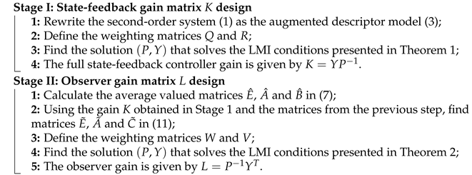
Actuators 13 00216 i001

4. Experimental Study

This section presents experimental studies to evaluate the proposed controller design methodology applied to balance the mobile inverted pendulum (MIP) robot in a vertical position (see Figure 1a). In the experiments, we applied the same control signal to the two robot motors. Notice that it is a non-linear and complex system with fewer actuators than degrees of freedom.
We used an MIP robot, which is an educational robotic kit developed at the University of California San Diego (UCSD) Coordinated Robotics Lab, available at Renaissance Robotics https://www.renaissancerobotics.com (accessed on 1 June 2024), as shown in Figure 1a. The MIP robot is controlled using a Beaglebone Black board attached with a robotics cape http://www.strawsondesign.com/#!board-features (accessed on 1 June 2024) which includes on-board sensors, controllers, and expansion options. The pyctrl library, available in [24], was used to implement the controllers at a sampling rate of 100 Hz.

4.1. System Model

A simplified MIP model depicted in Figure 1b was considered to obtain a model that characterizes the system. The body and the wheels were assumed to be rigid, and the sliding friction between the wheels and the ground was not considered.
The coordinates are x and y, θ is the body angle and ϕ the wheel angle, r represents the radius of the wheels, is the distance between the center of mass of the wheels ( C w ), and C b represents the center of mass of the body. Thus, one obtains the linearized, underactuated model as in (1) where:
M = a c b 2 0 0 a c b 2 , D = f ( a + b ) f ( a + b ) f ( b + c ) f ( b + c ) , S = a d 0 b d 0 , B = e ( a + b ) e ( b + c ) , z ( t ) = θ ( t ) ϕ ( t ) ,
and u ( t ) is the motor voltage, where a = r 2 ( m b + 2 m w ) + 2 I w , b = m b r , c = I b + m b 2 , d = m b g , e = 2 G r t m / V max , and f = 2 G r 2 C m . In addition, we assume w ( t ) a Gaussian zero mean white noise acting on both states, such that B w = [ 1 , 1 ] T × 10 6 . The parameters in the MIP model listed in Table 1 free of uncertainty are measurable or known physical specs. On the other hand, the unknown parameters were estimated using the MATLAB tfest function, whose fit to estimation data was approximately 96 % . The estimation procedure followed the same steps of Zhuo [25].
Note that because the second column of S in (25) is null, then ϕ ( t ) does not influence the other states. It makes sense since MIP can balance its body upright, no matter where the wheels are. One can check that the descriptor model (3) with data in (25) is controllable, but not observable. Therefore, we can design the observer-based controller removing the state ϕ ( t ) from the descriptor model obtained yielding x ( t ) = [ θ ( t ) θ ˙ ( t ) ϕ ˙ ( t ) ] T . In addition, in this case, we assume the system output as y ( t ) = [ θ ˙ ( t ) ϕ ˙ ( t ) ] T .
Here, to design the controllers, we take into account the uncertainty of ± 4 % on the values estimated from two experimental data sets to the parameters: I b , I w , t m , and C m . Because I b and I w were estimated from the same data set, we assume they simultaneously take their minimum or maximum estimated value. Analogously, the same is assumed for the values of t m and C m . Thus, we cast the descriptor system matrix as in (4) belonging to a polytope as in (5) with N = 4 vertices.
Finally, to validate the effectiveness and performance of the designed controllers in experimental tests we used the data acquired to compute the quantities { | θ | 2 , | θ ˙ | 2 , | ϕ | 2 , | ϕ ˙ | 2 } and { | u | 2 } related to the expectations.

4.2. Full State-Feedback Control

In this section, applying Theorem 1 are designed controllers based on full state feedback. Initially, we cast the uncertain descriptor model (3) as mentioned in the previous section, and we selected the weighting matrices as Q = I 4 and R = 1 , 2 , 5 . The choice of Q = I implies that each state is treated equally. Therefore, the resulting gains for the controllers are summarized in Table 2.

4.3. Observer-Based Control

Now, we design observer-based controllers. Thus, as discussed in Section 4.1, we eliminate the state ϕ ( t ) of the uncertain descriptor model (3) built before applying the proposed method. Without performing this elimination, the model is not observable, and Theorem 2 does not result in feasible results.
Following Stage 1 of the proposed approach to design the observer-based controller, we apply Theorem 1 setting the weighting matrices as Q = I 3 and R = 1 , 2 , 5 . The resulting gains for the controllers are summarized in Table 3.
Secondly, following Stage 2 of the method proposed, using the matrices K in Table 3, we apply Theorem 2 setting the weighting matrices as V = diag { 0.01 , 0.1 } and W F = [ E ^ 1 B ^ u 0 ] T . Table 4 summarizes the resulting gains for the controllers.

4.4. Experimental Results

In this section, the MIP time responses governed by the controllers designed previously are presented to illustrate the experimental results.
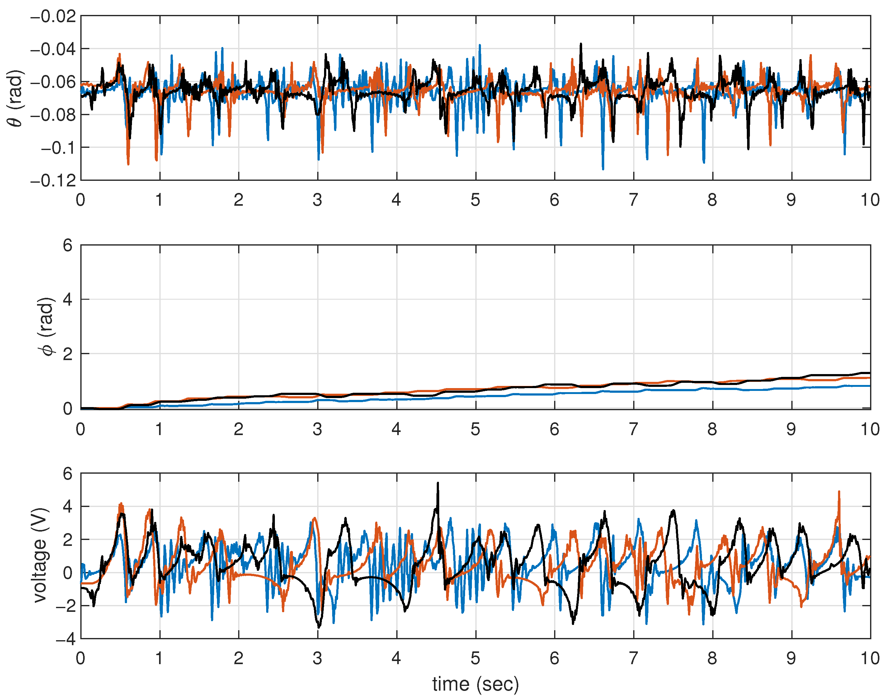
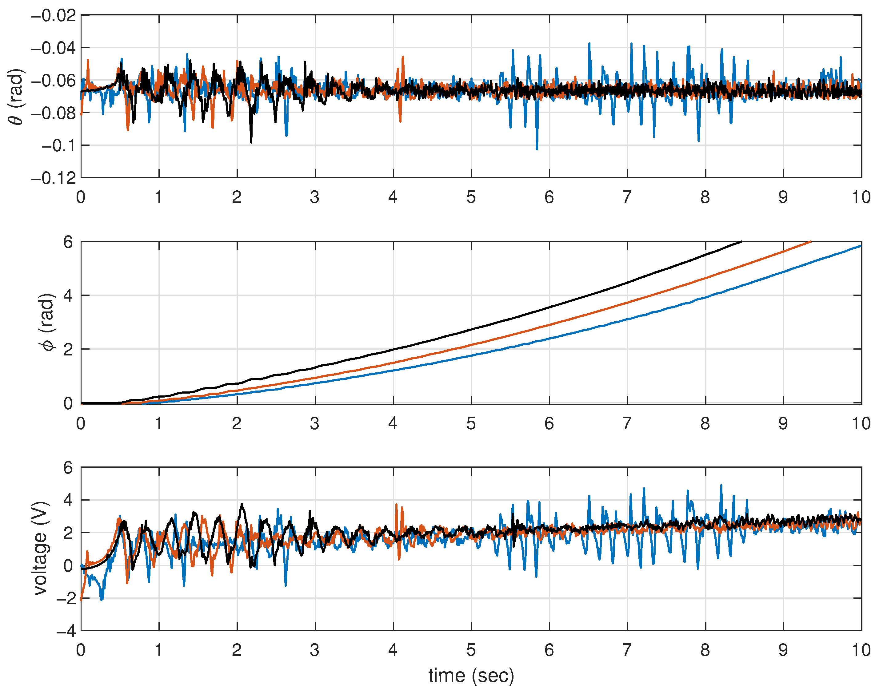
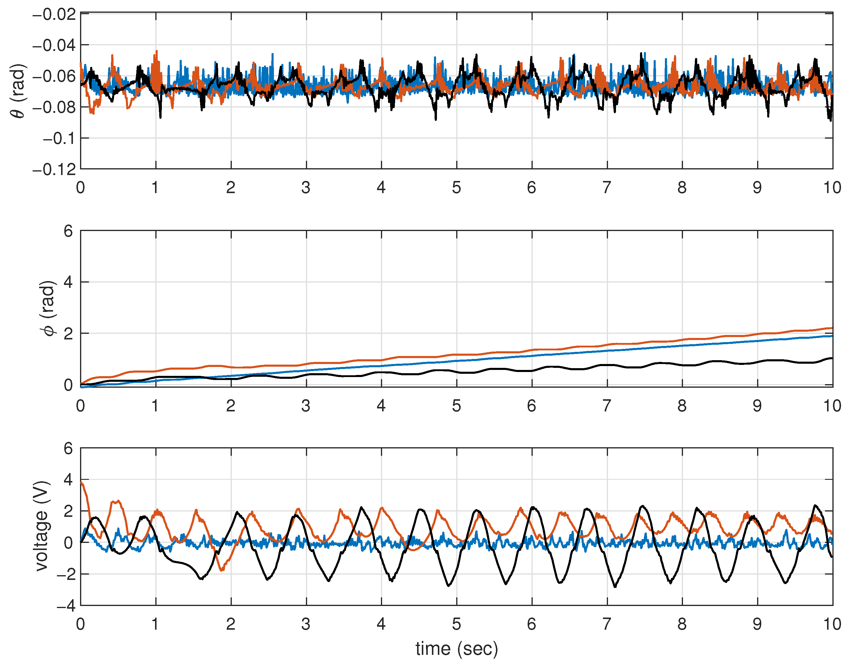
Initially, the time responses considering the controllers from Table 2 are depicted in Figure 2, where one can see that by increasing R, the MIP body oscillation decreases. Similarly, in Figure 3 are presented the time responses considering the controllers from Table 3.
It is interesting to note that the wheel angle deviation in Figure 3 is much higher than in Figure 2, which is comprehensible since the controllers applied to obtain the results depicted in Figure 3 do not use the wheel angle.
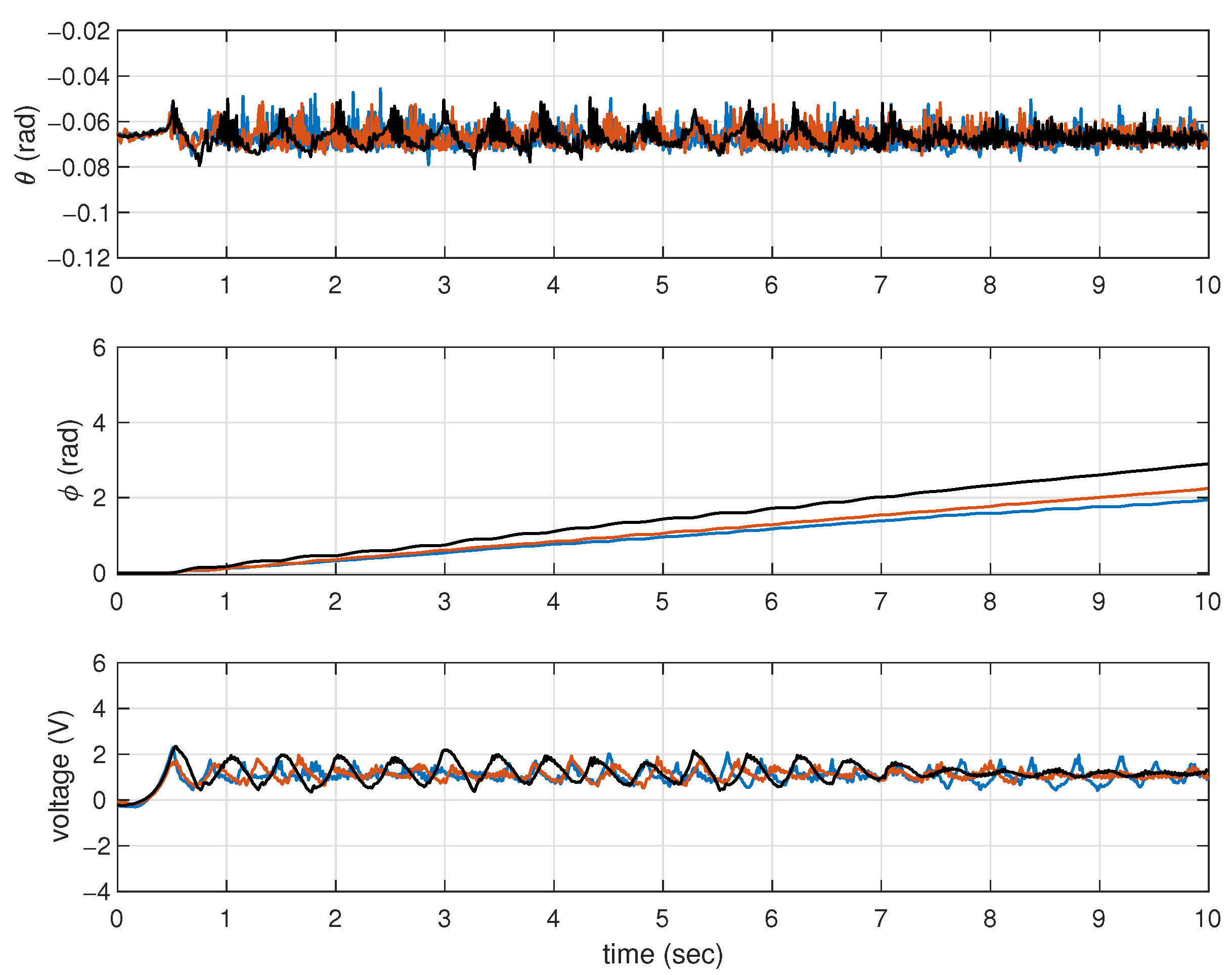
The time responses considering the observer-based controllers from Table 4 are depicted in Figure 4. Now, one can notice that body oscillations and control efforts have decreased. Furthermore, the deviation of the wheel angle in Figure 4 is smaller than that in Figure 3.
Finally, in Figure 5, we present the noises estimated on θ and ϕ obtained in the experiment with the full state feedback controller for R = 5 in Table 3. The noises were estimated by filtering θ and ϕ with 4th-order lowpass Butterworth filters with a cutoff frequency of 20 Hz and then subtracting the results from the respective unfiltered signals. Additionally, using the MATLAB cov function, the variances of the estimated noises on signals θ and ϕ were obtained which are given as σ θ 2 = 2.8606 × 10 5 and σ ϕ 2 = 5.6940 × 10 5 , respectively.
It is worth emphasizing that an exhaustive search on weighting matrices, Q, R, V, and W, the design parameters given in Theorems 1 and 2, may improve the controller performance.
Remark 1.
Despite the proposed method having been designed specifically for second-order dynamical systems, the approach applies to any dynamical system that can be cast in form (3). Hence, dynamic output-feedback controllers can be designed for a large class of systems without major assumptions on the characteristics of uncertainties (norm-bounded uncertainty, for instance).

4.5. Experimental Performance Comparisons

In this section, we briefly compare the experimental performance achieved by the controllers designed with the proposed methodology and some well-known similar methods from the literature, namely, ( i ) full state-feedback, robust H controller, and based on the nominal system model, ( i i ) linear–quadratic–Gaussian (LQG) controller, and ( i i i ) an observer-based controller combining a state-feedback LQR with an observer designed via eigenvalues placement.
Initially, taking into account the uncertain model with polytopic description, we design a full state-feedback, robust H controller following the method based on LMIs presented in [26], which yields the state-feedback control gains:
K = [ 7.7071 0.7965 0.4700 ] × 10 8 and γ = 1.0143 ,
where γ is the H guaranteed cost. Thus, as one would expect, this controller was not able to stabilize the MIP, because the control signal saturates very easily due to the controller’s high gains.
Further, considering the system nominal model, we design ( i ) a full state-feedback LQR for Q = I 3 and R = 1 , 2 , 5 , applying the MATLAB lqr function, where the control gains K obtained are listed in Table 5, and a ( i i ) linear quadratic estimator (LQE) using the MATLAB lqe function for V = diag { 0.01 , 0.1 } and W = diag { [ B ^ u T E ^ T E ^ 1 B ^ u , 0 } with resulting gain
L e = 1.5228 0.2696 611.6569 95.6262 956.2624 162.3013 .
Based on the data in Table 5, it is easy to see that the standard LQR is robust since the gains designed based on the system nominal model are very close to the ones designed based on the uncertain system model listed in Table 3. The data acquired in the experiments performed in the MIP governed by the standard LQRs are presented in Figure 6. Comparing Figure 3 and Figure 6, it is easy to note that the standard LQR designed with R = 1 resulted in a much more high-frequency oscillatory MIP dynamic than the proposed robust LQR designed with R = 1 .
It is worth recalling that in the proposed observed-based controller design (see Algorithm 1), an associated observer is designed for each state-feedback controller gain. On the other hand, in the classic methodology based on the system nominal model, the observer gains are designed independently of the state-feedback controller.
The data acquired in the experiments performed in the MIP governed by the standard LQGs, obtained by the combination of each K in Table 5 with the observer gains L e in (26), are presented in Figure 7. It can be seen that for the standard LQG designed with R = 5 , it resulted in high amplitude low-frequency oscillatory MIP dynamics, which for minor perturbations in the experiments culminated in an unstable response. The other results are similar to the ones present in Figure 4.
Despite the success obtained in the experiments applying the standard LQR and LQG controllers, it is worth mentioning that only the proposed robust controllers guarantee stability for the uncertain system model.
Finally, it is important to highlight that several attempts were made using the MATLAB place function to find suitable observer gains that combined with the controller gains in Table 5 could stabilize the system. However, in every tested scenario, the resulting observer-based controllers were ineffective in stabilizing the MIP.

5. Conclusions

In this paper, an approach was proposed to design dynamic output-feedback controllers for second-order linear dynamical systems. The formulated solution can tackle uncertainties in the model and persistent disturbances in the states using LMIs to minimize cost functions containing linear-quadratic criteria in a two-stage procedure. The approach is applied in experimental tests conducted in an MIP robot—an underactuated system—and effectively controls the body angle in an equilibrium position. Further research includes developing conditions involving other performance criteria, such as H -norm and finite-time stabilization, designing a one-step condition capable of simultaneously synthesizing the control and the observer gains, and extending the method to cope with nonlinear systems.

Author Contributions

Conceptualization, D.G. and F.d.O.S.; methodology, D.G., F.d.O.S. and J.M.A.; software, D.G. and F.d.O.S.; validation, D.G., F.d.O.S. and L.F.; formal analysis, D.G., J.M.A., L.F. and F.d.O.S.; investigation, D.G., J.M.A. and F.d.O.S.; resources, F.d.O.S.; data curation, F.d.O.S.; writing—original draft preparation, D.G., J.M.A., L.F. and F.d.O.S.; writing—review and editing, J.M.A., L.F. and F.d.O.S.; visualization, F.d.O.S.; supervision, F.d.O.S. and J.M.A.; project administration, F.d.O.S.; funding acquisition, F.d.O.S., J.M.A. and L.F. All authors have read and agreed to the published version of the manuscript.

Funding

This work was supported by the Coordination for the Improvement of Higher Education Personnel—Brazil (CAPES) through the Academic Excellence Program (PROEX), and by the National Council for Scientific and Technological Development (CNPq) under grants 306178/2023-0, 304606/2023-5 and 408419/2023-7.

Data Availability Statement

The data supporting this study’s findings are available from the corresponding author, J.M.A., upon reasonable request.

Conflicts of Interest

The authors declare no conflicts of interest.

References

  1. Ikeda, Y. Active and semi-active vibration control of buildings in Japan—Practical applications and verification. Struct. Control Health Monit. 2009, 16, 703–723. [Google Scholar] [CrossRef]
  2. Yu, Y.; Guo, J.; Li, L.; Song, G.; Li, P.; Ou, J. Experimental study of wireless structural vibration control considering different time delays. Smart Mater. Struct. 2015, 24, 045005. [Google Scholar] [CrossRef]
  3. Zhang, L.; Zhang, G.; Liu, W. Optimal control of second-order and high-order descriptor systems. Optim. Control Appl. Methods 2019, 40, 791–806. [Google Scholar] [CrossRef]
  4. Abdelaziz, T.H. Parametric approach for eigenstructure assignment in descriptor second-order systems via velocity-plus-acceleration feedback. J. Dyn. Syst. Meas. Control 2014, 136, 044505. [Google Scholar] [CrossRef]
  5. Luenberger, D.G. Observing the State of a Linear System. IEEE Trans. Mil. Electron. 1964, 8, 74–80. [Google Scholar] [CrossRef]
  6. Hayashi, S.; Kanoh, H.; Masubuchi, M. Functional Observers for Some Sort of Linear Systems and Its Application to Unstable Mechanical System. Technol. Rep. Osaka Univ. 1980, 30, 537–544. [Google Scholar]
  7. Trinh, H. Linear functional state observer for time-delay systems. Int. J. Control 1999, 72, 1642–1658. [Google Scholar] [CrossRef]
  8. Darouach, M. Existence and design of functional observers for linear systems. IEEE Trans. Autom. Control 2000, 45, 940–943. [Google Scholar] [CrossRef]
  9. Araujo, J.M.; Barros, P.R.; Dorea, C.E.T. Design of Observers with Error Limitation in Discrete-Time Descriptor Systems: A Case Study of a Hydraulic Tank System. IEEE Trans. Control Syst. Technol. 2012, 20, 1041–1047. [Google Scholar] [CrossRef]
  10. Trinh, H.; Fernando, T. Functional Observers for Dynamical Systems; Springer: Berlin/Heidelberg, Germany, 2012. [Google Scholar] [CrossRef]
  11. Darouach, M.; Fernando, T. On the Existence and Design of Functional Observers. IEEE Trans. Autom. Control 2020, 65, 2751–2759. [Google Scholar] [CrossRef]
  12. Ríos-Ruiz, C.; Osorio Gordillo, G.L.; Darouach, M.; Souley Ali, H.; Astorga-Zaragoza, C.M. Design of finite-time convergent functional observer for descriptor systems: Application to fault estimation. Asian J. Control. 2004. online first. [Google Scholar] [CrossRef]
  13. Demetriou, M.A. Natural second-order observers for second-order distributed parameter systems. Syst. Control Lett. 2004, 51, 225–234. [Google Scholar] [CrossRef]
  14. Demetriou, M.A. Unknown input functional observers for vector second order structural systems. Mech. Syst. Signal Process. 2022, 164, 108060. [Google Scholar] [CrossRef]
  15. Liu, Y.; Yu, H. A survey of underactuated mechanical systems. IET Control Theory Appl. 2013, 7, 921–935. [Google Scholar] [CrossRef]
  16. Seifried, R. Dynamics of Underactuated Multibody Systems: Modeling, Control and Optimal Design; Springer International Publishing: Cham, Switzerland, 2014. [Google Scholar] [CrossRef]
  17. Shin, J.H.; Lee, J.J. Fault detection and robust fault recovery control for robot manipulators with actuator failures. In Proceedings of the 1999 IEEE International Conference on Robotics and Automation (Cat. No.99CH36288C), Detroit, MI, USA, 10–15 May 1999. [Google Scholar] [CrossRef]
  18. Nudehi, S.S.; Mukherjee, R. Enhancing Controllability and Observability in Underactuated and Undersensed Systems Through Switching: Application to Vibration Control. J. Dyn. Syst. Meas. Control 2004, 126, 790–799. [Google Scholar] [CrossRef]
  19. Venkatraman, A.; Ortega, R.; Sarras, I.; van der Schaft, A. Control of underactuated mechanical systems: Observer design and position feedback stabilization. In Proceedings of the 2008 47th IEEE Conference on Decision and Control, Cancun, Mexico, 9–11 December 2008. [Google Scholar] [CrossRef]
  20. Gesser, R.S.; Lima, D.M.; Normey-Rico, J.E. Robust Model Predictive Control: Implementation Issues with Comparative Analysis. IFAC-PapersOnLine 2018, 51, 478–483. [Google Scholar] [CrossRef]
  21. Lin, K.J. Sliding Mode Control Design for Uncertain Singular Systems. Appl. Mech. Mater. 2012, 145, 16–20. [Google Scholar] [CrossRef]
  22. Zhong, Z.; Lam, H.K.; Ying, H.; Xu, G. CMAC-based SMC for uncertain descriptor systems using reachable set learning. IEEE Trans. Syst. Man Cybern. Syst. 2023, 54, 693–703. [Google Scholar] [CrossRef]
  23. Fairman, F.W. Linear Control Theory: State Space Approach; John Wiley & Sons: Chichester, UK, 1998. [Google Scholar]
  24. GitHub. Pyctrl: A Python Suite for Systems and Control. 2018. Available online: https://github.com/mcdeoliveira/pyctrl (accessed on 13 July 2023).
  25. Zhuo, Z. LQG Controller Design of the Mobile Inverted Pendulum. Master’s Thesis, University of California, San Diego, CA, USA, 2017. [Google Scholar]
  26. Gahinet, P.; Apkarian, P. A linear matrix inequality approach to H control. Int. J. Robust Nonlinear Control 1994, 4, 421–448. [Google Scholar] [CrossRef]
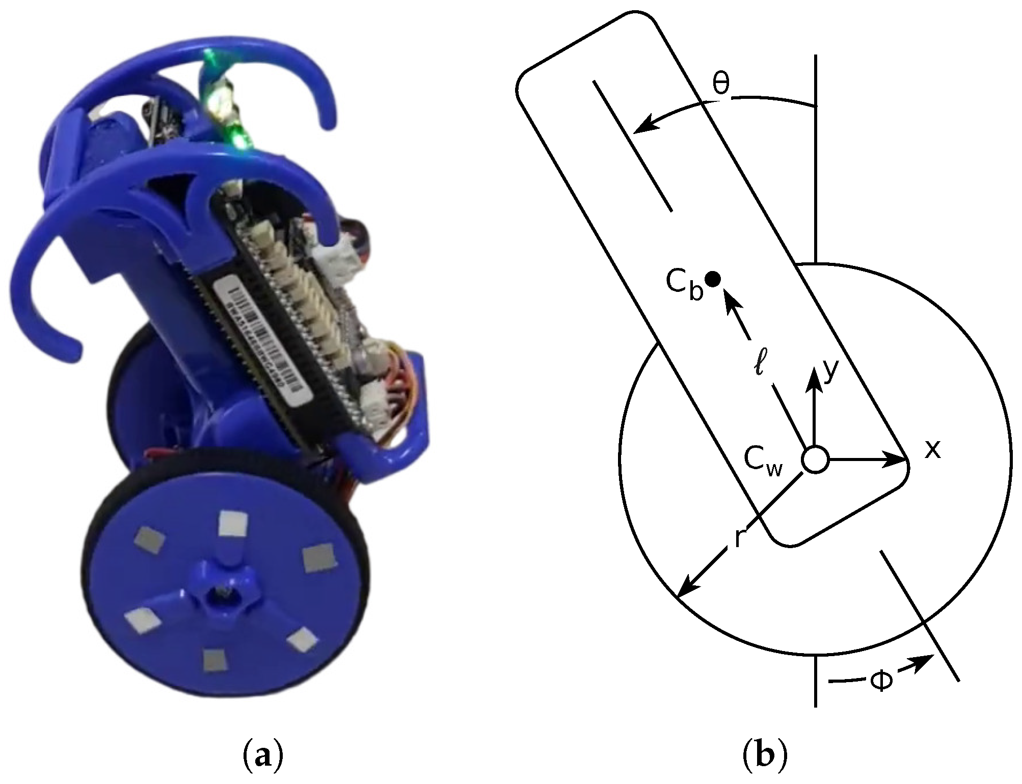
Figure 1. Mobile inverted pendulum robot: (a) Robot photo; (b) Robot sketch.
Actuators 13 00216 g001
Figure 2. Response of body position ( θ ), wheel angle ( ϕ ), and motor voltage (V), with full state-feedback controllers, for R = 1 , R = 2 and R = 5 , given in blue, red, and black lines, respectively. See Table 2.
Actuators 13 00216 g002
Figure 3. Response of body position ( θ ), wheel angle ( ϕ ), and motor voltage (V), with state-feedback controllers, for R = 1 , R = 2 and R = 5 , given in blue, red, and black lines, respectively. See Table 3.
Actuators 13 00216 g003
Figure 4. Response of body position ( θ ), wheel angle ( ϕ ), and motor voltage (V), with observer-based controllers, for R = 1 , R = 2 and R = 5 , given in blue, red, and black lines, respectively. See Table 4.
Actuators 13 00216 g004
Figure 5. Noises estimated on θ and ϕ data obtained in the experiment with the full state-feedback controller for R = 5 , with variances σ θ 2 = 2.8606 × 10 5 and σ ϕ 2 = 5.6940 × 10 5 , respectively.
Actuators 13 00216 g005
Figure 6. Response of body position ( θ ), wheel angle ( ϕ ), and motor voltage (V), with state-feedback controllers designed by the MATLAB lqr function for the nominal system model, with R = 1 , R = 2 and R = 5 , given in blue, red, and black lines, respectively. See Table 5.
Actuators 13 00216 g006
Figure 7. Response of body position ( θ ), wheel angle ( ϕ ), and motor voltage (V), with the LQG designed by MATLAB functions for the nominal system model, with R = 1 , R = 2 and R = 5 , given in blue, red, and black lines, respectively; and the observer gains L e in (26) designed with V = diag { 0.01 , 0.1 } and W = diag { [ B ^ u T E ^ T E ^ 1 B ^ u , 0 } . See Table 5.
Actuators 13 00216 g007
Table 1. The MIP parameters.
ParameterValueUncertaintyParameterValueUncertainty
r34 mm0 I b 4.98 × 10 4 kg·m2 ± 4 %
46 mm0 I w 6.13 × 10 5 kg·m2 ± 4 %
m w 27 g0 t m 0.0027 N·m at Vmax ± 4 %
m b 263 g0 C m 2.39 × 10 6 N·m ± 4 %
V max 7.4 V0 G r 35.57:1 Gear ratio0
Table 2. Full state-feedback controllers designed with Q = I 4 and R = 1 , 2 , 5 and the quantities { | θ | 2 , | θ ˙ | 2 , | ϕ | 2 , | ϕ ˙ | 2 } and { | u | 2 } computed with the data acquired in the experiments performed.
RK { | θ | 2 , | θ ˙ | 2 , | ϕ | 2 , | ϕ ˙ | 2 } { | u | 2 }
1 [ 27.7052 0.7149 2.7944 1.1473 ] { 0.0045 , 0.0081 , 0.2369 , 0.0637 } 1.6246
2 [ 23.6326 0.5724 2.3279 0.9844 ] { 0.0044 , 0.0086 , 0.5295 , 0.0948 } 1.5300
5 [ 19.0008 0.4020 1.7968 0.7967 ] { 0.0044 , 0.0114 , 0.5384 , 0.1571 } 2.1554
Table 3. State-feedback controllers designed with Q = I 3 and R = 1 , 2 , 5 and the quantities { | θ | 2 , | θ ˙ | 2 , | ϕ | 2 , | ϕ ˙ | 2 } and { | u | 2 } computed with the data acquired in the experiments performed.
RK { | θ | 2 , | θ ˙ | 2 , | ϕ | 2 , | ϕ ˙ | 2 } { | u | 2 }
1 [ 25.7311 2.5889 0.9951 ] { 0.0044 , 0.0054 , 7.5692 , 0.4613 } 3.7452
2 [ 21.8617 2.1416 0.8547 ] { 0.0044 , 0.0027 , 10.4583 , 0.5642 } 3.9529
5 [ 17.6030 1.6484 0.6984 ] { 0.0044 , 0.0044 , 14.9050 , 0.7364 }4.7545
Table 4. Observer gains designed with data in Table 3, V = diag { 0.01 , 0.1 } and W F = [ E ^ 1 B ^ u 0 ] T , and the quantities { | θ | 2 , | θ ˙ | 2 , | ϕ | 2 , | ϕ ˙ | 2 } and | u | 2 computed with the data acquired in the experiments performed.
RKL { | θ | 2 , | θ ˙ | 2 , | ϕ | 2 , | ϕ ˙ | 2 } { | u | 2 }
1 [ 25.7311 2.5889 0.9951 ] 1.6595 0.12703 684.05 10.488 1048.8 24.994 { 0.0045 , 0.0016 , 1.2520 , 0.0535 } 1.2038
2 [ 21.8617 2.1416 0.8547 ] 1.6162 0.12056 681.73 10.484 1048.4 24.469 { 0.0045 , 0.0014 , 1.5865 , 0.0664 } 1.2574
5 [ 17.6030 1.6484 0.6984 ] 1.5717 0.11392 679.54 10.485 1048.5 23.907 { 0.0045 , 0.0033 , 2.7282 , 0.1270 }  1.5946
Table 5. State-feedback controllers gains K designed by MATLAB lqr function with Q = I 3 and R = 1 , 2 , 5 ; and the quantities { | θ | 2 , | θ ˙ | 2 , | ϕ | 2 , | ϕ ˙ | 2 } and { | u | 2 } computed with the data acquired in the experiments performed with the LQR ( =  LQR) and the LQG controllers ( =  LQG), where the last controller results from the combination of the LQR gains in the table with the observer gains L e in (26) designed by MATLAB lqe function with V = diag { 0.01 , 0.1 } and W = diag { [ B ^ u T E ^ T E ^ 1 B ^ u , 0 } . All gains were designed considering the nominal model.
RK { | θ | 2 , | θ ˙ | 2 , | ϕ | 2 , | ϕ ˙ | 2 }
= LQR     = LQG
{ | u | 2 }
LQRLQG
1 34.3765 3.6098 1.2607 { 0.0056 , 0.0336 , 0.7557 , 0.1651 } L Q R
{ 0.0045 , 0.0012 , 1.1380 , 0.0509 } L Q G
7.15131.3807
2 26.0655 2.6461 0.9784 { 0.0045 , 0.0041 , 1.0429 , 0.2263 } L Q R
{ 0.0045 , 0.0052 , 1.7003 , 0.1329 } L Q G
2.55491.4242
5 19.1122 1.8388 0.7383 { 0.0044 , 0.0013 , 73.5951 , 2.6977 } L Q R
{ 0.0045 , 0.0097 , 0.3411 , 0.1818 } L Q G
13.02662.1356
Disclaimer/Publisher’s Note: The statements, opinions and data contained in all publications are solely those of the individual author(s) and contributor(s) and not of MDPI and/or the editor(s). MDPI and/or the editor(s) disclaim responsibility for any injury to people or property resulting from any ideas, methods, instructions or products referred to in the content.