Abstract
In this paper, the global stabilization problem of control systems with input saturation and multiple input delays is studied, and a new method is proposed to design nonlinear stabilization control laws. First, based on Luenberger’s canonical decomposition, the multiple-input delay system is transformed into a series of linear time-delay systems with single inputs and input saturation. However, for the converted system, each subsystem is coupled to the others. Therefore, the idea of recursion is adopted to construct a special state transformation with time delay for each subsystem and convert it into a linear system with time delay for both state variables and input variables. For the conversion system, a nonlinear controller with cascade saturation control is designed, and the controller includes some free parameters. The control performance of the controller is improved by adjusting the free parameters online. At the same time, a less conservative stability condition is established to ensure the dynamic performance of the closed-loop system. Finally, the effectiveness and superiority of the proposed method are verified by numerical simulation and practical applications in a spacecraft rendezvous system.
1. Introduction
Saturation nonlinearity is an inherent characteristic of most actuators in control systems. Once the actuator reaches its input saturation limit, any attempt to increase the output will yield no discernible change in the output, thereby limiting the dynamic performance of the system and potentially leading to instability. The presence of input saturation renders the system inherently nonlinear [1]. Therefore, like most nonlinear systems, the system with saturation nonlinearity presents a significant challenge to the design of nonlinear controllers. Consequently, the stabilization problem of control systems with input saturation has attracted widespread attention [2,3,4].
The stabilization of control systems with input saturation can be divided into three categories: global stabilization, semi-global stabilization, and local stabilization. The primary challenge in global stabilization is to design a controller that ensures the closed-loop system is not only stable but also has a domain of convergence that encompasses the entire state space. In 1995, Lin proposed an arbitrarily small and bounded-state feedback control law to globally stabilize nonlinear systems with input saturation based on Lyapunov analysis, LaSalle’s invariance principle, and center manifold theory. This method effectively addressed the global stabilization problem for multi-input multi-output nonlinear systems [5]. In [6], Yakoubi et al. further introduced a Lyapunov function and proposed a bounded state feedback control law with nested saturation to globally stabilize linear systems with input saturation and time delay. Additionally, they extended the proposed control law to the general case of arbitrarily small bounds on the controller, as discussed in [5]. Zhou et al. [7] combined the gain scheduling approach with a low-gain feedback design method based on the Lyapunov equation to propose a novel global stabilization control law. This method offers the advantage of not involving nonlinear optimization problems or requiring the online solving of the algebraic Riccati equation (ARE), as all design parameters are predetermined. On this basis, Zhou et al. [8] further extended the above ideas to time-delay systems, and established the feedback control law of low-gain feedback design based on parameterized Lyapunov equation.
On the other hand, due to the delay in feedback control actions, the limitations of measurement tools, and simplifications in dynamic model descriptions, time-delay phenomena are widely present in many dynamic systems in real life. It is noteworthy that time-delay phenomena can cause various issues, such as system instability, divergent system states, and oscillations in dynamic systems.
Consequently, over the past few decades, the study of time-delay systems, particularly in the areas of asymptotic stability analysis and stabilization, has garnered extensive attention [9,10,11].
There are many methods to address the asymptotic stability and stabilization of time-delay systems, with the most effective ones possibly being those based on the Lyapunov–Krasovskii functional method [12] and the Razumikhin theorem. The idea is to find a positive definite functional whose derivative along the system trajectory is negative, converting the result into linear matrix inequalities for numerical solving. However, these methods typically provide conservative sufficient conditions, with complex criteria and heavy computational burdens.
Another effective method for handling time-delay systems is predictor feedback [13]. In [14], Manitius et al. proposed a new method that uses the current state and past control signals to predict the future state, thereby compensating for input delays. The controller includes integral terms of past control signals, making it infinite-dimensional, but the closed-loop system has only a finite number of zeros. Krstic et al. [15] utilized a novel concept, viewing input delay as a hyperbolic partial differential equation, to propose a predictive boundary control method based on backstepping transformation. A significant advantage of this method is its straightforward construction for the infinite-dimensional transformation of actuator states, thereby achieving a tightly integrated system between the transformed stable actuator dynamics and the controlled object dynamics. However, while almost all existing studies primarily address cases with constant time delays, variable time delays receive insufficient attention.
Recently, control strategies for delay systems based on predictors have regained widespread interest. For instance, Krstic et al. established the exponential stability of linear systems with distributed actuator delay and based on predictor feedback by using the Lyapunov functional in [16]. However, the controllers established by the above methods all contain integral terms, and it is very difficult to realize them in practice. Therefore, Zhou et al. [17] proposed a truncated predictor feedback method, safely removing the integral terms in cases where the open-loop system is only polynomially unstable. This method focuses solely on compensating for input delays. Specifically, if a controller is designed for a linear system with only state delays, then for an open-loop system with additional input delays, a compensator will be designed to ensure that the closed-loop system remains asymptotically stable. However, removing the integral terms inevitably affects the system’s dynamic performance. In previous studies, although Krstic and Zhou made progress in controlling linear systems with time delays, their methods have limitations in practical applications, especially in controlling dynamic performance. In response to these limitations, Zhang et al. [18] proposed a new stabilization method for linear time-delay systems. By innovatively designing regional stability and stabilization control strategies, they not only effectively controlled the distribution area of system eigenvalues but also precisely adjusted the system’s dynamic performance, such as response speed and damping ratio. This method particularly emphasizes control accuracy in handling non-connected regions, overcoming the dynamic performance loss caused by previous methods’ neglect of distributed items, demonstrating its broad application prospects in theoretical research and engineering practice.
On the other hand, over the past few decades, the control of linear systems with time delay, especially input time delay, has also received extensive attention. Many researchers have considered the control problem of systems with saturation and time delay [19,20,21]. In [21], Mazenc et al. proposed that an integral chain with arbitrarily large input delays can be stabilized through saturated feedback and established a nested saturated-type nonlinear controller. Then, in [6], Yakoubi et al. further extended these results to a class of zero-controllable systems controlled by bounded controllers. For oscillatory systems with input saturation and time delays, Fang et al. proposed a linear controller that can globally stabilize systems with arbitrarily large delays [22].
However, for general asymptotically zero-controllable systems with input saturation and time delays, particularly those with repeated poles on the imaginary axis, only semi-global stabilization is achievable. Therefore, Zhou et al. [8], based on a low-gain feedback design method from parametrized Lyapunov equations, established a new feedback control law and provided explicit conditions to ensure the stability of the closed-loop system, achieving global stabilization by adjusting the low-gain parameter online. Subsequently, Zhou et al. [23] further extended their results to discrete systems by exploring some complex properties of the low-gain feedback design method from parametric Lyapunov equations, thereby establishing both state feedback and output feedback control laws. This new method not only has a simple structure but also provides clear conditions to ensure the stability of the closed-loop system.
In 2013, Zhou et al. [24] further developed the truncated predictive feedback approach, constructing a state feedback control law that uses only the current state of the system, where the feedback gain depends on the delay information of the open-loop system and is hence referred to as delay-dependent feedback. This method provided precise conditions for determining the asymptotic stability of the closed-loop system, and if the delays in the system are time-varying or even unknown, a modified delay-independent truncated predictive feedback was established to address the stabilization issue.
In the stability analysis of dynamic systems, considering delays is crucial. Recently, researchers have devoted significant efforts to developing delay-dependent and delay-independent conditions to ensure system trajectory stability. For instance, in [25], Song et al. pioneered the use of delay partitioning and Lyapunov–Razumikhin function methods to establish conditions that ensure all trajectories of the resulting closed-loop system converge to the vicinity of the equilibrium point. However, these conditions are somewhat conservative and are not generally applicable to delay systems with actuator saturation. Building upon this foundation, T. Saravanakumar significantly advanced the control performance for Semi-Markovian Jump Linear Parameter Varying (S-MJLPV) systems under actuator saturation and faults [26]. This paper proposed a novel transformed parameter-dependent control method that not only achieves stochastic stability but also maintains an performance index despite the presence of actuator saturation and faults. Utilizing a mode-dependent Lyapunov function, Saravanakumar derived new sufficient conditions that are less conservative and more applicable to a broader range of systems, ensuring the stochastic stability of S-MJLPV systems.
In this paper, the global stabilization problem of control systems with input saturation and multiple input delays is studied in depth. A new cascade saturation control strategy is proposed for continuous linear systems with input saturation and multiple input delays, which are transformed into a series of single-input linear delay systems. Based on the recursive design idea, a special state transition strategy is constructed, a global stabilization control law is designed, and clear stability conditions are established. Compared with existing methods, the main contributions of this paper are as follows:
- (1)
- The multi-input time-delay system is adeptly transformed into a series of single-input linear time-delay systems. By engineering a state transformation that incorporates time delays, the state elimination characteristic previously identified in [27] is effectively extended to scenarios involving time delays, thus offering a novel and robust approach to addressing the challenges associated with time delays.
- (2)
- The designed controller not only makes full use of the current and lagging state information of the system but also significantly improves the dynamic performance of the closed-loop system through the cascade saturation control strategy. At the same time, the resource utilization and calculation efficiency are optimized, the design and implementation process is simplified, and the stability and efficiency of the system are ensured.
- (3)
- Free parameters that can be adjusted online are introduced, so that the controller can flexibly adjust its parameters according to real-time feedback to adapt to the changes in the dynamic characteristics of the system. This mechanism enhances the adaptability and stability of the system and allows more detailed control performance adjustment.
The rest of this paper is organized as follows. The problem formulation and preliminaries are presented in Section 2. The controller design of this paper is given in Section 3. In Section 4, two numerical simulations, namely a theoretical simulation and a control simulation, of a spacecraft rendezvous system are given to illustrate the effectiveness and superiority of the proposed method. Section 5 concludes this paper.
2. Problem Formulation
In this paper, the symbol denotes the n-dimensional Euclidean space, represents the set of all real matrices; I denotes the identity matrix; represents the set , denotes the saturation function, i.e., , where , and is denoted as when ; represents the Euclidean norm of a vector or the 2-norm of a matrix; denotes the controllability matrix of , where . denotes the inverse and transpose of matrix A, and represents the diagonal matrix composed of elements . denotes the Laplace transform of the state and input in the continuous case.
Consider a continuous linear system with input saturation and multiple input delays as follows:
where is a known constant and and are the state vector and control input, respectively. Here, represents the actuator saturation function, i.e., , and each saturation function is . is a system matrix with , and is any given input matrix. It is assumed that the matrix pair is controllable. The form of the controller is as follows:
where is a linear function of , and the resulting closed-loop system is as follows:
The problem addressed in this paper is as follows:
Problem 1.
Before designing the controller, we first present relevant lemmas, which are crucial to the main results established in this paper.
Lemma 1
([28]). Consider the following two time-delay systems:
where , and A is a nilpotent system matrix and τ represents the system’s delay time. The forms of and are as follows:
where is a set of given positive constants. Then, there exists a non-singular transformation
such that it converts system (4) into system (5). Here, and are the Laplace transforms of and , respectively, and is a matrix polynomial with the following form:
where .
Remark 1.
In order to better analyze the stability of the closed-loop control system in this paper, the above lemma can transform a linear system with only input delay into a linear system with both input delay and state delay.
Lemma 2
([29]). Consider the following linear system:
where the matrix pair is controllable. Consequently, there exists a non-singular matrix such that , which converts the system (8) into the following form:
where and are of the following form, respectively:
Remark 2.
The above lemma transforms a multi-input time-delay system into a series of linear time-delay systems each with a single-input form based on Luenberger’s canonical decomposition, where ‘*’ in the above formula represents possible non-zero elements.
3. Main Results
This section will make full use of the current and lagged state information of the system to propose a new method to address the aforementioned issues. For this purpose, we first transform system (1) into a series of single-input linear time-delay systems with input saturation by utilizing Lemma 2. Then, by constructing a special state transformation and employing recursive thinking, we design a global stabilization control law and establish explicit stability conditions.
Now, consider the time-delay system (1) and assume that the matrix pair is controllable. According to Lemma 2, there is a non-singular transformation that transforms the multi-input time-delay system (1) into the following form:
in which the forms of and are as follows:
where takes the following form:
Here, the symbol ‘*’ represents possible non-zero elements and .
Remark 3.
Let ; then, the form of the transformation matrix is as follows:
Let the controller . Therefore, the system (10) can be further written as
From system (11), it can be seen that each subsystem is coupled with others. For each subsystem controller, it is not required to be the global stabilizing controller for the entire system. To address this issue, a recursive design approach will be adopted to design the global stabilizing controller.
First of all, let be a series of given positive constants and . Then, consider the time-delay system (11) and the system with input saturation
where the forms of and are as follows:
and
According to Lemma 1, there exists a transformation , which is
such that the time-delay system (11) is transformed into the system (12).
Remark 4.
In the time domain, Equation (14) can be expressed as
where . Therefore, if the controller can stabilize system (12), then the same controller can also stabilize system (11). Moreover, Equation (15) reveals that contains both the current and lagged information of . Thus, for system (11), is achievable.
Based on the above analysis, the main results of this section are given. Firstly, the design of the l-th controller is introduced.
According to Theorem 1 from the literature [28], let , be a series of given positive numbers satisfying
and then the controller ; that is,
where is some scalar that satisfies , and the following inequality:
Similar to the analysis of Theorem 1 in the literature [28], if Equation (19) holds, there exists a finite time such that for all , the controller (18) can be expressed as
Thus, the closed-loop system, consisting of systems (16) and (20), is as follows:
Therefore, the closed-loop system (21) is asymptotically stable when Equation (17) holds.
Now, let us design the controller , where .
Theorem 1.
Let be a series of given positive constants satisfying
Then, the controller ; that is,
where is some scalar satisfying and
Proof of Theorem 1.
Consider the -th order subsystem in system (12) as follows:
From the -th order subsystem (16), it is clear that under the controller . Therefore, through Equation (15), as , we have
For system (25), consider the -th order subsystem as follows:
where . Then, integrating from to t on both sides of the system (26), we obtain
Therefore, we have
By substituting Equation (28) into Equation (26), we obtain
where .
Since , there is a finite time , which makes hold. Therefore, from the system (23), we can obtain
Therefore, we have
According to [28], if holds, that is, Equation (24) holds when , then there is a finite time to satisfy the following equation:
Therefore, according to Equation (25), we obtain
Thus, system (25) can be further simplified as
Now, consider the -th subsystem of the system (34), namely
Since , there exists a finite time such that
Repeating the above steps, we have
That is, Equation (24) holds when . Then, there exists a finite time such that it satisfies
Next, repeating the above steps, it is known that there exists a finite time such that for all , it holds that
where has the following form
Thus, system (38) is asymptotically stable if and only if , is asymptotically stable. It follows from the design of the controller that the system , is asymptotically stable if and only if holds. Finally, the overall process is repeated in order to design the controller . This completes the proof. □
Remark 5.
For the simplified closed-loop system (38), the system matrix is in the form of a lower triangle, so the characteristic equation of the system is as follows:
Then, we can obtain , . Thus, system stabilization is ensured when all these eigenvalues lie in the left half plane of the complex plane.
Remark 6.
According to Lemma 1, system (11) is transformed into (12). Comparing the two systems, it is evident that system (12) appears more complex since it includes time delays in both the input and the state variables. However, as demonstrated in the proof of Theorem 1, the state delays in system (12) can be sequentially eliminated through feedback, resulting in a lower triangular form for the final closed-loop system. This makes it easier to analyze the stability of the system. This explains why system (11) is transformed into the specific form of system (12).
Remark 7.
Based on the analysis results presented in this paper, the transformation between system models is independent of the delay τ. Therefore, our approach can be further extended to linear systems with time-varying delays, where the delay is bounded and satisfies Lemma 5 in [30], thereby enabling the design of corresponding globally stabilizing controllers. Specifically, by integrating recursive design with cascade saturation control strategies, we can not only achieve global stabilization in fixed-delay scenarios but also ensure the robustness and stability of the system in time-varying delay scenarios. Hence, our research provides a new and effective pathway for global stabilization control in systems with time-varying delays.
4. Numerical Examples
In this paper, we will conduct two critical simulation experiments to validate the control system theory we have developed. The first experiment, a theoretical simulation, aims at thoroughly exploring the fundamental principles of the theory. The second experiment tests the theory in a specific real-world scenario: the rendezvous system of a circular spacecraft. Together, these experiments not only solidify the foundation of our theoretical analysis but also significantly demonstrate the practical applicability of our theory in real-world systems.
4.1. Simulation Analysis of State Feedback Control
In this section, we validate the theory of global stabilization for control systems with input saturation and multiple input delays. Through carefully designed simulations, we demonstrate how global stabilization can be achieved using recursive design and cascade saturation control with nonlinear controllers in the presence of system noise. This part of the simulation experiment not only verifies the effectiveness of the control theory but also lays the foundation for subsequent practical application simulations.
Consider a fifth-order system with input saturation and multiple input time delays as follows:
where s, A and B are as follows:
From the above, the rank of the controllability matrix is 5, meaning that the system is controllable. Therefore, the above theory is applied to design a stabilizing controller for the system (40). The system (40) is converted into the following form:
where and are as follows:
The system (41) is then transformed into the following form:
where and are as follows
First, for the second subsystem of system (42), the controller is designed to satisfy . Then, let , , where . Let , where .
Next, the controller is designed for the first subsystem of system (42) to satisfy . Then, let
where . Let , where . The initial conditions of the system are chosen as , the system noise .
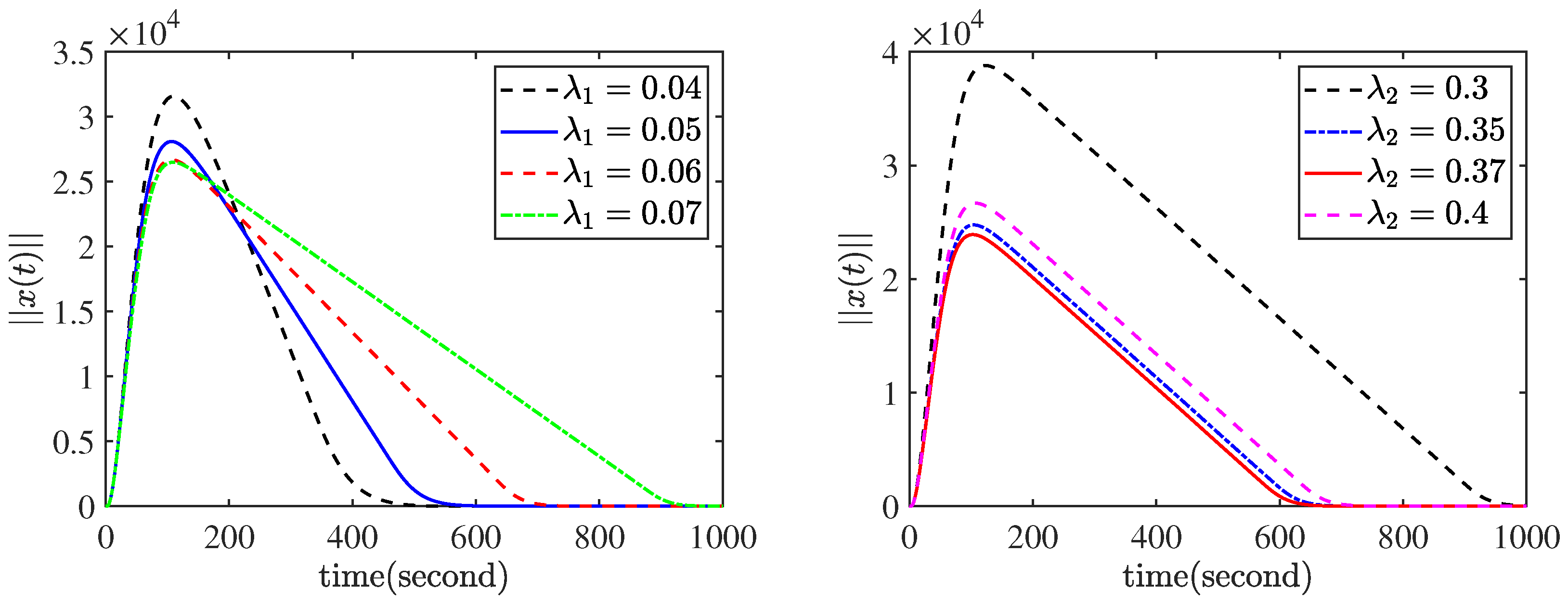
Finally, consider the impact of parameters and on the performance of the closed-loop system. Under controllers (18) and (23), the effects of different values of parameters and on the performance of the closed-loop system are shown in Figure 1. It can be seen that the dynamic performance of the closed-loop system varies with different values of and , and the designed controller achieves the best control performance when the parameters are and .
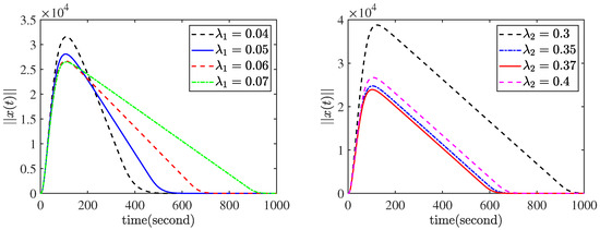
Figure 1.
The dynamic response of the closed-loop system under different and .
In order to illustrate the effectiveness and superiority of the control scheme proposed in this paper, we will compare it with the control schemes proposed in [31,32]; the truncated predictive feedback controller with input saturation, as described in [31], is chosen as follows:
where is the unique positive definite solution of the following equation.
After simulation, we can obtain . Then, using the dde-biftool toolbox in Matlab, the form of is calculated as follows:
The nested saturation controller described in [32] is as follows:
where
in which are a series of scalars satisfying
and
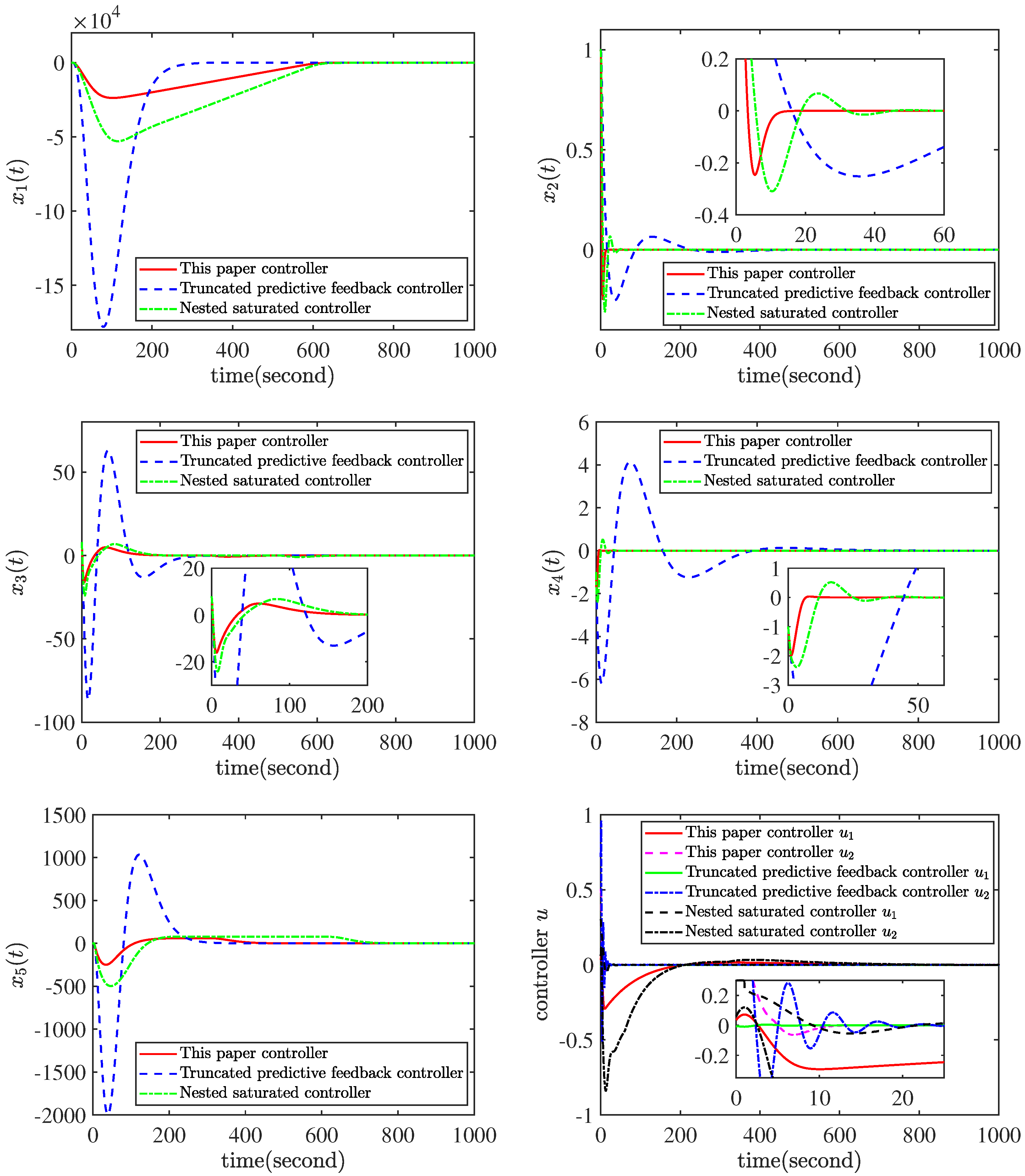
The same initial conditions were selected for the simulation. For the method proposed in [32], we first design the controller for system (42) such that satisfies . Let , where . Let with . Then, we design the controller such that satisfies . Let , where and with . Finally, the simulation results show that the parameters and have the best control performance. The resulting figures are presented in Figure 2. It is evident that the controller designed in this paper shows superior control performance in comparison to the truncated predictive feedback controller [31] and the nested saturation controller [32]. As can be seen from Figure 2, the system state has good regional stability under the controller with input saturation in the presence of system noise.
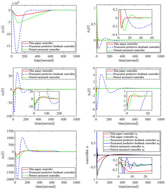
Figure 2.
The comparison of state trajectories of closed-loop systems with three controllers and control inputs.
Remark 8.
The nonlinear control method proposed in this paper effectively meets the challenges of input saturation and multi-input time delay through recursive design and cascade saturation control laws, and significantly improves the dynamic performance of the system. This method allows the performance to be optimized by adjusting the parameters of the controller online and makes full use of the current and lagging state information of the system, thus enhancing the ability to predict and adjust the system behavior. Through special state transition and recursive design, a clear global stabilization control law and explicit stability conditions are established.
In contrast, the truncated predictive feedback controller [31] (TPF) removes the integral term to simplify the control law, reducing the computational complexity, but also harming the dynamic response and performance of the system, especially in situations that require accurate or fast response.
Compared with cascade saturation controller, the nested saturation controller (48) [32] can provide strong robustness, but it also has obvious shortcomings. Firstly, because of the complexity of its internal structure, which involves a multi-layer saturation function, a nested saturation controller will slow down the response speed of the system. Secondly, the parameter adjustment of nested saturation controller is more complicated, especially when there are many layers in the control system, the saturation restrictions of each layer influence each other, which makes the system tuning more difficult. Generally speaking, the control strategy proposed in this paper shows superior performance and application potential in both theory and practical applications.
4.2. Simulation of a Rendezvous System of Circular Spacecraft
This section applies the theory developed in this paper to address the global stabilization problem of a circular spacecraft rendezvous system with input saturation and multiple input delays. The model is initially simplified by the introduction of new variables, followed by a model transformation that converts the simplified system model into a state-space representation. Subsequently, the final transformed system model undergoes controller design and simulation verification.
The spacecraft rendezvous system model, as illustrated in Figure 3, is worthy of consideration. First, consider a target spacecraft in a circular orbit with a radius of R, with a gravitational parameter of , where M is the mass of the central planet and G is the gravitational constant. represents the orbital rate of the target orbit. The relative motion between the target and the chaser (in the right-handed coordinate system, i.e., the rotating coordinate system) can be derived from Newton’s equations [33], specifically,
where , and denote the relative movement distance of spacecraft during rendezvous and docking and the acceleration due to the thrust of the tracker, respectively. Consequently, the linearized equations are provided in [33] as follows:
Furthermore, when , the system (50) is known as the Hill equation or the Clohessy–Wiltshire equation.
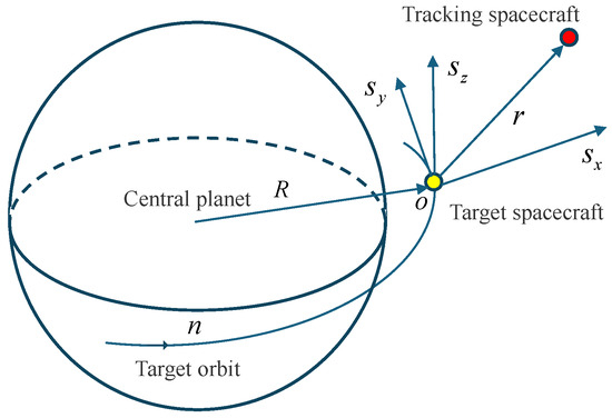
Figure 3.
The model of the spacecraft rendezvous system.
It is established from system (50) that the in-plane motion encompasses variables and , the out-of-plane motion comprises variable , and the variables and are not coupled to each other. Furthermore, the out-of-plane motion can be described as a simple oscillator, which is an asymptotically zero-controllable system. In the following form, the state variable is designated as x and the control input as u:
Then the state space equation for motion in the plane is as follows:
The system (52) with input delay can be written as follows:
where A and B are two constant matrices as follows:
It is easy to see from the above equation that the matrix pair is controllable. Meanwhile, the whole rendezvous process can be described by the transformation of the state vector from the nonzero initial state to the final state , where is the rendezvous time.
Now, we consider system (53) and design a nonlinear controller satisfying to make the closed-loop system globally asymptotically stable, where and are given positive constants, indicating the maximum acceleration generated by the thrust in two directions. Next, the design of the controller is divided into the following steps:
Step 1: According to Lemma 2, the system (53) is transformed into Luenberger’s canonical form. Let , and the non-singular transformation that is chosen has the following form
Consider the transformation , where . Thus, the following state equation can be obtained:
where , and and are given by
in which and . From system (56), we can obtain
where and are given by
Step 2: According to the theory of this paper, consider the following time-delay systems
where and take the following form
Then, there exists an invertible transformation
such that system (58) is transformed into system (59).
Step 3: For the time-delay system (59), according to the results of this paper, the nonlinear cascade saturation controller for this system is given as follows:
where and are a series of given positive constants that satisfy Equation (19), and and ε are a series of scalars that satisfy Equation (24).
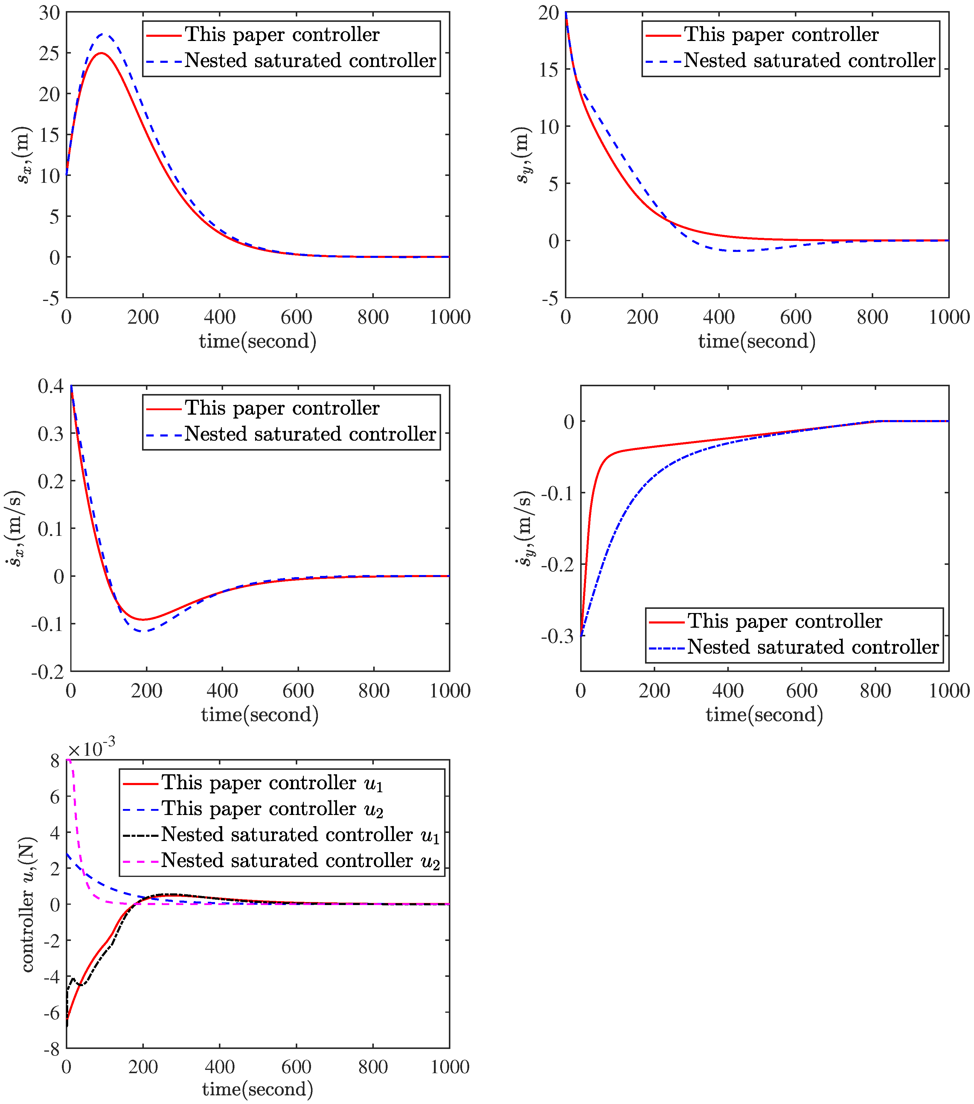
Unlike the controller design, the simulation will be carried out directly on the nonlinear model (49). Assume that the target spacecraft is in a circular orbit around the Earth, with an orbital height of 500 km. Therefore, the radius of the target orbit is m and the gravitational parameter is . Let m/s2, m/s2 and the delay time s. Therefore, the parameters of the nonlinear controller (61) are , m/s2, , , with . For simulation purposes, the initial condition is chosen to be . the system noise .
In order to show the effectiveness and superiority of the method proposed in this paper in the actual system, we choose to compare it with the nested saturation controller (45) in [32], and the same initial conditions were selected for the simulation. We first design the controller for system (59) such that satisfies m/s2. Let , with . Then, we design the controller such that satisfies m/s2. Let , where and with . Finally, the simulation results show that the parameters and have the best control performance. The simulation results are shown in Figure 4.
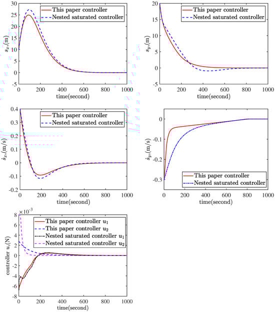
Figure 4.
The state trajectories of the circular spacecraft rendezvous system and control inputs.
Since the tracker and the target spacecraft are in relative motion with each other, it can be seen from Figure 4 that the relative motion of the tracker and the target spacecraft is zero in a finite time under the controller (61), that is, the two spacecraft achieve the rendezvous, which further verifies the practicability of the theory established in this paper. From Figure 4, it can be known that the method proposed in this paper is superior to the nested saturation type controller in the application of real system [32].
5. Conclusions
In this paper, an innovative design method for a stabilization control law is proposed for continuous control systems with input saturation and multiple input delays. Firstly, the original system is transformed into a series of single-input linear systems, all of which have input saturation characteristics, but it is worth noting that these subsystems are coupled with each other. In view of this structure, the controller of each subsystem does not have to be a global stabilization controller for the whole system. On this basis, this paper adopts a recursive strategy to construct an upper triangular state transformation with a time delay for each subsystem, which introduces a time delay in both state and input variables. On this basis, a nonlinear control law with cascade saturation control is designed for the transformed system, and the explicit stability conditions are clearly established. Finally, to verify the practical application value and theoretical correctness of the proposed method, it is validated by theoretical simulation, and the theoretical results are applied to the rendezvous system for circular spacecraft. The simulation results not only prove the effectiveness of the control strategy but also show its advantages in dealing with complex dynamic systems. The simulation results show that, compared with the traditional methods, the control strategy in this paper can greatly improve the dynamic performance of the system while ensuring its stability.
Author Contributions
Conceptualization, B.L.; Methodology, J.W., J.L., M.L. and B.Y.; Formal Analysis, J.W., B.L., J.L., M.L. and B.Y.; Data Curation, J.W.; Writing—Original Draft Preparation, J.W.; Writing—Review and Editing, J.W., B.L., J.L., M.L. and B.Y.; Visualization, J.W.; Supervision, B.L.; Project Administration, B.L.; Funding Acquisition, B.L. All authors have read and agreed to the published version of the manuscript.
Funding
This study was funded by the Fundamental Strengthening Program Technical Field Fund, Grant/Award Number: 2021-JCJQ-JJ-0026.
Institutional Review Board Statement
Not applicable.
Informed Consent Statement
Not applicable.
Data Availability Statement
The original contributions presented in the study are included in the article, further inquiries can be directed to the corresponding author.
Conflicts of Interest
The authors declare no conflicts of interest.
References
- Zhou, B.; Zheng, W.; Duan, G. An improved treatment of saturation nonlinearity with its application to control of systems subject to nested saturation. Automatica 2011, 47, 306–315. [Google Scholar] [CrossRef]
- Luo, W.; Zhou, B.; He, L. Global stabilization of the spacecraft rendezvous system by delayed and bounded linear feedback. IEEE Trans. Syst. Man Cybern. Syst. 2020, 52, 1373–1384. [Google Scholar] [CrossRef]
- Yang, X.; Zhou, B.; Mazenc, F. Global stabilization of discrete-time linear systems subject to input saturation and time delay. IEEE Trans. Autom. Control 2020, 66, 1345–1352. [Google Scholar] [CrossRef]
- Qin, J.; Du, J.; Li, J. Adaptive finite-time trajectory tracking event-triggered control scheme for underactuated surface vessels subject to input saturation. IEEE Trans. Intell. Transp. Syst. 2023, 24, 8809–8819. [Google Scholar] [CrossRef]
- Lin, W. Input saturation and global stabilization of nonlinear systems via state and output feedback. IEEE Trans. Autom. Control 1995, 40, 776–782. [Google Scholar] [CrossRef]
- Yakoubi, K.; Chitour, Y. Linear systems subject to input saturation and time delay: Global asymptotic stabilization. IEEE Trans. Autom. Control 2007, 52, 874–879. [Google Scholar] [CrossRef]
- Zhou, B.; Lin, Z.; Duan, G. Robust global stabilization of linear systems with input saturation via gain scheduling. Int. J. Robust Nonlinear Control IFAC-Affil. J. 2010, 20, 424–447. [Google Scholar]
- Zhou, B.; Lin, Z.; Duan, G. Stabilization of linear systems with input delay and saturation-A parametric Lyapunov equation approach. Int. J. Robust Nonlinear Control IFAC-Affil. J. 2010, 20, 1502–1519. [Google Scholar]
- Yang, X.; Zhou, B. Bounded controls for discrete-time linear systems subject to input time delay. J. Frankl. Inst. 2022, 359, 4893–4914. [Google Scholar] [CrossRef]
- Duan, Z.; Kong, L.; Fan, D.; Zhang, X. Adaptive tracking control of uncertain large-scale nonlinear time-delay systems with input saturation. Int. J. Syst. Sci. 2021, 52, 3254–3265. [Google Scholar] [CrossRef]
- Niu, X.; Lin, W.; Gao, X. Static output feedback control of a chain of integrators with input constraints using multiple saturations and delays. Automatica 2021, 125, 109457. [Google Scholar] [CrossRef]
- Pepe, P.; Jiang, Z.; Fridman, E. A new Lyapunov–Krasovskii methodology for coupled delay differential difference equations. Int. J. Control 2008, 81, 107–115. [Google Scholar] [CrossRef]
- Krstic, M. Compensation of infinite-dimensional actuator and sensor dynamics. IEEE Control Syst. Mag. 2010, 30, 22–41. [Google Scholar]
- Manitius, A.; Olbrot, A. Finite spectrum assignment problem for systems with delays. IEEE Trans. Autom. Control 1979, 24, 541–552. [Google Scholar] [CrossRef]
- Krstic, M.; Smyshlyaev, A. Backstepping boundary control for first-order hyperbolic PDEs and application to systems with actuator and sensor delays. Syst. Control Lett. 2008, 57, 750–758. [Google Scholar] [CrossRef]
- Bekiaris, N.; Krstic, M. Lyapunov stability of linear predictor feedback for distributed input delays. IEEE Trans. Autom. Control 2011, 56, 655–660. [Google Scholar] [CrossRef]
- Zhou, B.; Lin, Z.; Duan, G. Truncated predictor feedback for linear systems with long time-varying input delays. Automatica 2012, 48, 2387–2399. [Google Scholar] [CrossRef]
- Zhang, H.; Shao, C. A Precise Stabilization Method for Linear Stochastic Time-Delay Systems. Actuators 2022, 11, 325. [Google Scholar] [CrossRef]
- Kchaou, M.; Regaieg, M. Admissible control for non-linear singular systems subject to time-varying delay and actuator saturation: An interval type-2 fuzzy approach. Actuators 2023, 12, 30. [Google Scholar] [CrossRef]
- Kchaou, M.; Jerbi, H. H∞ reliable dynamic output-feedback controller design for discrete-time singular systems with sensor saturation. Actuators 2021, 10, 196. [Google Scholar] [CrossRef]
- Mazenc, F.; Niculescu, S. Global asymptotic stabilization for chains of integrators with a delay in the input. IEEE Trans. Autom. Control 2003, 48, 57–63. [Google Scholar] [CrossRef]
- Fang, H.; Lin, Z. A further result on global stabilization of oscillators with bounded delayed input. IEEE Trans. Autom. Control 2006, 51, 121–128. [Google Scholar] [CrossRef]
- Zhou, B.; Lin, Z.; Feng, G. Parametric Lyapunov equation approach to stabilization of discrete-time systems with input delay and saturation. IEEE Trans. Circuits Syst. I Regul. Pap. 2011, 58, 2741–2754. [Google Scholar] [CrossRef]
- Zhou, B.; Lin, Z. Stabilization of discrete-time systems with multiple actuator delays and saturations. IEEE Trans. Circuits Syst. I Regul. Pap. 2013, 60, 389–400. [Google Scholar] [CrossRef]
- Song, G.; Lam, J.; Xu, S. Quantized feedback stabilization of continuous time-delay systems subject to actuator saturation. Nonlinear Anal. Hybrid Syst. 2018, 30, 1–13. [Google Scholar] [CrossRef]
- Saravanakumar, T.; Lee, S. Improved Results on H∞, Performance for Semi-Markovian Jump LPV Systems Under Actuator Saturation and Faults. Int. J. Control. Autom. Syst. 2024, 22, 1807–1818. [Google Scholar] [CrossRef]
- Teel, A.R. Global stabilization and restricted tracking for multiple integrators with bounded controls. Syst. Control Lett. 1992, 18, 165–171. [Google Scholar] [CrossRef]
- Zhou, B.; Yang, X. Global stabilization of the multiple integrators system by delayed and bounded controls. IEEE Trans. Autom. Control 2015, 61, 4222–4228. [Google Scholar] [CrossRef]
- Luenberger, D. Canonical forms for linear multivariable systems. IEEE Trans. Autom. Control 1967, 12, 290–293. [Google Scholar] [CrossRef]
- Zhou, B. Input delay compensation of linear systems with both state and input delays by adding integrators. Syst. Control Lett. 2015, 82, 51–63. [Google Scholar] [CrossRef]
- Zhou, B. Truncated Predictor Feedback for Time-Delay Systems; Springer: Berlin/Heidelberg, Germany, 2015; pp. 21–23. [Google Scholar]
- Wu, J.; Huang, L. Global stabilization of linear systems subject to input saturation and time delays. J. Frankl. Inst. 2021, 358, 633–649. [Google Scholar] [CrossRef]
- Carter, T. State transition matrices for terminal rendezvous studies: Brief survey and new example. J. Guid. Control Dyn. 1998, 21, 148–155. [Google Scholar] [CrossRef]

Disclaimer/Publisher’s Note: The statements, opinions and data contained in all publications are solely those of the individual author(s) and contributor(s) and not of MDPI and/or the editor(s). MDPI and/or the editor(s) disclaim responsibility for any injury to people or property resulting from any ideas, methods, instructions or products referred to in the content. |
© 2024 by the authors. Licensee MDPI, Basel, Switzerland. This article is an open access article distributed under the terms and conditions of the Creative Commons Attribution (CC BY) license (https://creativecommons.org/licenses/by/4.0/).