Abstract
Magnetic suspension balance systems (MSBSs) need to allow vehicle models to levitate stably in different attitudes, so it is difficult to ensure the stable performance of the system under different levitation gaps using a controller designed with single balance point linearization. In this paper, a levitation controller based on linear model predictive control and a back-propagation neural network (LMPC-BP) is proposed and simulated for single-point magnetic levitation. The deviation of the BP network is observed and compensated by an expansion state observer (ESO). The iterative BP neural network model is further updated using current data and feedback data from the ESO, and then the performance of the LMPC-BP controller is evaluated before and after the update. The simulation results show that the LMPC-BP controller can achieve stable levitation at different gaps of the single-point magnetic levitation system. With further updating and iteration of the BP network, the controller anti-jamming performance is improved.
1. Introduction
Due to the unique advantages of contactless, low-friction, and high-precision control, magnetic levitation systems are widely used in several fields, such as magnetic levitation trains [1,2], magnetic levitation bearings [3], flywheel energy storage systems [4], and magnetic suspension balances [5]. Unlike the applications of magnetic levitation trains and magnetic levitation bearings, magnetic suspension balance systems (MSBSs) involve variable gap levitation control. The MSBS achieves the stable levitation of the vehicle model, which is integrated with permanent magnets in the wind tunnel, through electromagnetic force [6]. To measure aerodynamic forces or the flow field of the vehicle model in different attitudes, it is necessary to maintain stable levitation of the vehicle model at various gaps by adjusting the electromagnetic force.
The applications of magnetic levitation technology in different fields can be decoupled into a single-point magnetic levitation system. Therefore, improving the levitation performance of a single-point magnetic levitation system is a crucial aspect of the development of magnetic levitation technology. The main control strategies for single-point levitation systems are PID control [7], sliding mode control [8,9], active disturbance rejection control [10,11], fuzzy control [12,13], and robust control [14]. The PID controller has a simple structure and is easy to tune, so it is widely used in the industrial applications of magnetic levitation technology. Since the PID controller is crafted by linearizing the equilibrium point, it is challenging to ensure that the system maintains a broad range of state stability. When changing the levitation gap, the PID parameters designed for the original equilibrium point may not ensure optimal performance of the controller.
Model predictive control (MPC) is a class of model-based control algorithms. Its central idea is to use the system model to predict the dynamic characteristics of the system over time and then find the optimal control inputs based on the current state. MPC’s multivariate processing capability makes it suitable for complex process control. Additionally, MPC has strong nonlinear processing capabilities, allowing it to better adapt to dynamic changes and uncertainties in the system. However, MPC requires a more accurate system model than PID. In MSBSs, which involve large-gap levitation and attitude changes, the spatial electromagnetic field needs to be modeled. However, modeling the spatial electromagnetic field is challenging because MSBSs achieve levitation control through the joint action of an array of electromagnets.
With the development of neural networks, their ability to fit models has been demonstrated. Neural networks can build more accurate prediction models using data and can further improve these models through ongoing data collection. Consequently, many scholars have utilized neural networks to fit the dynamics model of a system and employed it as a prediction model for the MPC controller [15,16]. Additionally, some researchers have integrated deep learning methods to update the dynamics model online while collecting data [17,18]. The control strategy of MPC, combined with a dynamics model fitted by neural networks, has been applied in fields such as robotics, unmanned vehicles, and drones [19]. Thus, MSBS control can be achieved by integrating MPC with a system model fitted by neural networks.
However, nonlinear MPC combined with a neural network dynamics model involves substantial computation. To reduce the computational load, this paper proposes a step-by-step control strategy using LMPC combined with an electromagnetic force model fitted by a neural network and applies it to a single-point magnetic levitation system. Meanwhile, to address the deviation problem of the neural network, ESO is used to estimate and compensate for the deviation. The current signal, position signal, and deviation signal observed through ESO are then used to update the neural network model of the electromagnetic force.
2. Modeling and Controller Design
2.1. System Modeling
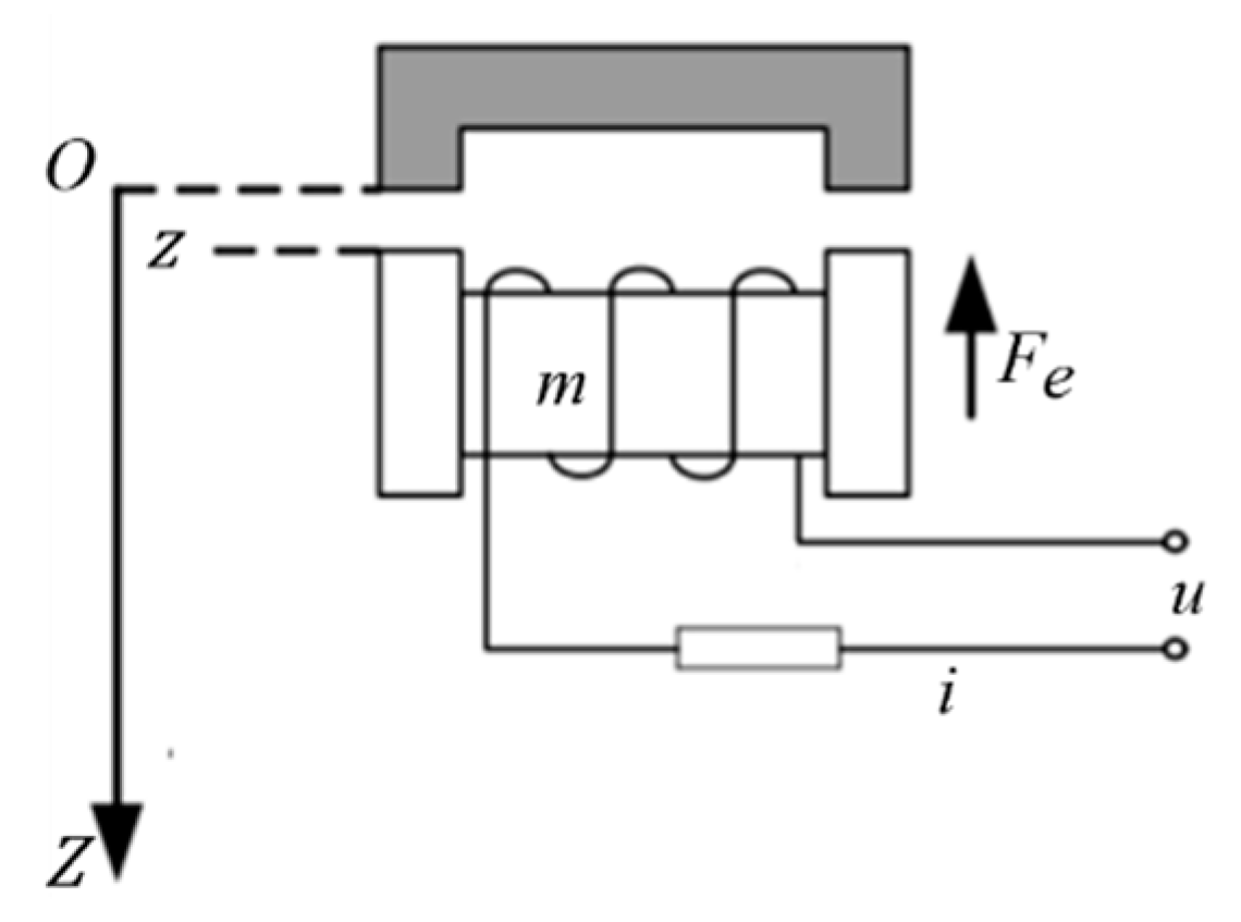
A single-point magnetic levitation system is a technique for levitating an object by electromagnetic force. Its main feature is that a vertical upward electromagnetic force is generated by an electromagnet, which steadily levitates the object in the air. A typical single-point magnetic levitation system is shown in Figure 1, which consists of an electromagnetic coil, an iron core, an armature, and a gap sensor. The electromagnet consists of an electromagnetic coil and an iron core, and the armature is fixed to a bracket. A current is passed through the electromagnetic coil to generate a magnetic field, which passes through the iron core and armature to form a magnetic circuit. The electromagnet generates an upward suction force, and when the suction force is equal to the gravitational force of the electromagnet, the electromagnet will be stably suspended in the air.
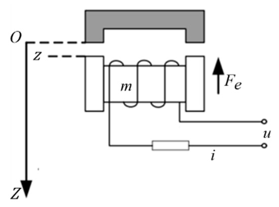
Figure 1.
Single-point magnetic levitation system.
A single-point magnetic levitation system is a typical nonlinear and open-loop unstable system. The magnitude of the electromagnetic force between the electromagnet and the armature is inversely proportional to the distance between them and directly proportional to the current passed in the electromagnetic coil. Just a slight perturbation in the equilibrium state will cause the electromagnet to land or attach itself to the armature and eventually lose its stable suspension. It is therefore necessary to apply closed-loop control to the system in order to keep the electromagnet in a stable levitation state at all times.
The mathematical model of a typical single-point maglev system is shown in Equation (1) [20]:
where m is the mass of the electromagnet; z is the levitation gap of the electromagnet; is the electromagnetic force on the electromagnet; i is the current passed through the electromagnet; u is the voltage at both ends of the electromagnet; is the vacuum permeability; A is the effective magnetic pole conductive area of the electromagnet; n is the number of turns of the electromagnet coil; is the resistance of the electromagnet coil; and K is a constant factor.
The change in gap is a very small quantity compared to the change in current, so the electromagnetic coil can ignore the voltage change caused by the change in gap, and the electromagnetic coil is approximated as a first-order inertial system with an inductor and a resistor in series; therefore, Equation (1) becomes
2.2. Controller Design
Newton’s second law is a macroscopic description of the motion of an object, and it can also describe the motion of a levitated object in a single-point magnetic levitation system. Knowing the electromagnetic force and the mass of the object, the acceleration of the levitated object can be calculated. Therefore, the magnitude of the electromagnetic force directly affects the levitation stability of the levitated object, so the control of the magnitude of the electromagnetic force is a crucial part of whether the magnetic levitation system can levitate stably. For a system in which the material and number of turns of the solenoid coil, the material and volume of the levitated object, and other relevant properties have been determined, the magnitude of the electromagnetic force often depends on the spatial position of the levitated object with respect to the solenoid and the current passed through the solenoid coil. With the relative spatial position determined, the amount of electromagnetic force required depends on the amount of current passing through the electromagnetic coil.
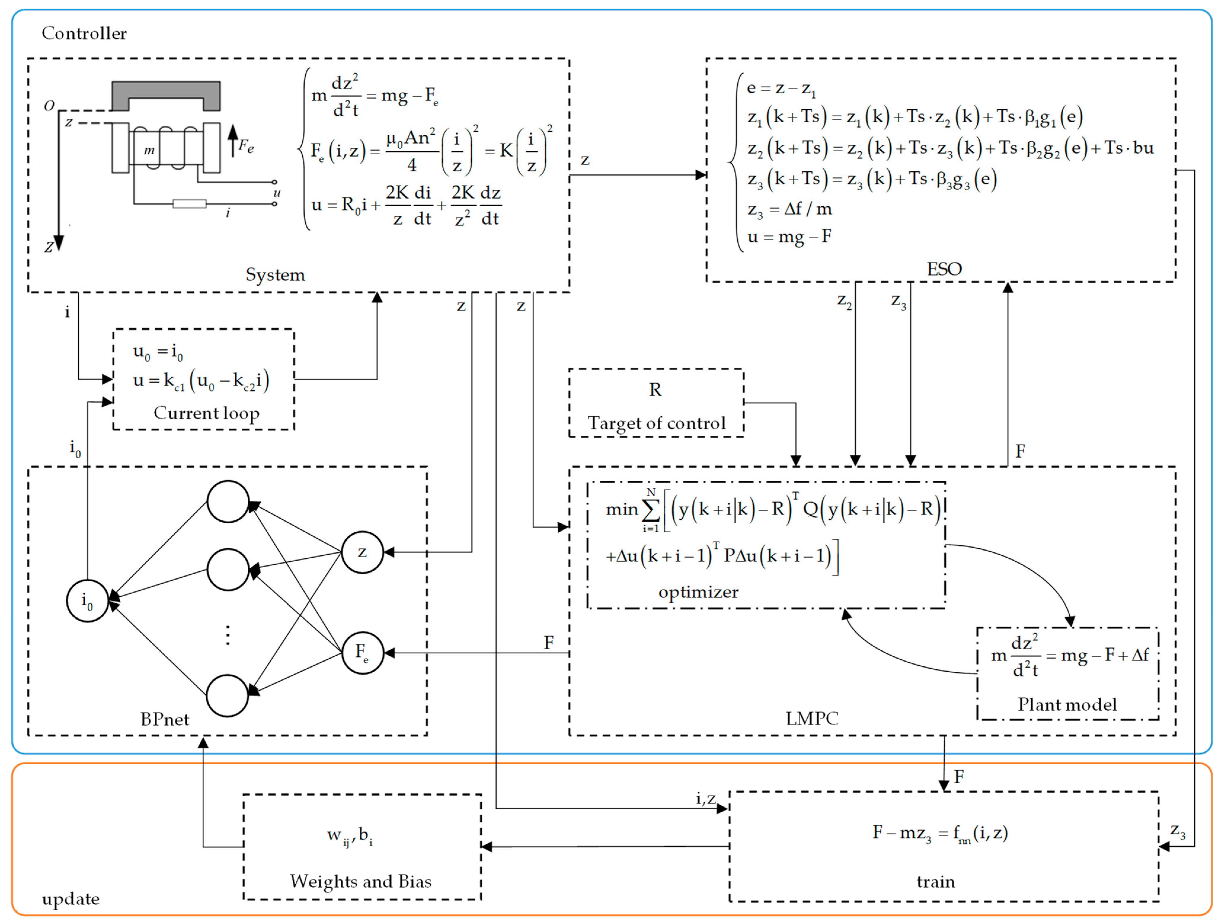
The LMPC-BP controller calculates the required electromagnetic force through the MPC, and then uses a BP neural network to calculate the current required by the electromagnetic coil to generate this electromagnetic force at the current spatial position. Since the electromagnetic coil is a first-order inertial system with inductance and resistance in series, the current signal tracking will be lagged, so the current loop needs to be designed to enhance the tracking speed of the current signal. In addition, the current value required by the electromagnetic force calculated by the BP neural network will have deviation, and the deviation of the current will turn into the deviation of the electromagnetic force which will eventually be shown in the deviation of the acceleration, so that the model motion cannot be levitated in accordance with the planned path, and it may even be destabilized. Therefore, the acceleration deviation due to current deviation needs to be measured by ESO and finally compensated to the MPC controller in the form of electromagnetic force deviation. The charging and discharging of the electromagnet are a typical first-order inertial link, and by designing a suitable current loop, the electromagnet can be treated as a ratio link with a gain of one. Meanwhile, the current signal, position signal combined with the electromagnetic force deviation observed by ESO, and the required electromagnetic force calculated by MPC can be used as new training data to further update the BP neural network. The entire LMPC-BP control block diagram is shown in Figure 2.
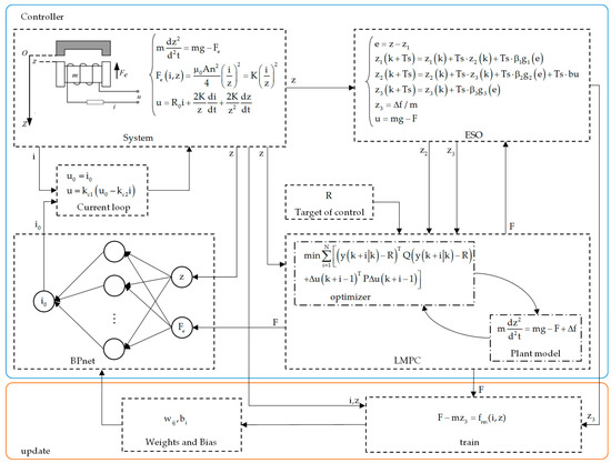
Figure 2.
Structure of the controller.
Each of LPMC, BP neural network prediction model, and ESO will be described in the following.
2.2.1. LMPC
MPC is an advanced control strategy widely used in industrial process control and automation systems. The main idea is to use a model of the system to predict the behavior of the system over a future period of time during each control cycle and to compute a sequence of control inputs that gives the system optimal performance by means of an optimization algorithm. Then, only the first control input in this sequence is used, and the process is repeated after entering the next control cycle.
During the LMPC design process, the electromagnetic force serves as an arbitrarily adjustable input, and how the electromagnetic force is generated is not of concern. Therefore, the prediction model for single-point maglev is reduced to a basic Newton’s second law equation; its prediction model is simplified from Equation (1) to Equation (3):
As a result, the prediction model is reduced to a linear model, which greatly simplifies the computation of the MPC. is the input perturbation. One can take = z and = z, then establish the discrete state space equation in the presence of input perturbations:
where is the state variable of the system; is the control input variable of the system, whose value is the magnitude of the sum of the electromagnetic force and gravity; is the sum of the disturbance; is the state matrix; are the control input matrix and the disturbance input matrix, respectively; is the output matrix; and Ts is the sampling time. The disturbance can be considered as a deviation of the electromagnetic force, so the effect of the disturbance on the system is the same as the effect of the electromagnetic force; so, .
In order to introduce integrals to reduce or eliminate static errors [21], model (4) was rewritten as an incremental model:
where
According to the basic principles of predictive control, the future dynamics of the system are first predicted based on model (5) using the latest measurements as the initial state. For this purpose, the prediction step is set to be N. In order to derive the prediction equations of the system, the following assumptions are made:
- The measurable interference is invariant after moment k, i.e.,
At the current moment (k moments), the measured or observed value is x(k), and is determined. This will be used as an initial value to predict the future dynamics of the system. From model (5), the state increment at the ith moment after k can be predicted as follows:
where denotes the k moment prediction of the state increment at moment k + i, denotes the k moment prediction of the output at moment k + i, and is the k moment prediction of the input increment at moment k + i.
We define the input vector and output vector for N-step prediction as follows:
Then, the output of the future N-step prediction of the system can be calculated using the following prediction Equation (9):
where
For MPC, the cost function is set as follows:
where is a positive-definite diagonal matrix whose parameters on the diagonal correspond to the state’s share in the computation of the cost function. is the target state. It is written in matrix-vector form as follows:
where
Substituting prediction Equation (9) into cost Function (11) reduces it to quadratic programming form by omitting constant terms that are irrelevant to the calculation:
where
Thus, the optimal control sequence at moment k is
The first element of the optimal control sequence is taken to be the actual control input increment to the system:
and the predicted control gain is defined as follows:
Obviously, all parameters in are time-independent constants, so in order to reduce the computational effort, they can be calculated offline by Equation (15). Now, k + 1, the state x(k + 1) and disturbance d(k + 1) are re-measured, the optimal control sequence, now k + 1, is re-computed using the prediction Equation (13), and the first element of the domain system is taken to achieve the rolling optimization.
2.2.2. BP Neural Network Prediction Model
BP neural networks are a multilayer feedforward network trained according to the error back-propagation algorithm and are one of the most widely used neural network models. BP networks are capable of learning and storing a large number of input–output pattern mapping relationships without the need to have the mathematical equations describing such mapping relationships beforehand. Its learning rule is to use the most rapid descent method to continuously adjust the weights and biases of the network by back propagation to minimize the network’s sum of squared errors. The electromagnetic force of an electromagnet is related to the current passed through it and the gap in which it is suspended. For the modeling of the electromagnetic force, this paper builds a network model from the electromagnetic force and gap to the current through a BP neural network, where the electromagnetic force and gap are the inputs, and the current is the output.
where is the mapping relationship between the electromagnetic force and gap to current in the BP neural network.
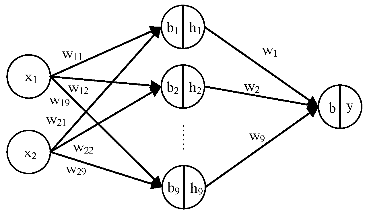
The electromagnetic force solved by LMPC can be used to calculate the current required by the BP neural network. There will be some deviation in the neural network model solving, resulting in the actual electromagnetic force generated by the electromagnet to also deviate from the calculated value. Therefore, it is necessary to introduce the input perturbation when the LMPC theory is derived. And in order to enhance the reduction in computational complexity and improve the computational speed, the number of neurons of the BP neural network is not designed to be large. Its network structure is shown in Figure 3, which is a single hidden layer network structure, and the hidden layer element is 9.
where are the weights of the first and second elements of the output layer to the ith element of the hidden layer and is the bias of the ith element of the hidden layer. is the weight of the ith element of the hidden layer to the output layer and b is the bias of the output layer.

Figure 3.
Network structure.
2.2.3. ESO
To address the problem of bias in network models as well as disturbances, the disturbances need to be observed and compensated by state observers. ESO is a method for state estimation of nonlinear systems. It approximates the unknown system parts by introducing extended state variables and combines them with feedback control to achieve real-time adaptive changes in the system dynamics. ESO has low computational complexity, and at the same time, it can effectively offset modeling errors and measurement noise to improve the accuracy and stability of state estimation. It is widely used in many fields such as machinery control, power systems, the chemical industry, vehicle control, etc. It is an important tool in system monitoring and control.
The state space equations are established based on the single-point maglev dynamics model and the state space is expanded as
where is an expanded state variable that describes the acceleration offset due to disturbances or biases.
Let ; then, the corresponding observer function is
where
are the observer parameters.
2.3. Network Offline Update
It is a very tedious and heavy workload to obtain the data needed for network training through experiments, so it is troublesome to obtain the data through the method of experimental testing. And parametric scanning through finite element software can obtain a large number of relationships between the electromagnetic force, gap, and current, but the data obtained through finite element software are certainly not as good as the experimentally measured data in terms of accuracy, so the electromagnetic force calculated by the trained network will also have a large deviation. As mentioned before, the system can still be stabilized for levitation by feedback deviation through ESO, but when there is a momentary large deviation in the electromagnetic force, ESO often cannot observe accurately in time, so it will affect the system control performance. If the data obtained from finite elements are utilized to train the network, it is necessary to update the network.
The current and position signals are collected. The collected data combined with the electromagnetic force deviation observed by ESO and the required electromagnetic force calculated by MPC can be used as new training data to further update the BP neural network. The flow block diagram is shown in Figure 2, and the added training data are the actual electromagnetic force , the gap z(k), and the current i(k) at time k. Since there is a problem of tracking errors in the values observed by ESO, multiple updates can be implemented to gradually approximate the actual electromagnetic force.
3. Simulation Results and Analysis
A nonlinear electromagnet levitation model was built and simulated to verify the performance of the LMPC-BP controller. The electromagnet related parameters are shown in Table 1.

Table 1.
Electromagnet parameters.
In the table, n is the number of turns of the solenoid coil, R is the resistance of the solenoid, is the vacuum permeability, m is the mass of the solenoid, and A is the effective pole conductive area of the air gap at both ends of the solenoid.
3.1. Step Response
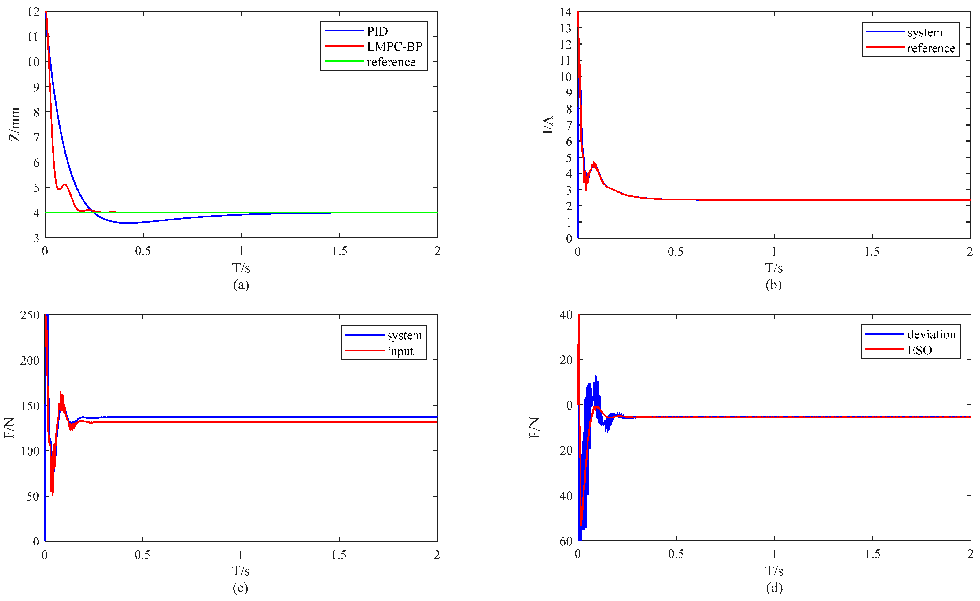
The initial state of this simulation is a 12 mm gap; the target gap is 4 mm, the performance of the LMPC-BP controller and PID controller are compared, and the results are shown in Figure 4 and Table 2. The parameters of PID are selected as Kp = 3000, Ki = 4000, and Kd = 200.
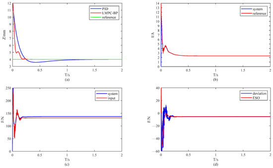
Figure 4.
Step response. (a) Step response; (b) tracking of current signals; (c) deviation between the electromagnetic force calculated by LMPC and the actual electromagnetic force of the system; (d) ESO observations of electromagnetic force deviations.
Table 2.
Step response dynamic performance.
The LMPC-BP controller improves the rise time by 30% and the regulation time by 44.9% with no overshooting compared to the PID controller, as shown in Table 2. Tr, Ts, and σ are the rise time, regulation time, and overshoot of the system. Figure 4b represents the effect of the system current tracking the input reference current, where the system current tracks the reference current at the initial instant and there is no subsequent deviation. Figure 4c represents the deviation between the input to the BP network electromagnetic force and the actual electromagnetic force of the system, and Figure 4d represents the effect of ESO on the observation of the deviation in Figure 4c.
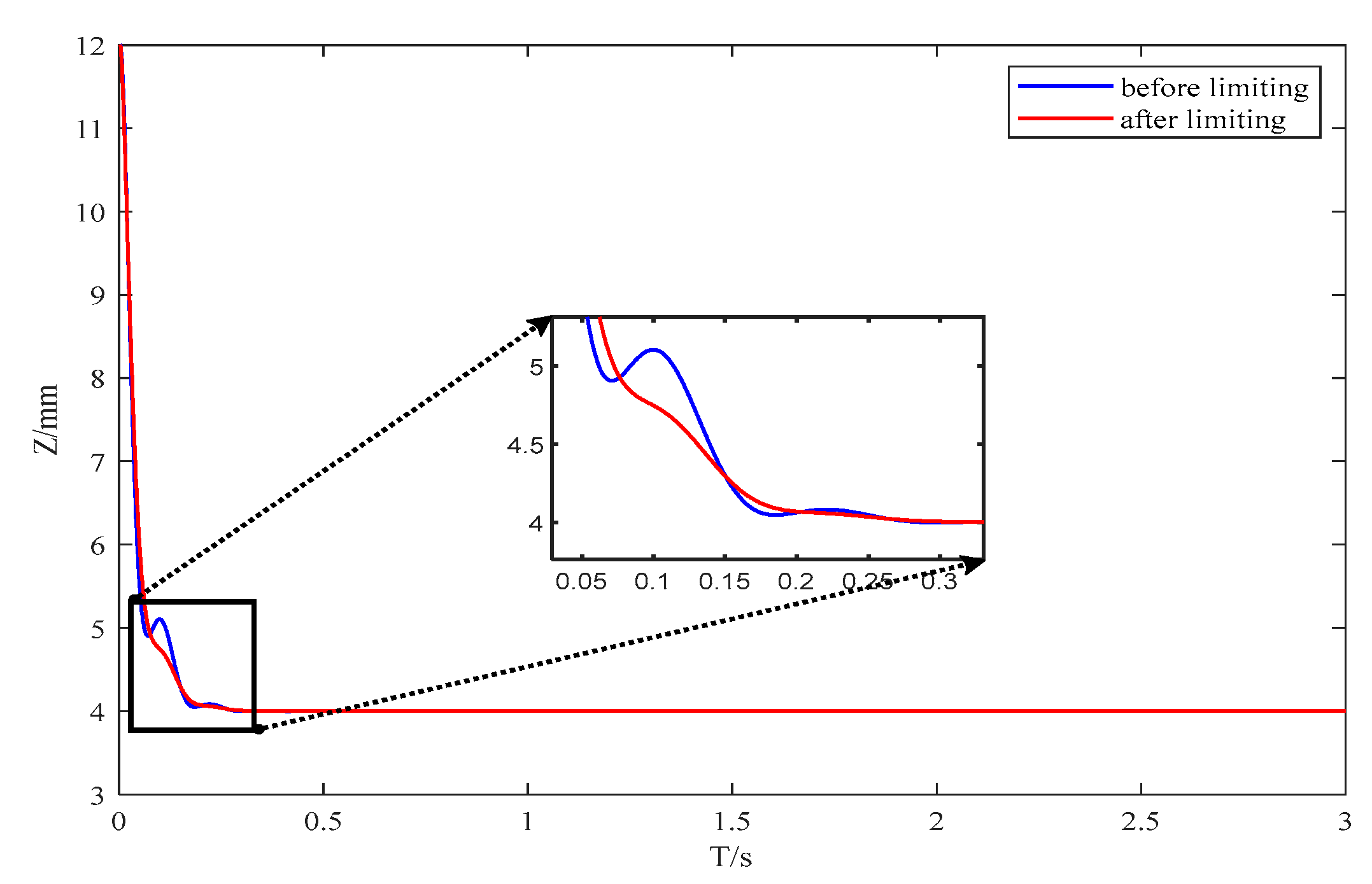
In the initial state, there is a short tracking time for the current, and it is because of this short tracking time that the acceleration of the levitating object is not immediately tracked. Consequently, the ESO observes a large offset, which ultimately causes the LMPC to calculate a large electromagnetic force in order to resist this offset, and after the LMPC adjusts the output in time, the LMPC-BP controller produces a jitter near the initial state. Limiting the amplitude of the output of the ESO can effectively improve this phenomenon, and the results are shown in Figure 5:
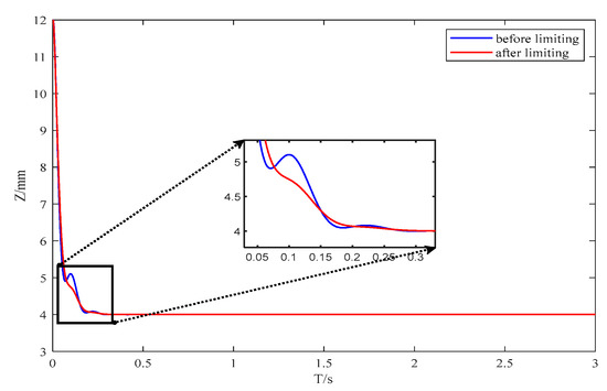
Figure 5.
Performance comparison before and after ESO limiting.
Meanwhile, in practical engineering applications, the slowly rising target signal is used to make the suspension stable, so there will not be a large sudden change in the initial state of the current signal.
3.2. Suspension at Different Gaps
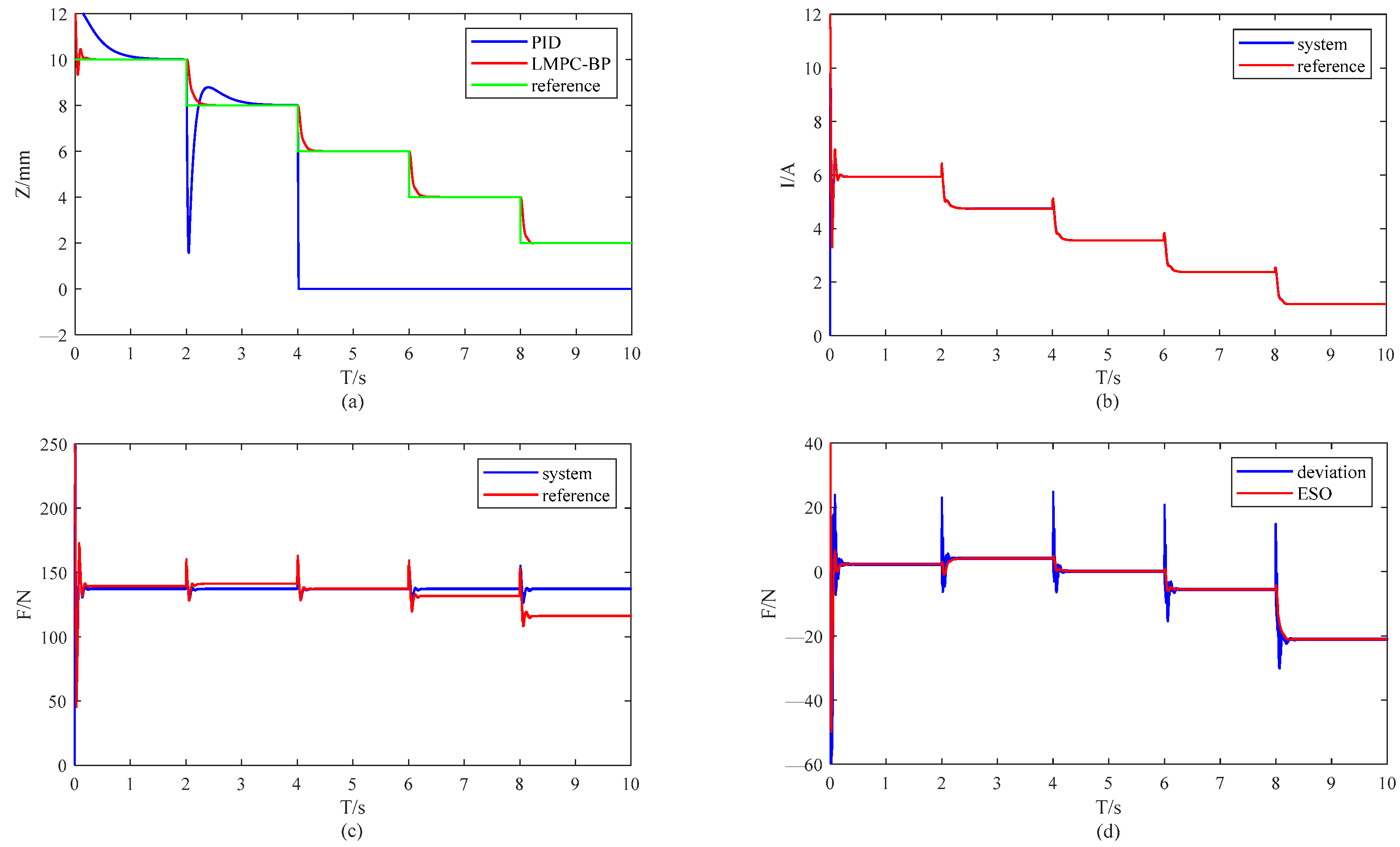
The MSBS needs to suspend the vehicle model in the wind tunnel with different gaps to complete the wind tunnel test, so it needs to complete the variable gap control of the vehicle model using electromagnetic force. That is, after completing the wind tunnel test in the current attitude, the attitude of the model is changed to continue the wind tunnel test. In order to simulate this condition, the target’s levitation gap is changed every two seconds for simulation, and the results are shown in Figure 6.
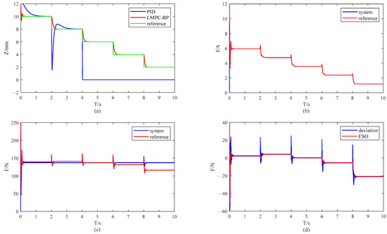
Figure 6.
Variable gap suspension. (a) Variable gap suspension performance comparison; (b) tracking of current signals; (c) deviation between the electromagnetic force calculated by LMPC and the actual electromagnetic force of the system; (d) ESO observations of electromagnetic force deviations.
In the simulation, the LMPC-BP controller stabilized the suspension at different gaps well compared to the PID controller. And except for the first gap change, there was a jitter problem, and since ESO did not see a large “perturbation”, the rest of the gap change operations did not have any jitter.
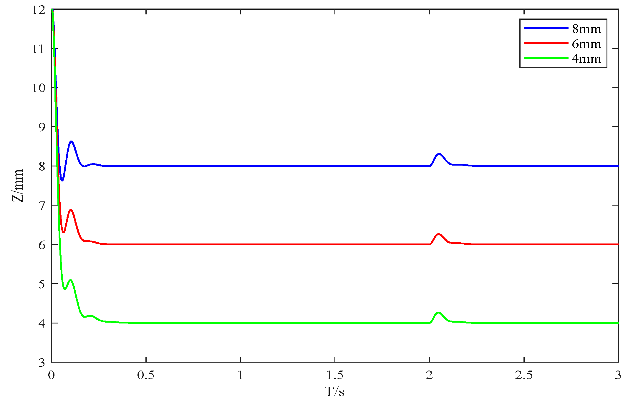
In order to examine the immunity performance of the LMPC-BP controller under different levitation gaps, simulations were carried out under levitation gaps of 4 mm, 6 mm, and 8 mm, respectively. A step interference of 10% of its own gravity was added at 2 s to observe its anti-interference performance. The result is shown in Figure 7.
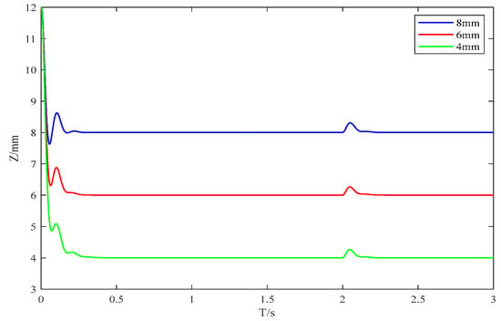
Figure 7.
Antiinterference performance at different gaps.
After applying a step disturbance of 10% of its own gravity, the object stabilized in the three suspension gaps produced a deviation between 0.22 mm and 0.25 mm and returned to a steady state within 0.2 s, so the dynamic performance of the LMPC-BP controller remained almost unchanged with the change in equilibrium.
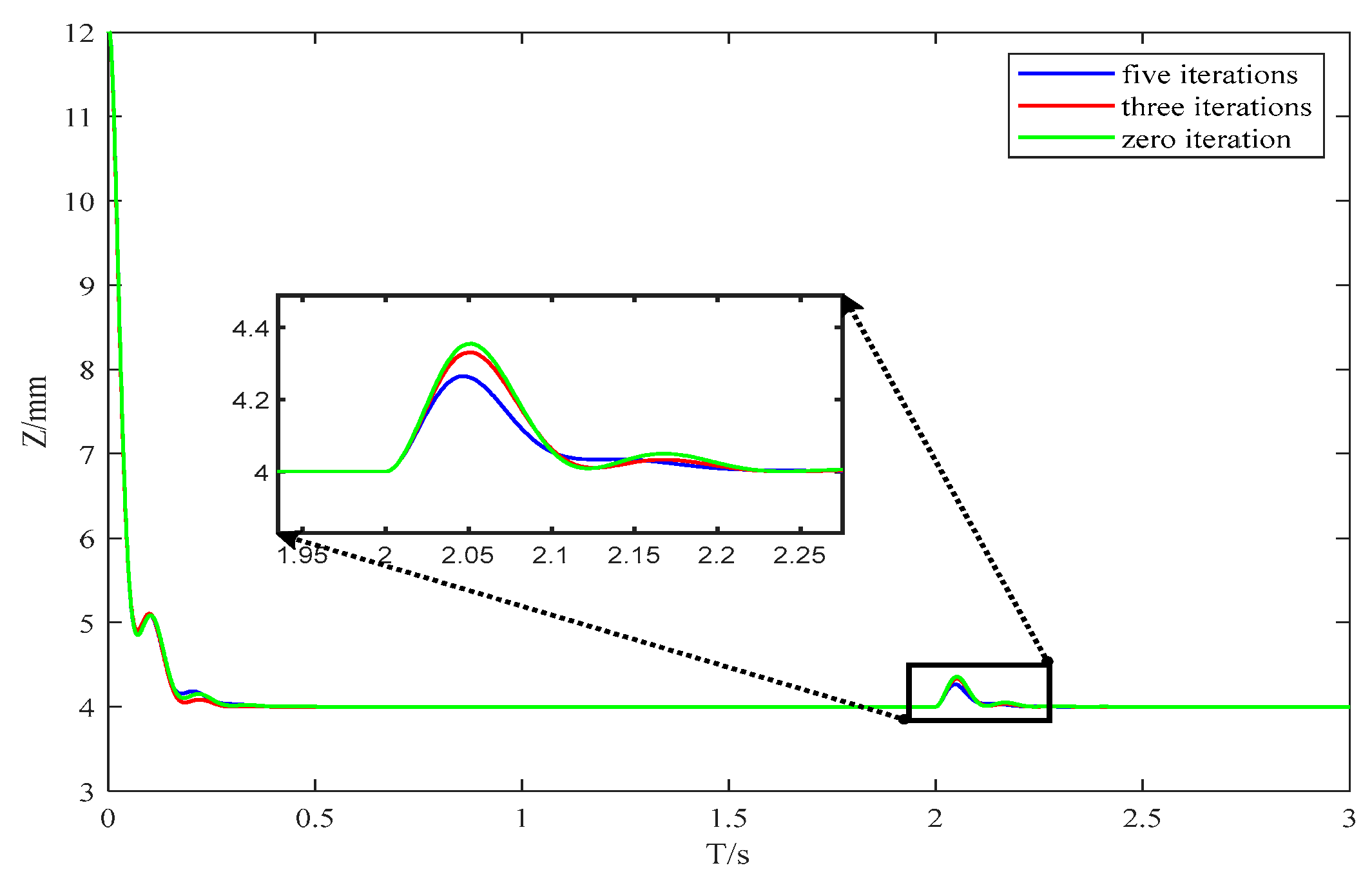
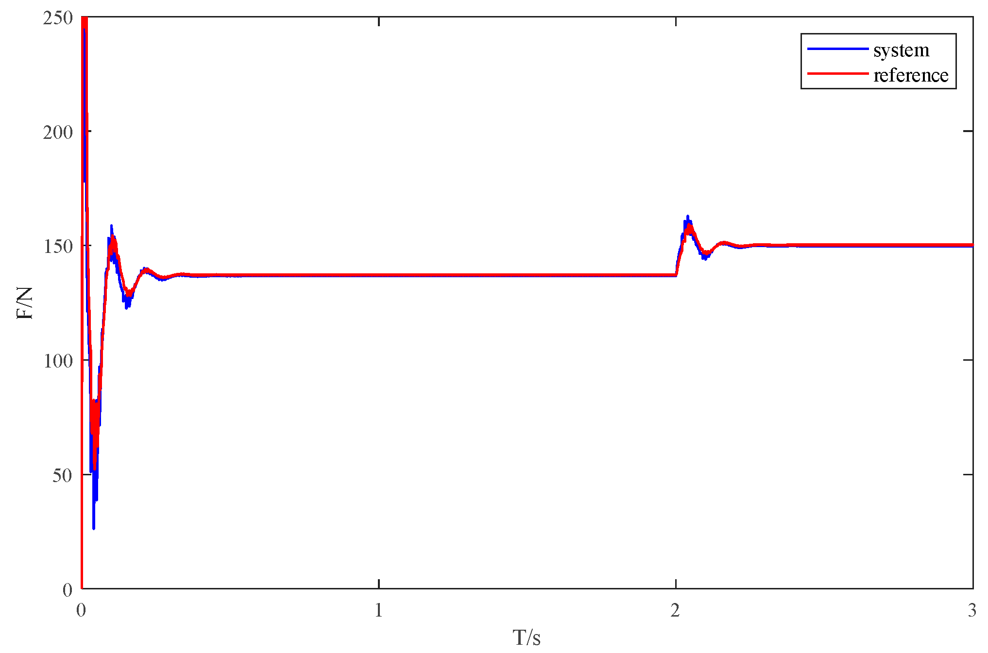
3.3. Comparison of Controller Performance after Updating the Network
In Figure 6c, there is still a large gap between the electromagnetic force calculated by MPC and the electromagnetic force of the system, so it is necessary to correct the coefficients of the BP neural network by updating to make the solution of the current more accurate. After the iteration, the stable suspension as well as the anti-interference performance were tested, and the simulation results are shown in Figure 8.
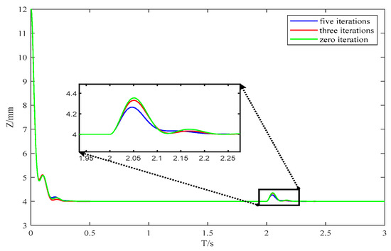
Figure 8.
Anti-disturbance performance of the controller after updating the network.
After the fifth update, the interference resistance of the LMPC-BP controller was improved and there was almost no gap between the calculated electromagnetic force and the electromagnetic force of the system, as shown in Figure 9. Since there was no way to completely eliminate the bias generated by the BP network, the performance was not significantly improved after subsequent network updates.
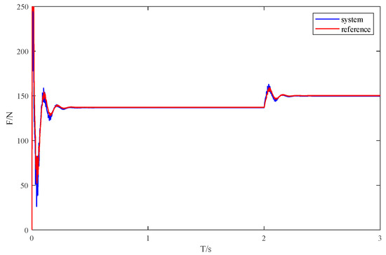
Figure 9.
Deviation between the electromagnetic force calculated by LMPC and the actual electromagnetic force of the system.
4. Conclusions
In this paper, an LMPC-BP controller is designed to improve the dynamic performance compared to traditional PID controllers and to achieve stable levitation of suspended objects with different levitation gaps, where the dynamic performance of the levitation with different gaps does not change significantly. Due to ESO, a BP neural network trained using data from finite element calculations can also stabilize the system for levitation. It is then proposed to re-update the BP neural network using the ESO observation data to improve the anti-disturbance performance of the LMPC-BP controller.
Author Contributions
Conceptualization, Z.L.; methodology, Z.L.; software, Z.L. and F.D.; validation, Z.L. and F.D.; formal analysis, F.D.; investigation, Z.L.; resources, F.D.; data curation, Z.L.; writing—original draft preparation, Z.L.; writing—review and editing, F.D.; visualization, Z.L.; supervision, F.D.; project administration, F.D.; funding acquisition, F.D. All authors have read and agreed to the published version of the manuscript.
Funding
This research was funded by the National Natural Science Foundation of China (Grant No. 52332011).
Data Availability Statement
There is no experimental data in this simulation, and the important conclusions of the simulation are shown in the graphs and tables.
Conflicts of Interest
The authors declare no conflicts of interest.
References
- Yang, F.; Zhao, C.; Bai, Z. A modified electromagnetic force calculation method has high accuracy and applicability for EMS maglev vehicle dynamics simulation. ISA Trans. 2023, 137, 186–198. [Google Scholar] [CrossRef] [PubMed]
- Sun, Y.; Xu, J.; Wu, H. Deep Learning Based Semi-Supervised Control for Vertical Security of Maglev Vehicle With Guaranteed Bounded Airgap. IEEE Trans. Intell. Transp. Syst. 2021, 22, 4431–4442. [Google Scholar] [CrossRef]
- Zhou, T.; Yang, Z.; Zhu, C. Internal model control-PID control of an active magnetic bearing high-speed motor rotor system. Trans. China Electrotech. Soc. 2020, 35, 3414–3425. [Google Scholar]
- Takarli, R.; Amini, A.; Khajueezadeh, M.A. Comprehensive Review on Flywheel Energy Storage Systems: Survey on Electrical Machines, Power Electronics Converters, and Control Systems. IEEE Access 2024, 11, 81224–88125. [Google Scholar] [CrossRef]
- Daiki, K.; Hiroki, S.; Asei, T. Magnetic Suspension and Balance System for High-Subsonic Wind Tunnel. AIAA J. 2019, 57, 2489–2495. [Google Scholar]
- Daiki, K.; Hiroki, S.; Asei, T. Dynamic Wind-Tunnel Testing of a Sixty-Degree Delta-Wing Model Without Support Interference. AIAA J. 2021, 59, 1099–1108. [Google Scholar]
- Liu, L.; Zuo, J. Parameter self-adjusting control method of fuzzy PID for magnetic levitation ball system. J. Control Eng. 2021, 28, 354–359. [Google Scholar]
- Marcin, M.; Arkadiusz, L. Speed observer structure of induction machine based on sliding super-twisting and backstepping techniques. IEEE Trans. Ind. Inform. 2021, 17, 1122–1131. [Google Scholar]
- Zhang, T.; Xu, Z.; Li, J. A third-order super-twisting extended state observer for dynamic performance enhancement of sensorless IPMSM drives. IEEE Trans. Ind. Electron. 2021, 67, 5948–5958. [Google Scholar] [CrossRef]
- He, L. Auto-Disturbance-Rejection Control of Maglev System; National University of Defense Technology: Changsha, China, 2006. [Google Scholar]
- Wei, Q.; Wu, Z.; Zhou, Y. Active Disturbance-Rejection Controller (ADRC)-Based Torque Control for a Pneumatic Rotary Actuator with Positional Interference. Actuators 2024, 13, 66. [Google Scholar] [CrossRef]
- Chen, C.; Sun, Y. Research on dynamics modeling and control of the nonlinear maglev system. Mach. Des. Manuf. 2019, 11, 16–19. [Google Scholar]
- Sun, Y.; Qiang, H.; Wan, L. A Fuzzy-Logic-System-Based Cooperative Control for the Multielectromagnets Suspension System of Maglev Trains With Experimental Verification. IEEE Trans. Fuzzy Syst. 2023, 31, 3411–3422. [Google Scholar] [CrossRef]
- Tao, L.; Wang, P.; Ma, X. Variable Form LADRC-Based Robustness Improvement for Electrical Load Interface in Microgrid: A Disturbance Response Perspective. IEEE Trans. Ind. Inform. 2024, 20, 432–441. [Google Scholar] [CrossRef]
- Ren, Y.M.; Alhajeri, M.S.; Luo, J.; Chen, S.; Abdullah, F.; Wu, Z.; Christofides, P.D. A tutorial review of neural network modeling approaches for model predictive control. Comput. Chem. Eng. 2022, 165, 107956. [Google Scholar] [CrossRef]
- Xiao, L.; Xu, M.; Chen, Y. Hybrid Grey Wolf Optimization Nonlinear Model Predictive Control for Aircraft Engines Based on an Elastic BP Neural Network. Appl. Sci. 2019, 9, 1254. [Google Scholar] [CrossRef]
- Grady, W.; Nolan, W.; Brian, G. Information theoretic MPC for model-based reinforcement learning. In Proceedings of the IEEE International Conference on Robotics and Automation, Singapore, 29 May–3 June 2017; pp. 1714–1721. [Google Scholar]
- Nagabandi, A.; Kahn, G.; Fearing, R.S. Neural Network Dynamics for Model-Based Deep Reinforcement Learning with Model-Free Fine-Tuning. In Proceedings of the IEEE International Conference on Robotics and Automation, Brisbane, QLD, Australia, 21–25 May 2018; pp. 7559–7566. [Google Scholar]
- Iman, A.; Babak, B.; Thomas, W. Sampling-Based Nonlinear MPC of Neural Network Dynamics with Application to Autonomous Vehicle Motion Planning. In Proceedings of the 2022 American Control Conference, Atlanta, GA, USA, 8–10 June 2022; pp. 2084–2090. [Google Scholar]
- Sun, Y.; Xu, J.; Chen, C. Reinforcement learning-based optimal tracking control for levitation system of maglev vehicle with input time delay. IEEE Trans. Instrum. Meas. 2022, 71, 1–13. [Google Scholar] [CrossRef]
- Giulio, B.; Marcello, F.; Riccardo, S. A robust MPC algorithm for offset-Free tracking of constant reference signals. IEEE Trans. Autom. Control 2013, 58, 2394–2400. [Google Scholar]
Disclaimer/Publisher’s Note: The statements, opinions and data contained in all publications are solely those of the individual author(s) and contributor(s) and not of MDPI and/or the editor(s). MDPI and/or the editor(s) disclaim responsibility for any injury to people or property resulting from any ideas, methods, instructions or products referred to in the content. |
© 2024 by the authors. Licensee MDPI, Basel, Switzerland. This article is an open access article distributed under the terms and conditions of the Creative Commons Attribution (CC BY) license (https://creativecommons.org/licenses/by/4.0/).