Article

Stiffness Analysis of Cable-Driven Parallel Robot for UAV Aerial Recovery System

1
School of Mechatronics Engineering, Harbin Institute of Technology, Harbin 150001, China
2
State Key Laboratory of Robotics and System, Harbin Institute of Technology, Harbin 150001, China
*
Authors to whom correspondence should be addressed.
Actuators 2024, 13(9), 343; https://doi.org/10.3390/act13090343
Submission received: 19 July 2024 / Revised: 4 September 2024 / Accepted: 5 September 2024 / Published: 6 September 2024
(This article belongs to the Special Issue Soft Robotics: Actuation, Control, and Application)

Abstract

:
Unmanned Aerial Vehicle (UAV) aerial recovery is a challenging task due to the limited maneuverability of both the transport aircraft and the UAV, making it difficult to establish an effective capture connection in the airflow field. In previous studies, we proposed using a Cable-Driven Parallel Robot (CDPR) for active interception and recovery of UAVs. However, during the aerial recovery process, the CDPR is continuously subjected to aerodynamic loads, which significantly affect the stiffness characteristics of the CDPR. This paper conducts a stiffness analysis of a single cable and a CDPR in a flow field environment. Firstly, we derive the stiffness matrix of a single cable based on a model that considers aerodynamic loads. The CDPR is then divided into elements using the finite element method (FEM), and the stiffness matrix for each element is obtained. These element stiffness matrices are assembled to form the stiffness matrix of the CDPR system. Secondly, we analyze the stiffness distribution of a single cable at various equilibrium positions within a flow field environment. Aerodynamic loads were observed to alter the equilibrium position of the cable, thereby impacting its stiffness. The more the cable bends, the greater the reduction in its stiffness. We examine the stiffness distribution characteristics of the CDPR’s end-effector within its workspace and analyze the impact of varying flow velocities and different cable materials on the system’s stiffness. This research offers a methodology for analyzing the stiffness of CDPR systems operating in a flow field environment.

1. Introduction

In recent years, UAV technology has rapidly advanced, playing an increasingly important role in various applications. UAV aerial recovery involves retrieving and reusing UAVs in mid-air using transport aircraft [1]. This technology offers several advantages, such as expanding operational ranges, enabling rapid reloading and reuse, enhancing flexibility, and reducing reliance on land-based or sea-based landing infrastructure [2,3,4]. However, the limited maneuverability of transport aircraft and UAVs, combined with the challenges of performing recovery operations in mid-air, makes this task extremely difficult. To date, only a few successful UAV aerial recovery operations have been documented [5]. This project uses a flexible towed cable–drogue scheme, but this configuration suffers from low stiffness due to its flexible cable, making it susceptible to gusts and aerodynamic coupling forces during docking. These factors significantly increase the challenge of achieving successful recovery.
However, another potential UAV aerial recovery system is the CDPR. In previous research [6], we proposed a CDPR structure combining a rigid telescopic rod with four suspension cables (as shown in Figure 1). The telescopic rod provides more precise directional control and support for the suspension cables. By adjusting the lengths of the cables and the telescopic rod, we can control the position of the CDPR’s end-effector. This CDPR has the advantage of reducing the control requirements on the UAV itself, offering greater stiffness for the recovery platform, and better adapting to complex flow field environments, making the recovery operation more versatile.
CDPRs are widely used in various fields due to their simple structure, large workspace, and high load capacity [7,8]. Stiffness is one of the most important performance indicators of robots. It is essential to study the stiffness of cable-driven parallel robots, as this has significant implications for system stability analysis, dynamic response analysis, and overall control strategies. In the context of CDPRs, stiffness is commonly defined as the ratio of the infinitesimal change in the force exerted on the end-effector to the resulting infinitesimal displacement. Elastic cables are often modeled using a spring analogy, leading to stiffness matrices that include geometric stiffness and cable stiffness components. The geometric stiffness matrix depends on the CDPR’s configuration and cable tensions, with its key calculation involving the Hessian matrix. Meanwhile, the cable stiffness matrix varies with the CDPR’s configuration, pose, and material properties [9]. In redundant CDPRs, adjusting the magnitude of cable tensions allows for tuning the system’s stiffness. Kawamura et al. [10] conducted a stiffness analysis study on the parallel cable-driven high-speed robot FALCON-7. Their findings indicated that increasing cable tensions can improve structural stiffness. Cui et al. [11,12] studied the impact of the structural design on the stiffness and controllability of CDPRs. Gueners et al. [13] proposed an anchor point optimization method for maximizing rigidity in 3D-printed CDPRs, analyzing how pre-tensioning within cables affects platform stiffness. In large-span CDPR structures, the mass of cables cannot be ignored. The “sagging cable” model [14,15] is used in CDPRs. Yuan et al. [16] analyzed the static and dynamic stiffness of CDPRs, considering the effect of both cable mass and elasticity. They evaluated the static stiffness by the variation of the end-effector pose error and analyzed the dynamic stiffness by identifying the robot’s natural frequencies. Arsenault [17] studied the effect of cable sag in a spatial parallel three-degree-of-freedom suspended cable-driven mechanism on workspace and stiffness. Most previous papers analyzed the stiffness of CDPRs in non-flow environments. However, in flow environments, CDPRs are subjected to aerodynamic forces. Specifically, flexible cables bend under these aerodynamic forces, which consequently impacts the system’s stiffness. However, there are few papers in which the CDPRs are used in a flow field environment. Gao et al. [18] studied a flying CDPR with eight cables, analyzing the overall analytical expression of the stiffness matrix. However, their analysis did not consider the impact of aerodynamic loads on the CDPR during flight. Studying the stiffness distribution characteristics and influencing factors of CDPRs enables overall stiffness adjustments, enhancing the robot’s flexibility and controllability. In this paper, based on the cable model considering aerodynamic loads, we derive the stiffness matrix for a single cable. Our analysis shows that aerodynamic loads significantly impact the stiffness of the cable, and this effect is related to the angle between the cable and the flow direction. Using the stiffness of both cable and rod elements, we assemble the stiffness matrix for the CDPR system. We then analyze the stiffness distribution characteristics of the CDPR system within its reachable workspace and investigate the effects of different flow velocities and cable materials on system stiffness. Additionally, we derive a simplified expression for the end-effector stiffness matrix of the CDPR when the cable stiffness is much lower than the rod stiffness.
The content of this paper is organized as follows: Section 2 introduces the single cable model, taking into account aerodynamic loads, and derives the single cable stiffness matrix. Section 3 explains the use of the finite element method (FEM) to decompose the system structure into elements, determine the stiffness of each element, and assemble the overall system stiffness of the CDPR. Section 4 analyzes both the single cable stiffness and the CDPR system stiffness, including the distribution of stiffness and the factors that affect it. Section 5 summarizes the research findings on CDPR stiffness.

2. Stiffness of the Cable Considering Aerodynamic Loads

It was assumed that one end of the cable is fixed at point A , and the tension at the other end, point B , is represented by the components ( t B x , t B y , t B z ) . The static equilibrium forces of the cable in the airflow field are shown in Figure 2.
In a previous study [6], we developed a spatial cable model that considers the elasticity, mass, and aerodynamic loads of the cable simultaneously. Notably, the model assumes the cable is taut and has minimal spatial bending. Let l = L 0 , the analytical expression for the coordinates of the endpoint B of the cable is then obtained as follows.
B x = t Bx L 0 EA + k x L 0 2 2 EA + k x ( b 4 b 1 ) b 3 + ( t Bx b 3 b 2 k x 2 b 3 3 / 2 ) ln ( 0 . 5 b 2 + b 3 L 0 + b 4 b 3 0 . 5 b 2 + b 1 b 3 ) B y = t By L 0 EA + k y L 0 2 2 EA + k y ( b 4 b 1 ) b 3 + ( t By b 3 b 2 k y 2 b 3 3 / 2 ) ln ( 0 . 5 b 2 + b 3 L 0 + b 4 b 3 0 . 5 b 2 + b 1 b 3 ) B z = t Bz L 0 EA + ( k z + ρ c Ag ) L 0 2 2 EA + ( k z + ρ c Ag ) ( b 4 b 1 ) b 3 + ( t Bz b 3 b 2 ( k z + ρ c Ag ) 2 b 3 3 / 2 ) ln ( 0 . 5 b 2 + b 3 L 0 + b 4 b 3 0 . 5 b 2 + b 1 b 3 )
where k x = 1 2 ρ a D c n v x a 2 t Bx a 1 a 2 3 / 2 a 3 a 2 a 1 2 + 1 2 ρ a π D c t t Bx a 1 a 1 a 2 3 / 2 , k y = 1 2 ρ a D c n v y a 2 t By a 1 a 2 3 / 2 a 3 a 2 a 1 2 + 1 2 ρ a π D c t t By a 1 a 1 a 2 3 / 2 , k z = 1 2 ρ a D c n v z a 2 t Bz a 1 a 2 3 / 2 a 3 a 2 a 1 2 + 1 2 ρ a π D c t t Bz a 1 a 1 a 2 3 / 2 , a 1 = t Bx v x + t By v y + t Bz v z , a 3 = v x 2 + v y 2 + v z 2 , a 2 = b 1 = t Bx 2 + t By 2 + t Bz 2 , b 1 = t Bx 2 + t By 2 + t Bz 2 , b 2 = 2 t By k y + 2 t Bx k x + 2 t Bz ( k z + ρ c Ag ) , b 3 = k x 2 + k y 2 + ( k z + ρ c Ag ) 2 , b 4 = b 1 + b 2 L 0 + b 3 L 0 2 .
The parameter symbols in Equation (1) correspond to the parameter names provided in Table 1.
From Equation (1), it can be seen that B x , B y , and B z are functions of t Bx , t By , and t Bz .
B x = f x ( t Bx , t By , t Bz ) B y = f y ( t Bx , t By , t Bz ) B z = f z ( t Bx , t By , t Bz )
The flexibility matrix C l of the cable is represented as follows:
C l = f x t Bx f x t By f x t Bz f y t Bx f y t By f y t Bz f z t Bx f z t By f z t Bz
Based on the flexibility matrix C l , the cable stiffness matrix K l can be determined.
K l = C l 1 = k 11 k 12 k 13 k 21 k 22 k 23 k 31 k 32 k 33

3. Stiffness Calculation of the CDPR

Figure 3 shows the structure layout of the UAV aerial recovery system. In the Figure, A x y z denotes the body coordinate system of the carrier, with the x -axis pointing in the direction of flight. On the same plane, point A is the endpoint of the telescopic rod, while A 1 , A 2 , A 3 , and A 4 are the suspension points of the four cables.

3.1. Global Coordinates and Elements Stiffness of CDPR

In the UAV recovery system, the CDPR is composed of cables and a telescopic rod, and its stiffness can be calculated using the direct stiffness method [19]. In Figure 4, a global coordinate system A X Y Z is established, where its origin coincides with the origin of the body coordinate system A x y z . The X direction points towards the endpoint P , the Y direction is perpendicular to line A P , and always lies in the plane with x -axes (the body coordinate system of the carrier) and A P . The CDPR is divided into elements, and nodes are defined, with elements numbered using square numbers and nodes numbered using circle numbers. The degrees of freedom for each node are defined with red numbers, as shown in Figure 4. To facilitate the calculation of the system stiffness, the system is divided into three parts: the four parallel cables, the telescopic rod, and the extension rod. The stiffness of each part is calculated separately and then assembled into the overall system stiffness.
The stiffness matrix of the cable element in the body coordinate system is represented as K l i ( i = 1 , 2 , 3 , 4 ) , which has been derived in previous sections and is a 3 × 3 matrix. Consequently, it is straightforward to obtain the overall stiffness matrix for the four-parallel-cables system formed by elements 1, 2, 3, and 4 as follows:
K c = T T ( i = 1 4 K l i ) T = k 11 c k 12 c k 13 c k 21 c k 22 c k 23 c k 31 c k 32 c k 33 c
where T is the element transformation matrix. Expressed using the coordinates of point B ( B x , B y , B z ) as follows:
T = B x B x 2 + B y 2 + B z 2 0 B y 2 + B z 2 B x 2 + B y 2 + B z 2 B z B x 2 + B y 2 + B z 2 B y B y 2 + B z 2 B x B z ( B y 2 + B z 2 ) ( B x 2 + B y 2 + B z 2 ) B y B x 2 + B y 2 + B z 2 B z B y 2 + B z 2 B x B y ( B y 2 + B z 2 ) ( B x 2 + B y 2 + B z 2 )
In Figure 5, for the telescopic rod (element 5), the local coordinate system is aligned with the global coordinate system, and the degrees of freedom for each node are defined with red numbers. To obtain the stiffness matrix of element 5, we first consider it as consisting of three short rods, with material properties including Young’s modulus E and shear modulus G . The length, cross-sectional area, moments of inertia about the two principal axes, and polar moment of inertia for the i th short rod are denoted as L i , A i , I 1 i , I 2 i , J i ( i = 1 , 2 , 3 ) respectively. The relationship between lengths satisfies the equation L 2 = L 3 = ( A B L 1 ) / 2 . The general form [19] of the stiffness matrix for each short rod in the local coordinate system of the 12-degree-of-freedom frame element is as follows.
K = E I l 3 A l 2 I 0 0 0 0 0 A l 2 I 0 0 0 0 0 0 12 0 0 0 6 l 0 12 0 0 0 6 l 0 0 12 0 6 l 0 0 0 12 0 6 l 0 0 0 0 G J l 2 E I 0 0 0 0 0 G J l 2 E I 0 0 0 0 6 l 0 4 l 2 0 0 0 6 l 0 2 l 2 0 0 6 l 0 0 0 4 l 2 0 6 l 0 0 0 2 l 2 A l 2 I 0 0 0 0 0 A l 2 I 0 0 0 0 0 0 12 0 0 0 6 l 0 12 0 0 0 6 l 0 0 12 0 6 l 0 0 0 12 0 6 l 0 0 0 0 G J l 2 E I 0 0 0 0 0 G J l 2 E I 0 0 0 0 6 l 0 2 l 2 0 0 0 6 l 0 4 l 2 0 0 6 l 0 0 0 2 l 2 0 6 l 0 0 0 4 l 2
Through FEM assembly, a 24 × 24 stiffness matrix can be obtained. However, in the CDPR system studied in this paper, the telescopic rod between multiple sections features cylindrical fits, and the bending stiffness of the telescopic rods is provided by the outer sleeves. In fact, aerodynamic loads and gravitational force have minimal effects on the deformation of high-stiffness telescopic rods. When calculating the stiffness of each element, we neglect the effects of small deformations. Simultaneously, we exclude released degrees of freedom 5 and 6, as well as degrees of freedom 1, 2, 3, and 4, whose displacements are constrained. This yields the stiffness matrix of element 5 in the global coordinate system, where the rows and columns correspond to global coordinates as follows: 13, 14, 15, 16, 17, 18, 1, 2, 3, 4, 5, 6.
K 5 = a 1 0 0 0 0 0 a 1 0 0 0 0 0 0 a 4 0 0 0 0 0 a 4 0 0 0 a 3 0 0 a 4 0 0 0 0 0 a 4 0 a 3 0 0 0 0 G J 1 l 1 0 0 0 0 0 G J 1 l 1 0 0 0 0 a 5 0 a 2 0 0 0 a 5 0 a 6 0 0 a 5 0 0 0 a 2 0 a 5 0 0 0 a 6 a 1 0 0 0 0 0 a 1 0 0 0 0 0 0 a 4 0 0 0 0 0 a 4 0 0 0 a 3 0 0 a 4 0 0 0 0 0 a 4 0 a 3 0 0 0 0 G J 1 l 1 0 0 0 0 0 G J 1 l 1 0 0 0 0 a 3 0 0 0 0 0 a 3 0 a 7 0 0 a 3 0 0 0 0 0 a 3 0 0 0 a 7
where a 1 = E A 1 A 2 A 3 A 1 A 2 l 2 + A 1 A 3 l 2 + A 2 A 3 l 1 , a 2 = 4 E I 1 l 1 , a 3 = 3 E I 1 I 2 I 3 ( l 1 + 2 l 2 ) a 8 , a 4 = 3 E I 1 I 2 I 3 a 8 , a 5 = 6 E I 1 ( 3 I 1 I 2 l 2 2 + I 1 I 3 l 2 2 + I 2 I 3 l 1 2 + 2 I 1 I 2 l 1 l 2 + 2 I 1 I 3 l 1 l 2 ) l 1 a 8 , a 6 = 2 E I 1 ( 4 I 1 I 2 l 2 3 + 4 I 1 I 3 l 2 3 + I 2 I 3 l 1 3 + 3 I 1 I 2 l 1 l 2 2 + 9 I 1 I 3 l 1 l 2 2 + 6 I 2 I 3 l 1 2 l 2 ) l 1 a 8 , a 7 = 3 E I 1 I 2 I 3 ( l 1 + 2 l 2 ) 2 a 8 , a 8 = 7 I 1 I 2 l 2 3 + I 1 I 3 l 2 3 + I 2 I 3 l 1 3 + 9 I 1 I 2 l 1 l 2 2 + 3 I 1 I 2 l 1 2 l 2 + 3 I 1 I 3 l 1 l 2 2 + 3 I 1 I 3 l 1 2 l 2 .

3.2. CDPR Stiffness Matrix

Element 6 is a standard 12-degree-of-freedom frame element. Therefore, by assembling the stiffness matrices of each element, we obtain the 18 × 18 CDPR stiffness matrix K c d p r , with the rows and columns corresponding to coordinates 1 through 18.
K c d p r = a 1 + E A 3 l 4 + k 11 c k 12 c k 13 c 0 0 0 E A 3 l 4 0 0 0 0 0 a 1 0 0 0 0 0 k 12 c a 4 + 12 E I 3 l 4 3 + k 22 c k 23 c 0 0 6 E I 3 l 4 2 a 3 0 12 E I 3 l 4 3 0 0 0 6 E I 3 l 4 2 0 a 4 0 0 0 0 k 31 c k 32 c a 4 + 12 E I 3 l 4 3 + k 33 c 0 a 3 6 E I 3 l 4 2 0 0 0 12 E I 3 l 4 3 0 6 E I 3 l 4 2 0 0 0 a 4 0 0 0 0 0 0 G J 1 l 1 + G J 3 l 4 0 0 0 0 0 G J 3 l 4 0 0 0 0 0 G J 1 l 1 0 0 0 0 a 3 6 E I 3 l 4 2 0 a 7 + 4 E I 3 l 4 0 0 0 6 E I 3 l 4 2 0 2 E I 3 l 4 0 0 0 a 3 0 0 0 0 6 E I 3 l 4 2 a 3 0 0 0 a 7 + 4 E I 3 l 4 0 6 E I 3 l 4 2 0 0 0 2 E I 3 l 4 0 a 3 0 0 0 0 E A 3 l 4 0 0 0 0 0 E A 3 l 4 0 0 0 0 0 0 0 0 0 0 0 0 12 E I 3 l 4 3 0 0 0 6 E I 3 l 4 2 0 12 E I 3 l 4 3 0 0 0 6 E I 3 l 4 2 0 0 0 0 0 0 0 0 12 E I 3 l 4 3 0 6 E I 3 l 4 2 0 0 0 12 E I 3 l 4 3 0 6 E I 3 l 4 2 0 0 0 0 0 0 0 0 0 0 G J 3 l 4 0 0 0 0 0 G J 3 l 4 0 0 0 0 0 0 0 0 0 0 6 E I 3 l 4 2 0 2 E I 3 l 4 0 0 0 6 E I 3 l 4 2 0 4 E I 3 l 4 0 0 0 0 0 0 0 0 6 E I 3 l 4 2 0 0 0 2 E I 3 l 4 0 6 E I 3 l 4 2 0 0 0 4 E I 3 l 4 0 0 0 0 0 0 a 1 0 0 0 0 0 0 0 0 0 0 0 a 1 0 0 0 0 0 0 a 4 0 0 0 0 0 0 0 0 0 0 0 a 4 0 0 0 a 6 0 0 a 4 0 0 0 0 0 0 0 0 0 0 0 a 4 0 a 6 0 0 0 0 G J 1 l 1 0 0 0 0 0 0 0 0 0 0 0 G J 1 l 1 0 0 0 0 a 3 0 0 0 0 0 0 0 0 0 0 0 a 5 0 a 2 0 0 a 3 0 0 0 0 0 0 0 0 0 0 0 a 5 0 0 0 a 2
However, we are more concerned with the stiffness of the robot end-effector when the CDPR is in equilibrium within a flow field environment. Assuming the change in external load at point B is zero, we can derive a 3 × 3 stiffness matrix K P for the robot end-effector from the K c d p r matrix. This is achieved by removing the constrained degrees of freedom 13, 14, and 15 and eliminating the released degrees of freedom 1, 2, 3, 4, 5, 6, 10, 11, 12, 16, 17, 18. Throughout the remainder of this paper, the term “CDPR stiffness” will refer to the end-effector stiffness K P .

4. Stiffness Analysis

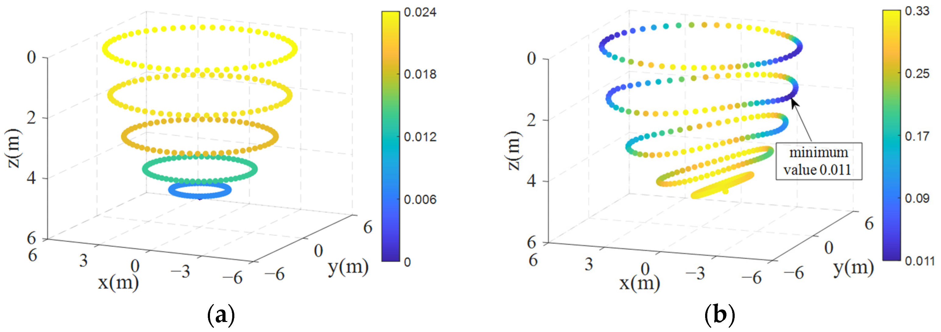
4.1. Analysis of Single Cable Stiffness in Flow Field Environment

In reference [20], the effect of sagging caused by self-mass on the stiffness of cables was studied. However, the UAV aerial recovery system examined in this paper operates in an airflow field, where aerodynamic loads, along with the UAV’s own weight, cause the cables to bend. This bending alters the stiffness of the cables. The following analysis focuses on the stiffness of the cables in this flow field environment.
We analyze the spatial equilibrium position of a single cable under different conditions and provide a set of analysis parameters: at an altitude of 3 km, with an atmospheric density ρ w = 0.9096   kg / m 3 . One end of a cable, considering its mass and elasticity, is fixed at point A , while the other end at point B has a tension of 100 N . The cable length L 0 = 5   m , diameter d s = 0 . 0 2   m , and cable density ρ c = 0.0785   kg / m , the elastic modulus E = 1.6   GPa , the flow field velocity is 40   m / s , and the aerodynamic parameters are C t = 0.02 , C n = 0.8 .
When considering only the length and tension of the cables, the set of equilibrium points in space forms a hemispherical surface (limited to the + z -axis side). Under different influencing factors, these surfaces vary. However, it is challenging to observe how these factors affect the position of point B across different surfaces. To make the analysis clearer, we plot the graph using discrete points selected at equal intervals along the + z -axis. We examine three scenarios: the first considers only the elasticity of the cable; the second includes both the mass and elasticity; and the third accounts for mass, elasticity, and aerodynamic loads. The equilibrium positions of point B under these conditions are shown in Figure 6.
From Figure 6, it can be seen that the equilibrium position is shifted to the + z direction when only considering the mass and elasticity of the cable, which is centrally symmetric along the z-axis, and it can be seen from Figure 6b,c that the cable mass has a greater influence on the equilibrium position of the cable when the cable is nearly horizontal compared to the vertical position. When considering the aerodynamic loads, it is clear that these loads have a greater influence on the equilibrium position of the cables. As shown in Figure 6d, the equilibrium point positions shift in the direction of the flow field ( x direction). This shift occurs because the cables are subjected to aerodynamic loads in the flow field environment, with the magnitude of the force being greatest when the cables are nearly vertical. As the z-axis coordinate decreases, the force magnitude also decreases. The distribution of this change is uneven due to the positive and negative values of the aerodynamic lift component in the z-direction. This results in the equilibrium positions of the cables in the ± x region deviating differently along the z-axis.
In reference [21], sag perpendicular to the chord was used to evaluate the bending degree of cables. However, in the CDPR system studied in this paper, the cables are subjected to both gravity and aerodynamic loads. When the cable’s centerline and the load forces are not in the same plane, the cable’s bending shape becomes three-dimensional, making it difficult to evaluate the bending degree. This paper defines a parameter λ to represent the bending degree of the cable in space, where a smaller value indicates less bending and a larger value indicates more bending.
λ = d A B
where A B represents the distance between the two endpoints of the cable, and d represents the maximum distance from any point on the cable to the line connecting the endpoints. Based on this, we can determine the λ values for the equilibrium positions of the cable under different conditions. Clearly, when neither the mass of the cable nor the aerodynamic loads are considered, the bending parameter value is zero. The distribution of λ values under the other two conditions is shown in Figure 7, and the stiffness distribution of the cable is shown in Figure 8.
However, the eigenvalues of the stiffness matrix can characterize the magnitude of structural stiffness. For a single cable without bending, the axial stiffness can be expressed as E A / L 0 , and the maximum stiffness value remains constant at any equilibrium position. From Figure 6 and Figure 7, we can see that the bending degree of a single cable is negatively correlated with the maximum stiffness of the cable. When both self-mass and aerodynamic loads are considered, the difference in cable bending at different locations is more obvious, and the cable stiffness is maximum when A B is near the same or opposite direction to the direction of the airflow. When the angle between A B and the airflow direction increases, the bending of the rope gradually increases and the maximum stiffness value of the cable decreases rapidly due to the increase of the differential pressure resistance of the airflow on the cable. When the angle is 90 , the cable’s bending degree reaches its maximum, and its stiffness is at its minimum. It is notable that the maximum and minimum stiffness values differ by nearly 100 times, indicating that the aerodynamic loads have a significant impact on the cable’s stiffness.

4.2. CDPR Stiffness Analysis

Before UAV recovery, the CDPR slowly adjusts the end-effector position to ensure it can successfully intercept the UAV. The stiffness characteristics of the CDPR are related to the stability of the end-effector position and control accuracy. Therefore, it is necessary to analyze the stiffness distribution characteristics and factors influencing stiffness within the CDPR workspace.

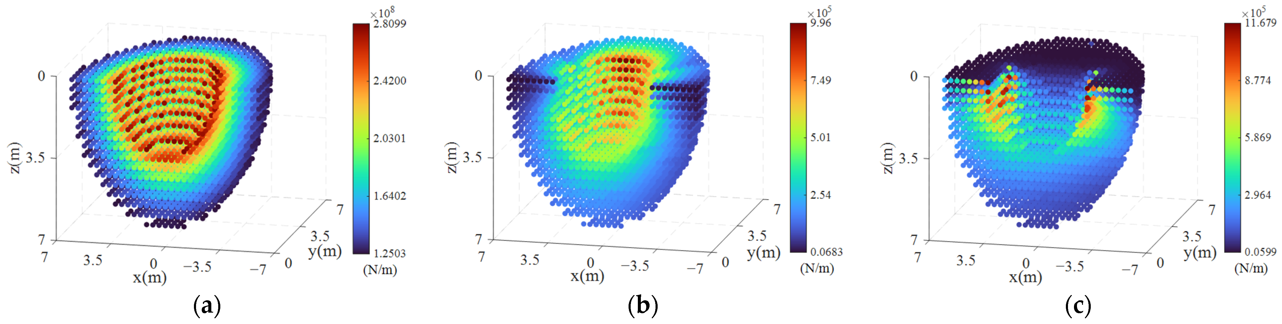
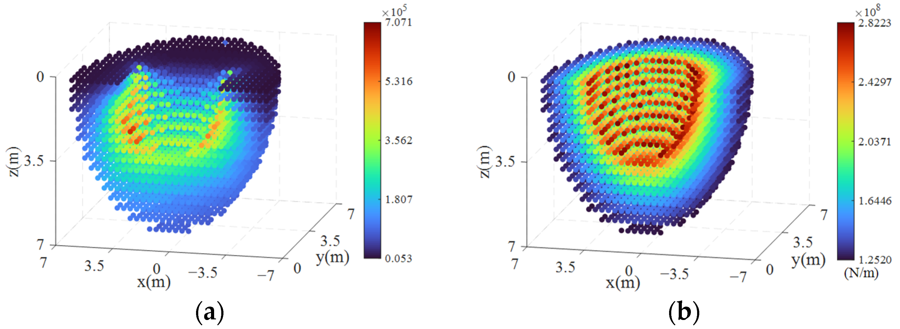
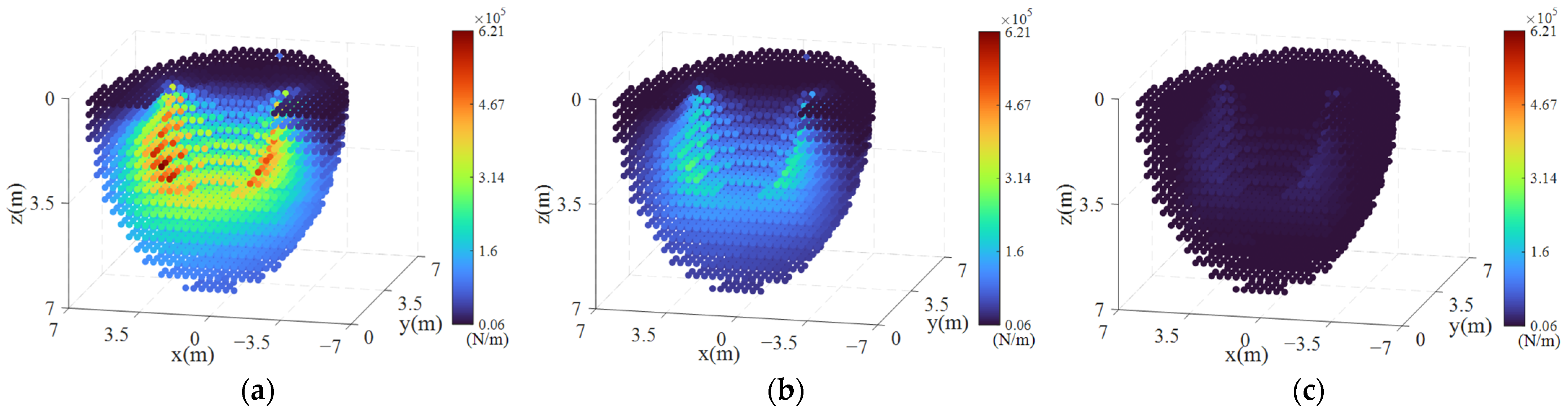
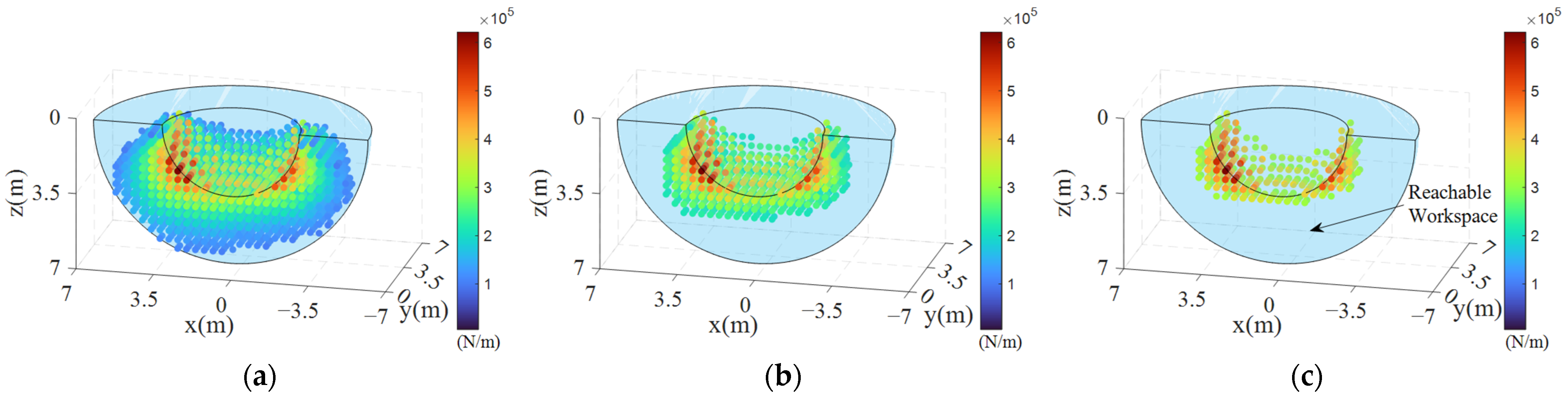
4.2.1. CDPR Stiffness Distribution

In practice, when controlling the CDPR end-effector to reach a specific point, the cables are first considered as elastic tension elements, and their theoretical lengths are calculated to meet geometric constraints. Next, the cable lengths are adjusted using cable-winding devices to achieve precise end-effector positioning. The reachable workspace of the CDPR is limited by the length of the telescopic rod, and theoretically, it is a hollow hemisphere. The subsequent stiffness analysis in the paper is based on this reachable workspace rather than the actual workspace used in engineering. We discretize the workspace into equidistant points and calculate the equilibrium state parameters of the CDPR system at these discrete points. The equilibrium equations employed are detailed in previous research [6], and the analysis parameters are provided in Table 2.
When analyzing CDPR stiffness, it is necessary to extract stiffness parameters with clear engineering significance. The derivation process follows the reference [20]. The stiffness in the j th direction in the global coordinate system is expressed as follows:
κ j = K j j k j K j 1 k j
where K j j is the element located in the j th row and j th column of the stiffness matrix K ; K j is the matrix K with the j th row and j th column removed; k j is the j th column of the matrix K with the j th element removed.
With a flight speed of 80 m/s, the three-direction stiffness (global coordinates) and the distribution of the minimum and maximum stiffness in the eigenvalues of the stiffness matrix of the CDPR are shown in Figure 9 and Figure 10. In the body coordinate system, due to the symmetry of the structure along the flight direction, the subsequent part of this paper only shows the analysis results of the +y-axis side.
From Figure 9a and Figure 10b, it can be seen that the distribution pattern and numerical values of the maximum stiffness align with those of the X -direction stiffness. This indicates that the CDPR system’s stiffness is greatest along the X -direction of the telescopic rod, with the X -direction stiffness primarily provided by the telescopic rod. Figure 9b,c show that the stiffness distribution in the Y and Z directions is uneven. This is mainly because the Y and Z direction stiffness is provided by the parallel cables, which is related to the layout of the cables in the CDPR. Figure 10a is particularly important as it illustrates the minimum stiffness distribution of the CDPR system within the reachable workspace. The minimum stiffness can be used to evaluate the overall strength of the CDPR system’s stiffness, which is significant for research on selecting interception areas and optimizing CDPR trajectories. The figure shows that when the z -coordinate value is relatively small, the CDPR system’s stiffness is lower. For points near the outer edges of the workspace, the system stiffness increases as the z -coordinate increases. The equilibrium points with higher stiffness are mainly found along the edges inside the workspace, particularly along the ± x -axis.

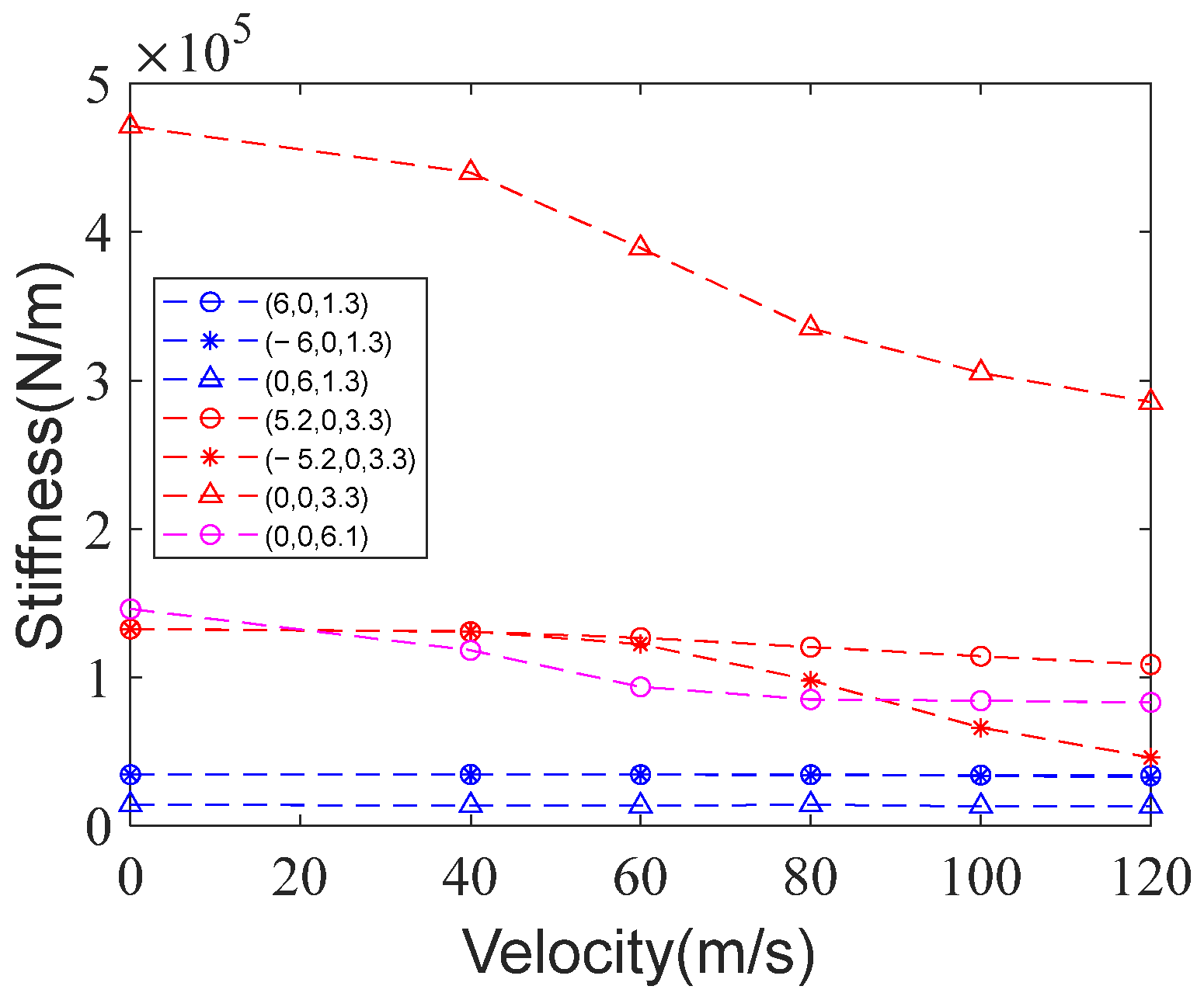
4.2.2. Influence of Flow Velocity on CDPR Stiffness

During the UAV’s aerial recovery operation, the flow velocity experienced by the CDPR matches the flight speed of the carrier aircraft. In the analysis, we vary the flow velocity and calculate the distribution of the minimum eigenvalues of the CDPR stiffness matrix accordingly.
From Figure 11, we observe that as the flow velocity increases, the overall distribution pattern of the CDPR stiffness within the workspace remains consistent, but the stiffness values decrease. To analyze the changes in stiffness values, we selected points at typical locations and plotted the stiffness variation curves at different positions as the flow velocity changes, as shown in the following Figure 12.
From Figure 12, it can be seen that as the flow velocity increases, the stiffness values exhibit a decreasing trend. Points with smaller stiffness values are located in the upper part of the workspace, such as points ( 6 , 0 , 1.3 ) , ( 6 , 0 , 1.3 ) , and ( 0 , 6 , 1.3 ) , where stiffness is less affected by changes in flow velocity. In contrast, points in the central part of the workspace, such as ( 5 . 2 , 0 , 3.3 ) , ( 5 . 2 , 0 , 3.3 ) , and ( 0 , 0 , 3.3 ) , and especially the near-center point ( 0 , 0 , 3.3 ) , have greater stiffness. Comparing the curves in Figure 12, we observe that points on the outer edges of the workspace show a decreasing trend in stiffness only when the flow velocity exceeds 60 m/s. In contrast, equilibrium points near the z-axis, such as ( 0 , 0 , 3.3 ) and ( 0 , 0 , 6 . 1 ) , are more sensitive to flow velocity changes, showing stiffness variations even at lower flow velocities. This is because the cables form a larger angle with the airflow direction, making them more prone to bending due to aerodynamic forces, as seen in previous single-cable stiffness analysis results.

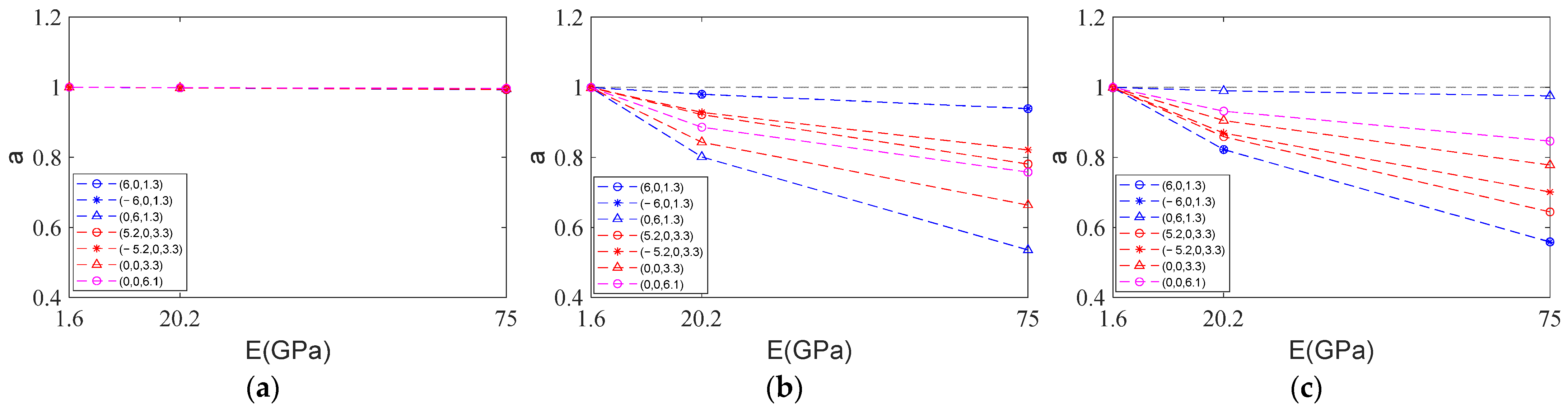
4.2.3. Influence of Different Cable Materials on CDPR Stiffness

In engineering applications, different materials are chosen for the cables in a CDPR system to meet control requirements, extend service life, or improve economic efficiency. However, the choice of cable material can impact the system’s stiffness. The following analysis examines the effect of different cable materials on the stiffness of the CDPR at a flight speed of 80 m/s.
Different cable materials have different elastic modulus. From Figure 13, it can be seen that as the material modulus decreases, the system stiffness shows a significant decreasing trend. When a low-modulus cable material is selected, the stiffness in each direction provided by the parallel cables is much lower compared to the axial stiffness of the telescopic rod. In such cases, we can simplify the expression of the CDPR stiffness matrix, as derived below. By considering the telescopic rod as a rod element, the 3 × 3 stiffness matrix K G P of the rod in the global coordinate system is as follows:
K G P = a 1 E A 3 l 4 a 1 + E A 3 0 0 0 0 0 0 0 0
For the four parallel cables, the relationship of the small forces at points B and P is as follows:
δ F C x P δ F C y P δ F C z P = δ F C x B 1 η δ F C y B 1 η δ F C z B = 1 0 0 0 1 η 0 0 0 1 η δ F C x B δ F C y B δ F C z B
The relationship of the small displacements at points B and P is as follows:
δ x C P δ y C P δ z C P = δ x C B η δ y C B η δ z C B = 1 0 0 0 η 0 0 0 η δ x C B δ y C B δ z C B
Combining Equations (13) and (14), we obtain the following:
δ F C x P δ F C y P δ F C z P = 1 0 0 0 1 η 0 0 0 1 η k 11 c k 12 c k 13 c k 21 c k 22 c k 23 c k 31 c k 32 c k 33 c 1 0 0 0 η 0 0 0 η 1 δ x C P δ y C P δ z C P
Further derivation leads to the stiffness expression as follows:
K C P = k 11 c 1 η k 12 c 1 η k 13 c 1 η k 21 c 1 η 2 k 22 c 1 η 2 k 23 c 1 η k 31 c 1 η 2 k 32 c 1 η 2 k 33 c
where η = A B A P , and combining the stiffness at point P gives us the overall system stiffness K P .
K P = K C P + K G P = a 1 E A 3 l 4 a 1 + E A 3 + k 11 c 1 η k 12 c 1 η k 13 c 1 η k 21 c 1 η 2 k 22 c 1 η 2 k 23 c 1 η k 31 c 1 η 2 k 32 c 1 η 2 k 33 c
Consequently, after assembly, we can see that the system stiffness in the X direction will approximate the axial stiffness of the telescopic rod, while the stiffness in the Y and Z directions will be proportional to the Y and Z stiffness of the parallel cables, with the proportionality factor depending on the spatial position of the CDPR.
At the typical positions mentioned earlier, we first calculate K P and K P . Then, we compute the three-directional stiffness values in the global coordinate system. We define the proportionality factor a i as the ratio of the stiffness values in the three directions.
a i = K P i K P i *
where i = 1 , 2 , 3 , represents the three directions in the global coordinate system. We then plot the curve of the proportionality factor a i as it varies with the elastic modulus of different cable materials.
From Figure 14, it can be seen that in the X direction, the two stiffness values are nearly equal. In the Y and Z directions, as the elastic modulus of the cable material decreases, the stiffness values tend to converge. This indicates that when there is a significant difference between the stiffness of the cables and the telescopic rod, a simpler stiffness expression can be used. This greatly reduces the complexity of calculating system stiffness.

4.3. Design Guidelines for the UAV Recovery System Based on Stiffness Analysis Results

Before capturing the UAV, the Cable-Driven Parallel Robot (CDPR) needs to make continuous, gradual adjustments to its position to ensure a successful interception. The previous analysis of stiffness distribution and influencing factors provides valuable insights that guide the design of the UAV recovery system.

4.3.1. Selection of the UAV Interception Spatial Position

Based on the previous analysis, the stiffness distribution of the CDPR system varies significantly across different working positions. When intercepting a UAV, it is crucial to select a working area with high system stiffness to enhance stability. Assuming the system stiffness needs to satisfy K P K l o w , where K l o w is the minimum required stiffness, the ideal interception spatial position for different K l o w values can be identified by referring to the system’s minimum stiffness distribution map (Figure 9), as shown in Figure 15.
As shown in Figure 15, as the minimum stiffness value K l o w increases, the working space decreases. The positions in Figure 13c, with their relatively high system stiffness, are advantageous for UAV recovery operations. Conducting the interception process in these areas can help minimize the impact of external disturbances and increase the success rate of the recovery process.

4.3.2. Selection of UAV Recovery Flight Speed

During UAV recovery, the aerodynamic load on the CDPR system increases with the carrier’s flight speed, directly affecting the overall stiffness of the system. Analysis results indicate that as airflow speed increases, system stiffness shows a significant downward trend. Therefore, a lower flight speed should be selected during UAV recovery to minimize the negative impact of aerodynamic loads on system stiffness. If the recovery mission must be conducted at high speeds, it is advisable to choose areas with higher system stiffness, such as positions near the inner edges of the working space.

4.3.3. Selection of Cable Material

The choice of cable material has a direct impact on the system’s stiffness. Analysis shows that using high-modulus materials (such as those with E = 75   GPa ) can significantly enhance system stiffness, particularly in the Y and Z directions provided by the parallel cables. Therefore, when designing the UAV recovery system, high-modulus materials should be prioritized to improve the overall rigidity of the system.

5. Conclusions

This paper analyzes the CDPR stiffness problem for UAV aerial recovery systems in a flow field environment. Starting from the cable model established in previous studies, a solution for the stiffness of the spatial cable considering aerodynamic loads is provided. The analysis of the spatial cable’s equilibrium position and stiffness reveals that aerodynamic loads significantly affect the cable’s stiffness, and this effect is related to the angle between the cable and the direction of the flow field. The stiffness matrices of the system’s individual elements were analyzed, and the CDPR system stiffness was assembled using the finite element method. Simulation analysis provided the spatial distribution of the CDPR system stiffness, which is symmetrical along the flight longitudinal plane. The maximum stiffness occurs in the central region of the workspace. The effects of flow speed and cable material on system stiffness were analyzed. As the flow field speed increases, the system stiffness decreases, with the central position being more significantly affected by the flow speed. As the elastic modulus of the materials decreases, the system stiffness also shows a noticeable decline. The final derivation provides a simplified stiffness expression for cases where the cable stiffness is much lower than the stiffness of the telescopic rod. In conclusion, the stiffness analysis results provide valuable design guidance for the CDPR system. The results of this study provide a theoretical basis for stiffness analysis in cable-driven UAV aerial recovery systems, offering theoretical tools for system design and optimization. Additionally, it provides methods for analyzing the stiffness of CDPRs in flow fields.

Author Contributions

Conceptualization, methodology, validation, formal analysis, J.W. and H.Y.; software, investigation, X.P. and Y.Z.; resources, H.Y.; data curation, writing—original draft preparation, J.W., F.Y. and Y.W.; writing—review and editing, J.W.; visualization, X.P. and Y.Z.; project administration, funding acquisition, H.Y. All authors have read and agreed to the published version of the manuscript.

Funding

This research was funded by the Foundation of Chinese State Key Laboratory of Robotics and Systems (Grant No. SKLRS202203B) and the China Postdoctoral Science Foundation (Grant No. GZB20240955).

Data Availability Statement

Data are contained within the article.

Conflicts of Interest

The authors declare no conflicts of interest.

References

  1. Liu, Y.H.; Wang, H.L.; Fan, J.X.; Wang, Y.X.; Wu, J.F. Trajectory stabilization control for aerial recovery of cable-drogue-UAV assembly. Nonlinear Dyn. 2021, 105, 3191–3210. [Google Scholar] [CrossRef]
  2. Choi, A.J.; Yang, H.H.; Han, J.H. Study on robust aerial docking mechanism with deep learning based drogue detection and docking. Mech. Syst. Signal Process. 2021, 154, 107579. [Google Scholar] [CrossRef]
  3. Su, Z.K.; Li, C.T.; Liu, Y.H. Anti-disturbance dynamic surface trajectory stabilization for the towed aerial recovery drogue under unknown airflow disturbances. Mech. Syst. Signal Process. 2021, 150, 107342. [Google Scholar] [CrossRef]
  4. Liu, Y.; Qi, N.; Yao, W.; Zhao, J.; Xu, S. Cooperative Path Planning for Aerial Recovery of a UAV Swarm Using Genetic Algorithm and Homotopic Approach. Appl. Sci. 2020, 10, 4154. [Google Scholar] [CrossRef]
  5. Voskuijl, M.; Said, M.R.; Pandher, J.; Tooren, M.J.V.; Richards, B. In-flight deployment of morphing UAVs—A method to analyze dynamic stability, controllability and loads. In Proceedings of the AIAA Aviation 2019 Forum, Dallas, TX, USA, 17–21 June 2019. [Google Scholar]
  6. Wu, J.; Sun, Y.; Yue, H.; Yang, J.; Yang, F.; Zhao, Y. Design and Optimization of UAV Aerial Recovery System Based on Cable-Driven Parallel Robot. Biomimetics 2024, 9, 111. [Google Scholar] [CrossRef] [PubMed]
  7. Zarebidoki, M.; Dhupia, J.S.; Xu, W. A Review of Cable-Driven Parallel Robots: Typical Configurations, Analysis Techniques, and Control Methods. IEEE Robot. Autom. Mag. 2022, 29, 89–106. [Google Scholar] [CrossRef]
  8. Qian, S.; Zi, B.; Shang, W.-W.; Xu, Q.-S. A Review on Cable-driven Parallel Robots. Chin. J. Mech. Eng. 2018, 31, 66. [Google Scholar] [CrossRef]
  9. Zhang, Z.; Shao, Z.; You, Z.; Tang, X.; Zi, B.; Yang, G.; Gosselin, C.; Caro, S. State-of-the-art on theories and applications of cable-driven parallel robots. Front. Mech. Eng. 2022, 17, 37. [Google Scholar] [CrossRef]
  10. Kawamura, S.; Kino, H.; Won, C. High-speed manipulation by using parallel wire-driven robots. Robotica 2000, 18, 13–21. [Google Scholar] [CrossRef]
  11. Cui, Z.; Tang, X. Analysis of stiffness controllability of a redundant cable-driven parallel robot based on its configuration. Mechatronics 2021, 75, 102519. [Google Scholar] [CrossRef]
  12. Cui, Z.; Tang, X.; Hou, S.; Sun, H. Research on Controllable Stiffness of Redundant Cable-Driven Parallel Robots. IEEE/ASME Trans. Mechatron. 2018, 23, 2390–2401. [Google Scholar] [CrossRef]
  13. Gueners, D.; Chanal, H.; Bouzgarrou, B.C. Stiffness optimization of a cable driven parallel robot for additive manufacturing. In Proceedings of the IEEE International Conference on Robotics and Automation (ICRA), Paris, France, 31 May–31 August 2020; pp. 843–849. [Google Scholar]
  14. Max Irvine, H. CABLE Structures; MIT Press: Cambridge, MA, USA, 1981. [Google Scholar]
  15. Merlet, J.P. A generic numerical continuation scheme for solving the direct kinematics of cable-driven parallel robot with deformable cables. In Proceedings of the 2016 IEEE/RSJ International Conference on Intelligent Robots and Systems (IROS), Daejeon, Republic of Korea, 9–14 October 2016; pp. 4337–4343. [Google Scholar]
  16. Yuan, H.; Courteille, E.; Deblaise, D. Static and dynamic stiffness analyses of cable-driven parallel robots with non-negligible cable mass and elasticity. Mech. Mach. Theory 2015, 85, 64–81. [Google Scholar] [CrossRef]
  17. Jung, J. Workspace and Stiffness Analysis of 3D Printing Cable-Driven Parallel Robot with a Retractable Beam-Type End-Effector. Robotics 2020, 9, 65. [Google Scholar] [CrossRef]
  18. Gao, T.; Wang, Q.; Wang, J.; Su, Y.; Tian, J.; Wu, S. Overall stiffness derivation and enhancement algorithm of a flying cable-driven parallel robot. J. Mech. Sci. Technol. 2024, 38, 873–884. [Google Scholar] [CrossRef]
  19. Nagarajan, P. Matrix Methods of Structural Analysis, 1st ed.; CRC Press: Boca Raton, FA, USA, 2018; pp. 193–313. [Google Scholar]
  20. Arsenault, M. Workspace and stiffness analysis of a three-degree-of-freedom spatial cable-suspended parallel mechanism while considering cable mass. Mech. Mach. Theory 2013, 66, 1–13. [Google Scholar] [CrossRef]
  21. Yuan, H.; Courteille, E.; Deblaise, D. Eastodynamic Analysis of Cable-Driven Parallel Manipulators Considering Dynamic Stiffness of Sagging Cables. In Proceedings of the 2014 IEEE International Conference on Robotics and Automation (ICRA), Hong Kong, China, 31 May–7 June 2014; pp. 4055–4060. [Google Scholar]
Figure 1. UAV aerial recovery system based on CDPR.
Actuators 13 00343 g001
Figure 2. Static equilibrium force analysis of the cable.
Actuators 13 00343 g002
Figure 3. The CDPR configuration for UAV recovery system.
Actuators 13 00343 g003
Figure 4. The elements and nodes of the CDPR.
Actuators 13 00343 g004
Figure 5. The local coordinate system of element 5.
Actuators 13 00343 g005
Figure 6. Distribution of the spatial equilibrium positions of point B under different conditions: (a) Three-dimensional view; (b) x-direction view; (c) y-direction view; (d) z-direction view.
Actuators 13 00343 g006
Figure 7. Distribution of the cable bending degree λ : (a) Considering mass and elasticity; (b) considering mass, elasticity, and aerodynamic loads.
Actuators 13 00343 g007
Figure 8. Maximum stiffness distribution of the cable: (a) Considering mass and elasticity; (b) considering mass, elasticity, and aerodynamic loads.
Actuators 13 00343 g008
Figure 9. CDPR stiffness in three directions: (a) X -direction; (b) Y -direction; (c) Z -direction.
Actuators 13 00343 g009
Figure 10. CDPR minimum and maximum stiffness distribution: (a) Minimum stiffness; (b) maximum stiffness.
Actuators 13 00343 g010
Figure 11. Stiffness distribution under different flow velocities: (a) 0 m/s; (b) 40 m/s; (c) 60 m/s; (d) 80 m/s; (e) 100 m/s; (f) 120 m/s.
Actuators 13 00343 g011
Figure 12. Stiffness variation curves of typical points with changing flow velocity.
Actuators 13 00343 g012
Figure 13. Stiffness distribution corresponding to different cable materials: (a) E = 75 GPa; (b) E = 20.2 GPa; (c) E = 1.6 GPa.
Actuators 13 00343 g013
Figure 14. The a i values corresponding to the different cable materials: (a) X -direction; (b) Y -direction; (c) Z -direction.
Actuators 13 00343 g014
Figure 15. The ideal interception spatial position for different K l o w values: (a) K l o w = 100,000 N / m ; (b) K l o w = 200,000 N / m ; (c) K l o w = 300,000 N / m .
Actuators 13 00343 g015
Table 1. Parameter name and parameter symbol.
Parameter NameParameter Symbol
Spatial coordinates of endpoint B ( B x , B y , B z )
The tension at endpoint B ( t B x , t B y , t B z )
Cable free length L 0
Young’s modulus of the cable E
Cable cross-sectional area A
Cable diameter D
The aerodynamic forces per unit length ( k x , k y , k z )
Cable density ρ c
Gravity acceleration g
Air density at 3 km altitude ρ a
Aerodynamic friction coefficient c t
Aerodynamic drag coefficient c n
The airflow velocity ( v x , v y , v z )
Intermediate variables a 1 , a 2 , a 3 , b 1 , b 2 , b 3
Table 2. The structural and aerodynamic parameters for the CDPR.
Parameter NameParameter SymbolValue
Cable diameter D 0.01   m
Cable cross-sectional area A 7.854 × 10 5 m 2
Young’s modulus E 75   GPa
Cable density ρ c 999 . 5   kg / m 3
Span 1 d 1 4   m
Span 2 d 2 3   m
Telescopic rod weight m 122   kg
Telescopic rod diameter L 1 2   m
Telescopic rod elongation length L 2 , L 3 1 2 ( AB L 1 )
Telescopic rod shortening length OP min 3.12   m
Telescopic rod elongation length OP max 6.22   m
Axial stiffness of the telescopic rod k g 5 × 10 7 N / m
Air density at 3 km altitude ρ a 0 . 9096   kg / m 3
Aerodynamic friction coefficient c t 0.02
Aerodynamic drag coefficient c n 0.8
Carrier aircraft flight speed v 80   m / s
Gravity acceleration g 9 . 8   m / s 2
Disclaimer/Publisher’s Note: The statements, opinions and data contained in all publications are solely those of the individual author(s) and contributor(s) and not of MDPI and/or the editor(s). MDPI and/or the editor(s) disclaim responsibility for any injury to people or property resulting from any ideas, methods, instructions or products referred to in the content.

