Abstract
This paper presents the modeling and control of a flexible single-boom crane manipulator using a high-fidelity real-time simulation model. The model incorporates both electro-hydraulic actuation and flexible-body dynamics, with the flexible boom represented via the lumped parameter method. A systematic tuning and validation procedure ensures that the model accurately replicates the physical system’s dynamics, achieving an eigenfrequency accuracy of approximately 97% and a piston-position deviation within 1.2% of the overall stroke length in final tests. The real-time simulation model is utilized in both open-loop and closed-loop control schemes to investigate whether simulated data can reduce dependency on sensor feedback compared to a benchmark controller. While the simulation-based controller alone does not match the fully sensor-based closed-loop accuracy, the simulation-based feedforward improves performance by 83% compared to the standard model-based velocity feedforward. Additionally, integrating the real-time simulation with sensor feedback enhances the benchmark controller’s performance by approximately 16%. These findings highlight the potential of combining real-time, nonlinear simulation with conventional sensor feedback to enhance the control of electro-hydraulic flexible manipulators.
1. Introduction
The increasing prevalence of autonomous applications in industry has driven the demand for more accurate and robust control systems. Traditional robotic manipulators often rely on rigid, high-stiffness structures to minimize vibration and improve positional accuracy. Although effective in some contexts, these designs compromise both energy efficiency and speed relative to payload capacity [1]. In contrast, modern industrial and robotic applications increasingly favor lightweight manipulators, which offer advantages such as reduced cost, improved payload-to-weight ratio, increased operational speed, and enhanced energy efficiency and safety due to lower inertia [1,2,3]. However, these benefits come at the expense of increased structural flexibility, leading to deflections and oscillations that complicate control, particularly in hydraulic systems, which already exhibit complex nonlinear behavior [4].
Hydraulic actuation remains a preferred choice in various industries due to its high power density and force capabilities. However, hydraulic systems introduce additional control challenges that stem from nonlinear dynamics, volumetric and hydromechanical losses, compressibility effects, and frictional interactions [5,6,7]. Although tools like MATLAB Simulink and its libraries offer convenient solutions for modeling hydraulics and electromechanical systems [6], these built-in physical models are not optimized for real-time performance. This requires the development of custom models to enable real-time operation on industrial PCs (IPCs), which is essential for applications in control design, predictive maintenance, and system optimization.
Significant progress has been made in fault detection and predictive maintenance of electric drives and gearboxes [8,9,10]. However, fewer studies have explored combined electro-hydraulic and flexible-link systems, despite their critical role in industrial and robotic applications. Real-time high-fidelity simulation models that capture the coupled mechanical, hydraulic, and electrical dynamics of these systems are essential to advance control strategies, diagnostics, and maintenance protocols.
Several advances have been made in the efficient modeling of hydraulically actuated systems to address fundamental challenges, including the compressibility of the hydraulic fluid, the flexibility of the mechanical structure, the friction in hydraulic actuators, and the dynamics of control elements. The latter may include, i.e., the spool position of a servo valve, the swash plate angle of a variable displacement pump, or, in the case of direct-drive actuators, the angular velocity of a servo motor acting as the primary mover. Achieving real-time simulation accuracy within computational constraints requires a well-defined accuracy target and an optimal balance between model complexity and parameter selection.
Mechanical systems comprising multiple bodies can lead to computationally expensive simulations, particularly in the presence of closed kinematic loops. However, the use of screw theory, as presented in [11], offers an efficient approach to mitigating this challenge for hydraulically actuated systems. Another key difficulty lies in accurately capturing the compressibility effects of hydraulic fluids. A real-time model presented in [12] successfully addresses this problem while also incorporating cylinder friction and controller dynamics. However, it assumes a constant bulk modulus, which is a reasonable approximation at high pressure levels but is not suitable for direct-drive applications where fluid compressibility varies.
In this work, we develop a real-time simulation model of a hydraulically actuated system featuring a mechanically flexible structure. The model explicitly accounts for variable fluid compressibility and cylinder friction, capturing essential nonlinearities in the coupled electro-hydraulic–mechanical dynamics. To address the computational challenges associated with real-time performance, we adopt a lumped parameter modeling approach, which balances efficiency and accuracy in flexible link simulations [2,13].
Although accurate modeling is critical, achieving effective control of such systems presents additional challenges. Industrial control systems often rely on Proportional–Integral–Derivative (PID) controllers due to their simplicity and robustness [14]. However, given the complex dynamics of flexible hydraulic systems, advanced model-based strategies, such as feedforward control, are necessary to improve disturbance rejection and control precision [15,16]. Integrating simulation-derived and sensor-derived data further improves the robustness and adaptability of the system under uncertain operating conditions [17,18].
To validate these modeling and control strategies, we investigate a single-boom crane actuated by a Self-Contained Electro-Hydraulic Cylinder (SCC). The crane, located in the Norwegian Motion Laboratory (https://www.uia.no/motionlab, accessed on 30 December 2024) at the University of Agder, features a slender, flexible boom that exhibits significant mechanical and hydraulic oscillations. These dynamic interactions present unique challenges for precise control. By formulating and validating a high-fidelity real-time simulation model and deploying it within both open-loop and closed-loop control frameworks, this study aims to address fundamental challenges in flexibility and nonlinear hydraulic behavior for crane and manipulator systems. The main contributions of this paper are:
- Development and deployment of a high-fidelity real-time simulation model that integrates lumped parameter modeling of the flexible boom with accurate hydraulic system dynamics.
- Introduction of a simulation-based control framework that enables effective open-loop and closed-loop control strategies.
- Rigorous validation of the simulation model through eigenfrequency matching, experimental testing, and parametric tuning to ensure dynamic fidelity.
- Investigation of boom-induced pressure oscillations and their impact on control performance.
- Comparative evaluation against a benchmark control system, highlighting the advantages and limitations of simulation-based strategies.
- Provision of methodologies and insights applicable to broader industrial systems, including lightweight robotic manipulators and energy-efficient hydraulic actuation systems.
2. System Overview
This section outlines the electro-hydraulically actuated flexible crane considered in this work. All key structural parameters and component parameters have been derived from a combination of experimental measurements, manufacturer datasheets, and literature references (e.g., [19,20,21]). The precision of these parameters has been validated in previous studies and forms the basis for our modeling and control design.
As shown in Figure 1, the setup considered comprises a single boom crane driven by the SCC. Located in the UiA Motion Lab, the system serves as a testbed representing various load-carrying applications. A benchmark controller is introduced to compare its performance with the proposed simulation-based approach.
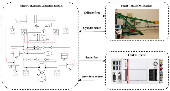
Figure 1.
Overview of the electro-hydraulically actuated flexible crane. The mechanical system (a single boom with a fixed payload), the self-contained electro-hydraulic actuator, and the Beckhoff real-time control system are highlighted.
2.1. Flexible Boom Mechanism
The crane has a -long boom that carries a payload at its tip. As illustrated in Figure 1, the boom pivots on a bearing on the base and is actuated by a double-acting hydraulic cylinder connected to the boom and the base through two additional revolute joints. This long and lightweight design introduces significant structural flexibility, which has been characterized by experimental measurements in our lab. Figure 2 shows the main kinematic dimensions of the crane. The distance from the bearing (A) to the combined boom–payload center of mass (G) is , and the total mass is . The effective length of the hydraulic cylinder, , connecting points B and C varies between and , depending on the piston travel, . Table 1 summarizes these and other parameters. Although earlier studies derived crane dynamics using a Lagrangian approach, this work employs a lumped parameter model to capture the essential flexibility of the boom and its interaction with the hydraulic system (see Section 3).
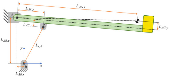
Figure 2.
Kinematic representation of the single-boom crane. Key dimensions and coordinates are indicated.

Table 1.
Key parameters of the crane mechanism.
2.2. Electro-Hydraulic Actuation System
A simplified SCC schematic, detailed in [20], is shown in Figure 3, with the numbered components listed in Table 2. Five pressure transducers (one for each modeled pressure) and a position sensor track the cylinder piston displacement. The red dotted lines represent the pilot lines.
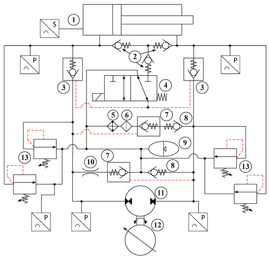
Figure 3.
Simplified electro-hydraulic circuit of the SCC, incorporating five pressure sensors (P) and a piston position sensor (S). The numbered components correspond to those listed in Table 2 while the red dotted lines represent the pilot lines.
Table 2.
System components of the self-contained electro-hydraulic actuation system.
The actuation system uses a double-acting asymmetric cylinder with a diameter of the piston and a diameter of the rod . An Axial Piston Machine (APM) with fixed displacement () is driven by a Servo Motor (SM) to provide bidirectional flow. By eliminating proportional/servo valves and directly controlling the flow via the speed and direction of the SM, the SCC achieves higher energy efficiency by significantly reducing throttling losses compared to conventional valve control.
A 3/2 Directional Control Valve (DCV) supports load holding when the valve is energized the higher pressure on either the piston side or rod side pilots the pilot-operated check valves (3) open. When deenergized, the accumulator side provides low pilot pressure, closing the check valves, and securely holding the load pressure.
2.3. Control System
Figure 4 outlines the real-time control system, featuring a Bosch Rexroth servo drive, a Bosch Rexroth Remote I/O module, the Beckhoff IPC, and a development PC running MATLAB Simulink and TwinCAT 3 Engineering. EtherCAT ensures high-speed, real-time, deterministic communication, while standard Ethernet handles software development and supervisory tasks.
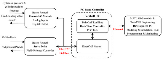
Figure 4.
Control system architecture for real-time operation.
The servo drive applies Field-Oriented Control (FOC) for precise regulation of the SM’s speed and torque. Feedback signals from the SM (e.g., position, velocity) are used to close the control loop. Meanwhile, the CX2043 IPC (manufactured by Beckhoff Automation GmbH & Co. KG, Verl, Germany) with an AMD Ryzen™ V1807B CPU at 3.35 GHz runs the TwinCAT runtime for Programmable Logic Controller (PLC) tasks. This embedded IPC supports cycle times in the microsecond range on individual CPU cores, making it suitable for computationally intensive tasks such as real-time simulation and advanced control.
A separate development PC handles modeling, code generation, and supervisory functions, communicating with the IPC over Ethernet. MATLAB Simulink and TwinCAT engineering tools enable seamless workflow transitions, from model-based design to runtime deployment.
2.3.1. Benchmark Controller
A benchmark controller, as shown in Figure 5, was developed in [20] and is used to evaluate the simulation-based control proposed in this paper.
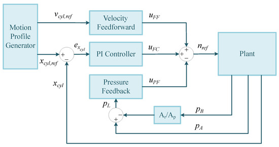
Figure 5.
Benchmark controller architecture.
The benchmark controller regulates the SM speed according to the reference signal . It comprises a velocity feedforward , a PI controller , and active damping through load pressure feedback.
The velocity feedforward term is calculated as follows:
where is the piston area, is the desired piston velocity, and is the flow gain that relates the pump flow to the SM speed. The factor of 60 converts to rpm.
A standard PI controller produces the feedback control signal:
where is the position error, is the proportional gain, and is the integral gain.
Active damping attenuates oscillations by using load pressure . The damping term is as follows:
where is derived from the pressures of the piston and rod side, and define the high-pass filter, and is the flow gain.
3. System Modeling
This section outlines the physical principles and mathematical formulations used to model the electro-hydraulically actuated flexible crane boom introduced in Section 2. The modeling process starts with the electro-hydraulic actuation system, which determines the hydraulic cylinder force that interacts with the flexible boom mechanism (see Figure 1) and culminates in the derivation of the combined system dynamics that is implemented on the Beckhoff IPC in Section 5 to allow real-time simulation. The internal dynamics of the SM are omitted because its response is significantly faster than that of the hydraulic system.
3.1. Electro-Hydraulic Actuation System
This section describes the equations of the hydraulic model, starting with the definition of pressure nodes and the locations of volume flows through resistances. Figure 6 highlights the five pressure nodes () and the flow directions in the system.
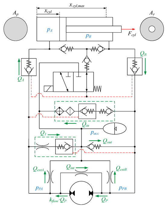
Figure 6.
Hydraulic schematic showing pressure nodes and flow definitions.
The schematic excludes pressure relief valves (assumed to be normally closed), while internal pump leakage and accumulator outflow are modeled as orifices. The DCV is treated as a logic switch, and the check valves and the cooler are omitted. The positive directions for the position of the piston, the external force, and the volume flows are defined in Figure 6, with the pilot lines shown as red dotted lines.
Two regions with multiple orifices in series, marked by green dotted boxes in Figure 6, are simplified as effective resistances by assuming small valve volumes. This reduces the number of pressure gradients to compute and avoids stiff liquid volumes that require small simulation time steps.
3.1.1. Volume Flows
Volume flow rates through the valves, as illustrated in Figure 7, are governed by the orifice equation as follows:
where may be constant or variable, depending on the type of valve, and is the pressure difference across the valve. For valves with a variable opening (for example, check valves or directional control valves), is a function of the dimensionless opening of the valve. For constant valves such as a throttle valve, remains fixed.
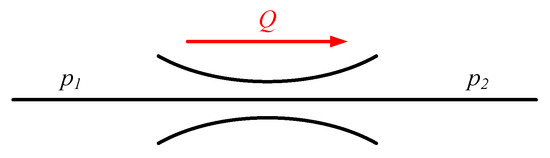
Figure 7.
Flow through an orifice.
The flow of the APM is described by the following:
where n is the SM speed and is the displacement of the APM.
The valve flows, as shown in Figure 6, are detailed in Appendix A.1. These include internal leakage, case drain flows, flows through check valves, effective valve constants, and specific path flows such as and .
3.1.2. Pressure Dynamics
Figure 6 defines five pressure nodes in the system, resulting in five pressure gradient equations. The pressure dynamics for a Newtonian fluid, which approximates hydraulic oil behavior, are governed by:
where is the effective stiffness of the oil, V is the volume of the pressure node, is the rate of change in volume, and is the net flow entering or exiting the node. The flow directions follow the conventions in Figure 6.
The effective bulk modulus, , describes the relationship between pressure changes and fluid compressibility. It plays a crucial role in hydraulic systems as it influences their dynamic behavior and efficiency. The variation of as a function of pressure is illustrated in Figure 8.
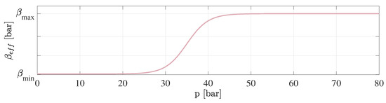
Figure 8.
Effective hydraulic oil bulk modulus as a function of pressure.
This influence is especially pronounced at low pressure levels, and it has been necessary to operate with a variable bulk modulus in this work to mirror the measured behavior satisfactorily. This relationship has been modeled using a hyperbolic tangent function:
To address the nonlinear nature of , the flow gain is computed numerically. For the constant case, where , the computed value of is 0.995. In contrast, for the variable case, with , , , and , the value of is 0.91. For both cases, the pressure difference is set at 80 bar.
The pressure gradient equations for the nodes associated with the inlet and outlet of the APM are as follows:
where and represent the effective oil stiffness for the respective nodes, and are their respective volumes, and is the flow gain. Since the flow goes to the pressure node , the constant is multiplied by .
The pressure gradients for the remaining nodes and account for the dynamics of the cylinder and the accumulator, including the effects of flow rates, volume changes due to piston movement, and total volume conservation governed by the polytropic gas law. Detailed derivations and associated equations are provided in Appendix A.2.
3.1.3. Cylinder Force
The cylinder force is determined as
where is the hydraulic force due to the pressure differential across the cylinder chambers, and is the friction force.
The hydraulic force is expressed as
where is the piston area, is the rod side ring area (annulus), as illustrated in Figure 6, and and are the pressures on the sides of the piston and rod, respectively.
The friction force is modeled using the modified Stribeck friction model:
where is the viscous friction coefficient, is the Coulomb friction force, is the static friction force, is the static friction constant, is the velocity of the cylinder, and a is a tuning parameter.
This approach, adapted from Padovani et al. [20], ensures numerical smoothness but introduces the limitation of zero friction at zero velocity.
3.2. Flexible Boom Mechanism
Modeling a flexible boom mechanism requires meeting specific criteria to ensure an accurate representation of the physical system. Three key factors are:
- Eigenfrequency: to ensure that the correct stiffness and effective mass are used to accurately replicate the system's oscillatory behavior and dynamics.
- Damping: to incorporate the correct structural damping to capture energy dissipation in the system effectively.
- Kinetics: to use accurate inertia data to reflect the system's dynamic behavior and interactions.
In theoretical models, the eigenfrequency often exceeds that of the physical system because the flexibility is underestimated. To address this without adding complexity, the effective Young’s modulus (E) in the model is reduced. This adjustment reduces stiffness and fine-tunes the eigenfrequency to match the physical system, as further detailed in Section 5.2.2.
3.2.1. Lumped Parameter Modeling
The lumped parameter method, also known as the finite segment method, was used to model the flexible boom mechanism in [21,22]. This method represents the beam as several shorter segments connected by revolute joints, with each joint incorporating a torsional spring-damper system. The stiffness and damping coefficients, and , are derived from the geometry of the beam and the material properties and are calculated as follows [21,22]:
where E is the Young modulus, I is the second moment of the cross-section area of the segment, is the length of the segment, is the damping ratio, and is the mass moment of inertia of the segment.
In [21], the model was developed using SimulationX, while in [22], MATLAB Simulink Simscape Multibody was used to create a high-fidelity version. Both implementations accurately captured the flexibility of the system. However, due to the computational demands of the high-fidelity model, it was unsuitable for real-time applications, necessitating the development of a simplified version.
The high-fidelity models described in [21,22] divided the boom into 10 segments, with five segments between points A and C and five between point C and the payload. For real-time applications, these models were redesigned by reducing the segments from 10 to 3, balancing computational cost and accuracy. The simplified model focuses on replicating the eigenfrequency of the physical system rather than achieving precise tool-point accuracy, as the primary goal is to capture the dynamic behavior of the boom and its effect on the hydraulic system. The proposed lumped model is illustrated in Figure 9, showing three rigid bodies connected by revolute joints and torsional springs.
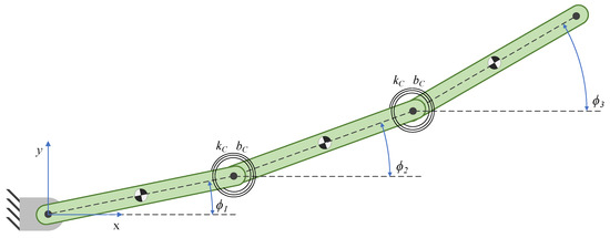
Figure 9.
The simplified lumped parameter model with three segments.
The torsional spring and damper torques between the lumped segments, which account for the boom stiffness, are computed as follows:
where , , and represent the angular positions of the three bodies, while , , and are their respective angular velocities. The coefficients and are given by Equations (13) and (14).
3.2.2. Dynamics
The lumped-parameter method models the single boom as a system of three interconnected rigid bodies. Figure 10 illustrates the derived system, including the vector notation used in the dynamic equations. This model is built on the principles of rigid body dynamics and Newtonian mechanics. The process involves solving moment-equilibrium equations to determine the angular acceleration of each body in the system.
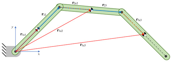
Figure 10.
The multibody system derived using the lumped parameter method.
Once the angular accelerations are calculated, they are integrated over time to update the positions and velocities of each body, ensuring an accurate representation of the system’s motion.
The forward kinematics of the system is found using the angular position vector, , derived in Equation (32). Kinematics is calculated using basic trigonometry, providing the positions of key points in each body, such as the mass center’s positions in the global coordinate system:
The equations of motion are derived using Free Body Diagrams (FBD) and Kinetic Diagrams (KD) for the third segment, the second and third segments, and the three segments. These diagrams are used to establish the relationships between the forces and moments acting on the bodies.
The initial dynamic analysis for body 3, as well as for bodies 2 and 3, has been relocated to Appendix B. The dynamic analysis for all three bodies is presented in the following, followed by the derivation of the cylinder force dynamics and the calculation of angular accelerations.
Dynamic Analysis for All Three Bodies
The dynamics of all three bodies are then analyzed collectively, as shown in Figure 11. This provides a complete representation of the system.
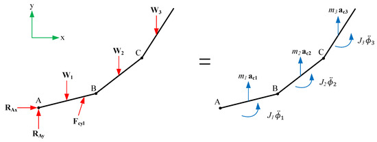
Figure 11.
Free body diagram and kinetic diagram for the three lumped segments.
To derive the equations of motion, the moments around point A from the force diagram are equated to the moments around point A from the kinetic diagram, resulting in the following:
Here, the cylinder force , which contributes to the system’s moments, is derived from Equation (10). In general, the hat symbol (^) indicates that it is the perpendicular vector, obtained by rotating the original vector counterclockwise. The linear accelerations of the center of mass of the three bodies are defined as
incorporating the angular accelerations and velocities of the connected segments.
The equations of motion for all three bodies are then assembled into a system of three moment equations with three unknowns:
The vector of applied moment, , captures the moments of the torsional spring, damper torques, gravitational forces, and the moment of the cylinder force about point A. The coefficient matrix, , contains terms related to angular accelerations. The system of dynamic equations is expressed as follows:
where the applied moment vector is
and the components are defined as
where , , and represent only the terms dependent on the angular velocity of Equations (19), (20), and (21), respectively. The detailed derivation of these equations can be found in Appendix B.
The coefficient matrix is defined as
where the terms are as follows:
Dynamics of Cylinder Force and Relative Position Vectors
The moment arm of the cylinder force, , and the relative position vector, , which are critical to the system dynamics, are illustrated in Figure 12. The vector represents the position of the cylinder mount (C) relative to the fixed point (A), while represents the relative position between the cylinder mount (C) and the fixed attachment point on the base of the cylinder (B). These vectors provide the geometric basis for computing the forces and motions within the system.
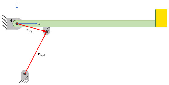
Figure 12.
Illustration of the moment arm of the cylinder force, , and the relative position vector, . The fixed attachment point (A), the base attachment point (B), and the cylinder mount (C) are highlighted.
The displacement and extension rate of the cylinder are given by
where represents the piston travel and describes the rate of extension (velocity) along the cylinder axis.
The fixed attachment point of the base of the cylinder is located at along the x direction and along the y direction, as illustrated in Figure 2 and detailed in Table 1. The parameter denotes the length of the cylinder when fully retracted, serving as a reference for calculating both the displacement of the cylinder and the extension velocity.
Iterative Calculation of Angular Acceleration, Velocity, and Position
The angular acceleration vector is calculated as
The angular velocity vector and the angular position vector are the state vectors of the mechanical system and are updated according to:
where and represent the angular velocity and angular position vectors of the system, respectively. Each vector comprises the angular velocity or position components of all the bodies in the system:
where and are the angular velocity and acceleration of the first body, and are those of the second body, and so on.
4. Simulation-Based Control Design
This section is devoted to the integration of the real-time simulation model in the control strategy of the physical system. Two distinct control strategies are implemented and tested: an open-loop control based solely on the simulation model and a closed-loop control that combines sensor feedback with simulation-based feedforward. The primary objectives are:
- Investigate whether real-time simulation can reduce the dependency on sensor feedback.
- Assess whether simulation-based feedforward improves position tracking in closed-loop control.
4.1. Open-Loop Control
The first approach is an open-loop controller that computes the control input using only the state of the real-time simulation model, without any sensor feedback from the physical system. Figure 13 illustrates this setup, where the position reference and the velocity reference are fed into the simulation model. The model outputs the input control signal , which then drives the motor.
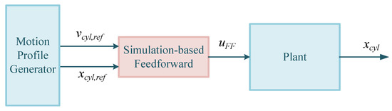
Figure 13.
Open-loop simulation-based feedforward control.
Figure 14 shows the internal structure of the simulation-based feedforward. It applies the same benchmark control system (Section 2.3.1) to the simulation model, using simulated signals , , and as feedback. The resulting control signal is then used in the physical configuration.
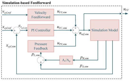
Figure 14.
Benchmark control system implemented on the simulated model.
Within this control system, the velocity feedforward is defined by
where is given in mm/s and in rpm.
The PI controller follows the standard proportional–integral structure:
where and are tuned in simulation. Table 3 lists the resulting control gains.
Table 3.
Control parameters used in the real-time simulation.
Finally, pressure feedback is incorporated via
where a high-pass filter increases system damping, permitting higher PI gains without sacrificing stability.
4.2. Closed-Loop Control
The second strategy enhances the benchmark controller by replacing its standard model-based velocity feedforward input with the simulation-based feedforward (Figure 15). The PI and active damping components of the benchmark system remain unchanged, but the feedforward term is provided by the real-time simulation model instead of a simple model-based approach.
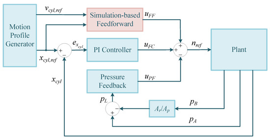
Figure 15.
Closed-loop control strategy with simulation-based feedforward.
By fusing simulated and measured signals at the control output stage (rather than merging raw sensor and simulation data), this approach leverages both real-time simulation and sensor feedback.
5. Implementation, Validation, and Experimental Results
This section presents the implementation of the simulation-based control system, model validation through parameter tuning and eigenfrequency matching, experimental testing, and final motion control tests.
5.1. Code Generation and Deployment
To enable simulation-based control, the real-time model must run on the IPC. Using the Simulink PLC Coder support package, it is possible to automatically generate Structured Text code directly from a Simulink subsystem. However, the Simulink model must be configured appropriately to ensure that the generated code accurately reflects the intended functionality.
First, all integrator, derivative, and transfer function blocks are replaced with their discrete-time equivalents by applying a zero-order hold approach, using MATLAB c2d to transform continuous parameters into discrete ones. The Simulink solver is then switched from a continuous solver to a discrete solver, with the fixed step size set to match the desired real-time controller cycle. This workflow enables users to design and fine-tune an intuitive Simulink model, featuring block diagrams and MATLAB functions, before automatically generating the more labor-intensive Structured Text code.
Figure 16 illustrates how the real-time model in the IPC compares to the corresponding model in Simulink. From a single Simulink subsystem, a single function block is generated in Structured Text. Consequently, the complexity of the Structured Text function block depends on how many functional blocks (e.g., integrators, custom functions) are contained within the Simulink subsystem. In the actual implementation, the integrator blocks use a forward Euler approach on the real-time controller.
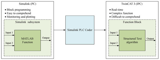
Figure 16.
Comparison between the model in Simulink and the model deployed on TwinCAT 3.
To streamline the deployment process, the hydraulic model and the mechanical model are created as two separate Simulink subsystems. When converting these subsystems to Structured Text, two separate function blocks are generated, one for the mechanical model and one for the hydraulic model. In TwinCAT 3, these function blocks are each called within their own program, which can then be assigned to specific logical processor cores on the real-time controller. This arrangement makes it possible to run the control system and sensor acquisition on one core while running the models on another.
For example, the simulation can operate at the lowest possible cycle time of to capture high-frequency dynamics, while the control loop often runs at a more practical interval of to . By separating the computation of the models from the control algorithm, the system can make more efficient use of the available processor resources while maintaining stable real-time performance.
5.2. Model Validation and Parameter Tuning
Model validation is an iterative tuning process that involves several factors. The model and the experimental setup (that is, the physical system) both receive the same input signal. The resulting outputs, specifically the piston position and the five hydraulic pressures, are then compared. If the simulated and measured quantities align sufficiently, the validation is deemed successful. Otherwise, the model is updated with new parameters, ensuring that any adjustments remain physically realistic. Throughout this process, continuous analysis of the system and the experimental results is crucial to understanding the underlying physics.
5.2.1. Parameter Tuning
Although many parameters affect system behavior, Table 4 lists the key parameters adjusted during tuning along with their final values.
Table 4.
Final values of key tuning parameters.
5.2.2. Eigenfrequency Matching and Error Analysis
An important aspect of the validation process is to verify that the eigenfrequency of the model aligns with that of the physical system. The eigenfrequency is fundamental to dynamic behavior, so it must be simulated accurately. This section presents both the procedure for measuring and adjusting the eigenfrequency of the mechanical system and an analysis of the observed discrepancies between the measured and simulated values.
In a mechanical assembly, multiple parameters affect the overall stiffness, including the material’s elasticity modulus (E), boundary conditions, and the geometry. In our model, E is used as an effective parameter that represents not only the stiffness of the crane arm but also the additional flexibility of the structural supports and bearings. By modifying E, the stiffness of the torsional spring connecting the lumped segments is adjusted, thus changing the overall stiffness and, consequently, the eigenfrequency of the system.
Due to the hydraulic cylinder constantly supporting the boom, isolating the boom’s dynamics is challenging. Therefore, eigenfrequency tests were performed with the load-holding valve closed, effectively decoupling the boom and cylinder dynamics from the remaining hydraulic components. An oscillation test was performed on both the physical system and the simulation:
- Physical system: the payload is manually lifted and released, initiating vibrations in the boom.
- Simulation model: the boom is initially held at rest and then allowed to drop slightly onto the cylinder under gravity.
Figure 17 illustrates the measurement of the eigenfrequency in both cases, calculated as
where n is the number of oscillation periods observed over the duration .
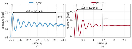
Figure 17.
Estimating the eigenfrequency of the boom and cylinder: (a) Measured data. (b) Simulation results.
The tests were performed at three different strokes of the cylinder ( = 100 mm, 200 mm, and 400 mm) to ensure robustness throughout the operating envelope. Table 5 compares the measured and simulated eigenfrequencies.
Table 5.
Comparison of measured and simulated eigenfrequencies for different cylinder strokes.
Error Analysis
It is well known from theoretical modeling that the eigenfrequency of a simulated system tends to be stiffer than that of the actual physical system. In our setup, the physical boom is mounted on a metal frame. The inherent flexibility of this frame, along with the slack in the attachment points, reduces the effective stiffness of the real assembly, factors not fully captured by the idealized theoretical model. Modeling these effects in full detail would significantly increase computational demands. Consequently, we adopted a practical approach by reducing the effective elasticity modulus E in our simulation, thus lowering the simulated eigenfrequency to better match experimental observations across various stroke lengths of the cylinder.
In addition to the eigenfrequency adjustment, an energy check was performed to verify proper energy conservation during oscillatory motion. Although the energy check confirmed that energy was conserved within acceptable limits, its detailed discussion was omitted for brevity since no significant discrepancies affecting dynamic behavior were observed.
Overall, the combination of eigenfrequency tuning and the accompanying error analysis gives us confidence that our simplified three-segment model captures the essential dynamic characteristics of the system despite the unavoidable simplifications.
5.2.3. Experimental Validation Results
The model was validated on two different velocity profiles, () and (). In the following, we focus on the results for the highest velocity set point, .
Figure 18, Figure 19, Figure 20, Figure 21, Figure 22 and Figure 23 compare the real-time simulation with experimental measurements for the position of the piston and four pressure signals at . Table 6 consolidates the peak and RMS errors, including eigenfrequency data for piston pressure.
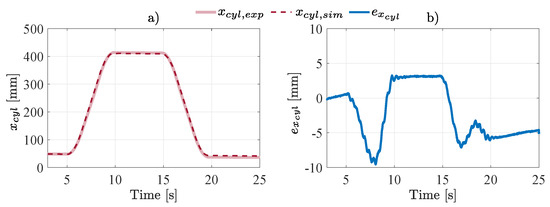
Figure 18.
Simulated piston position vs. experimental data: (a) Trapezoidal motion reference with . (b) Error between signals.
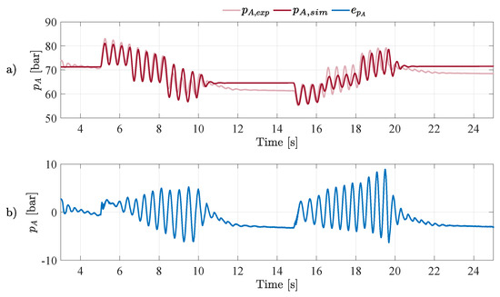
Figure 19.
Simulated vs. experimental piston pressure : (a) Pressure signals. (b) Error between signals.
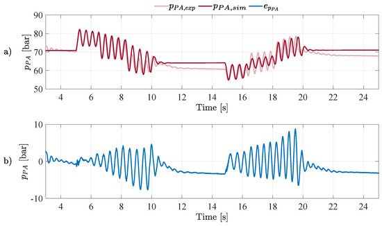
Figure 20.
Simulated vs. experimental pump-side pressure : (a) Pressure signals. (b) Error.
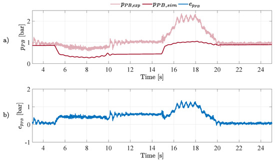
Figure 21.
Simulated vs. experimental pump-side pressure : (a) Pressure signals. (b) Error.
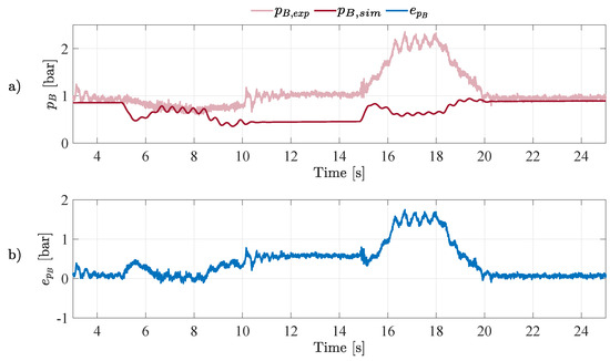
Figure 22.
Simulated vs. experimental rod pressure : (a) Pressure signals. (b) Error.
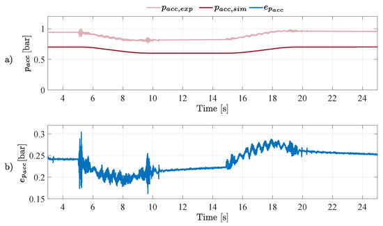
Figure 23.
Simulated vs. experimental accumulator pressure : (a) Pressure signals. (b) Error.
Table 6.
Peak and RMS error data at . Eigenfrequency values () appear for piston pressure.
5.3. Motion Control
Tests corresponding to typical working cycles are conducted to evaluate three different control strategies under two velocity set points, and . The velocity set points are tested to assess the system across a significant portion of the cylinder’s stroke range while avoiding mechanical end stops. The tests are based on the trapezoidal motion profile illustrated in Figure 24, where the trajectory of the piston of the cylinder starts at , extends to , and then retracts to the initial position. The ramp time is configured as , and the dwell time is set to .
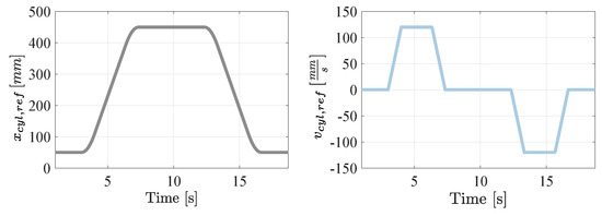
Figure 24.
Trapezoidal motion reference with .
5.3.1. Test 1: Open-Loop Benchmark Velocity Feedforward vs. Simulation-Based Feedforward
Figure 25 compares the piston position and tracking error for these two open-loop controllers at . The simulation-based feedforward yields a peak error of and an RMS error of . Meanwhile, the benchmark velocity feedforward has a peak error of and an RMS error of . Detailed results for both set points appear in Table 7.
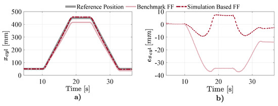
Figure 25.
Open-loop position tracking at : (a) Reference vs. measured piston position. (b) Tracking error.
Table 7.
Peak and RMS errors: benchmark velocity feedforward vs. simulation-based feedforward (open-loop).
5.3.2. Test 2: Open-Loop Simulation-Based Feedforward vs. Full Benchmark Controller
Figure 26 illustrates how the open-loop simulation-based feedforward compares to the closed-loop benchmark controller (including velocity feedforward, PI, and active damping). At , the closed-loop benchmark achieves an RMS error of , whereas the open-loop simulation-based feedforward yields . Table 8 lists the corresponding results at both velocities.
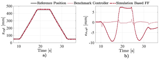
Figure 26.
Open-loop simulation-based feedforward vs. closed-loop benchmark at : (a) Piston positions. (b) Tracking error.
Table 8.
Peak and RMS errors: benchmark closed-loop controller vs. simulation-based feedforward (open-loop).
5.3.3. Test 3: Closed-Loop Benchmark Controller vs. Closed-Loop with Simulation-Based Feedforward
Lastly, the proposed simulation-based feedforward replaces the standard velocity feedforward within the same closed-loop structure (PI + active damping). Figure 27 shows the piston position at . As reported in Table 9, the benchmark system has an RMS error of , whereas the new closed-loop with simulation-based feedforward reduces it to .
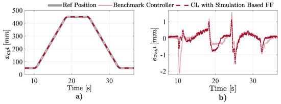
Figure 27.
Closed-loop control at : (a) Reference vs. measured piston position. (b) Tracking error.
Table 9.
Peak and RMS errors: benchmark closed-loop vs. closed-loop with simulation-based feedforward.
6. Discussion
This section discusses the main findings of the study with respect to system modeling, real-time simulation, and control design and outlines potential directions for future work.
6.1. Modeling and Real-Time Simulation
A key achievement of this work is the real-time deployment of a nonlinear high-fidelity model on an IPC. Comparisons between the Simulink model and the Structured Text implementation in TwinCAT show minimal numerical integration discrepancies. Specifically, no linearization was required, which broadens the feasibility of real-time simulation for complex nonlinear systems. Furthermore, the tight correspondence between the real-time model and Simulink enables comprehensive parameter tuning in Simulink, followed by rapid code generation via the Simulink PLC Coder.
To ensure real-time performance, certain modeling assumptions were introduced. For example, the flexible crane boom was represented as a planar mechanism, and moment equilibrium equations were formulated in terms of relative angles rather than Cartesian coordinates. This approach successfully captured the dynamic behavior while limiting computational overhead.
The final validation yielded an RMS pressure error below for the main cylinder pressures ( and ) and achieved an eigenfrequency accuracy of approximately 97%. The tuning process addressed piston position, hydraulic pressures, and eigenfrequencies across various cylinder strokes. Discrepancies persisted primarily in low-speed scenarios, where friction modeling was less accurate—specifically, the assumption of zero-velocity friction does not reflect the non-zero friction of the real system near rest. Incorporating a more advanced friction model (e.g., LuGre) may mitigate this limitation, though it would increase computational costs.
Furthermore, the tuning process highlighted the importance of fluid compression in explaining the measured position and pressure responses, particularly at lower velocities. Dissolved air significantly affects the bulk modulus of the fluid, and initial leakage-only models were insufficient to capture these effects. By incorporating variable bulk modulus physics, the model accurately represented the transition between low and high pressures under moderate operating conditions.
Regarding the flexible boom, the eigenfrequency analysis revealed that the model initially overestimated the stiffness of the system. In practice, the boom is mounted on a metal frame, and the inherent flexibility of the frame, along with the slack at the attachment points, reduces the effective stiffness of the physical system. Detailed modeling of these effects would be computationally intensive; therefore, the effective modulus of elasticity E was reduced, bringing the simulated eigenfrequency closer to alignment with the experimental measurements at various stroke lengths of the cylinder. An energy check was also performed to confirm energy conservation during oscillatory motion, but its detailed discussion was omitted for the sake of brevity, as it did not reveal any significant discrepancies.
6.2. Simulation-Based Control
Two principal control strategies were tested: a pure open-loop feedforward and a closed-loop controller that integrates simulation-based feedforward with sensor feedback. Under open-loop conditions, the simulation-based feedforward significantly outperformed the benchmark model-based velocity feedforward, reducing the RMS tracking error by up to 83%. This improvement was most pronounced at lower velocities, where unmodeled leakage and compressibility effects accumulate; the more accurate real-time simulation helped account for these factors.
In contrast, the benchmark closed-loop controller delivered higher accuracy (for example, an RMS error of versus ), reflecting the advantage of sensor feedback in managing unmodeled disturbances. Although the simulation’s own RMS error in the piston position was approximately at higher speeds, indicating that submillimeter open-loop tracking remains challenging, the integration of simulation-based feedback into the closed-loop system reduced the RMS error by approximately 12% at higher speeds and 16% at lower speeds, particularly during transient load lifting phases. Given that the benchmark system already achieves errors below at slower speeds, the magnitude of improvement depends on the precision requirements of the application.
6.3. Further Work
Future research will focus on refining friction and fluid compressibility models, especially under near-zero velocity conditions and partial-load operation. More advanced friction models, such as LuGre or physics-informed machine learning approaches, could address residual discrepancies, albeit at increased computational cost. In addition, extended Kalman filtering or complementary filtering methods might be employed to merge measured states with simulated estimates, leveraging the predictive capabilities of the model alongside sensor feedback.
Another avenue for future research is to perform a comprehensive sensitivity analysis. Although our current work discusses how variations in key parameters affect the simulation, we have not explored in detail how these variations influence control performance. Such an analysis would help to understand the robustness of the control system and optimize parameter tuning for improved control accuracy.
Furthermore, we plan to extend our experimental evaluation to more complex test setups that include multiple degrees of freedom as well as varying load conditions and motion directions. By testing the proposed controller under scenarios involving multidirectional motion, frequent start–stop events, and variable loads, we aim to more closely simulate the practical industrial conditions that a manipulator may face.
Finally, we plan to extend our approach towards developing a digital twin of the electro-hydraulic system for enhanced predictive maintenance. The real-time simulation model, which accurately captures multi-domain dynamics, can serve as a virtual replica of the physical system. By fusing real-time sensor data with the simulation, deviations from expected performance can be detected promptly, enabling early fault detection and proactive maintenance scheduling. This integration will provide a powerful tool to improve system reliability and reduce downtime in industrial applications.
7. Conclusions
A real-time, nonlinear model of the electro-hydraulic actuator and flexible boom was successfully implemented on an industrial PC. Reducing the boom to three lumped segments provided a balance between computational speed and fidelity, allowing precise replication of the dynamic behavior of the physical system. Hydraulic and mechanical models were implemented as separate Simulink subsystems, allowing efficient deployment as function blocks in TwinCAT 3. This arrangement enabled the control system and sensor acquisition to run on one processor core while the models executed on another, optimizing processor resources and ensuring stable real-time performance. The simulation operated at a cycle time of to capture high-frequency dynamics, while the control loop ran at an interval of .
Through iterative tuning of the model parameters, the following key outcomes were achieved:
- Objective 1 (model fidelity): a piston position RMS error below (1.2% of the overall stroke length) and an accuracy of the eigenfrequency of approximately 97%.
- Objective 2 (control improvement): an 83% reduction in the RMS tracking error relative to the benchmark model-based velocity feedforward and a 16% improvement in closed-loop position tracking when combining simulation-based feedforward with the benchmark controller.
Although these results confirm that the real-time model cannot fully replace sensor feedback for high-precision tracking, they also demonstrate that simulation-based feedforward can significantly outperform simpler open-loop methods. In addition, when integrated into a closed-loop scheme, the model further enhances control accuracy. Furthermore, high-fidelity simulation provides a strong foundation for future work in predictive maintenance and digital twin development. By fusing real-time sensor data with simulation, future systems could enable early fault detection, optimized maintenance scheduling, and improved overall system reliability. In line with this, we plan to extend our experimental evaluation to include test setups with additional degrees of freedom and conditions featuring variable loads and changing motion directions. These extensions will help assess the performance of the proposed controller in more complex and realistic scenarios, further demonstrating the applicability of our approach to practical industrial applications.
Author Contributions
Conceptualization, D.H., K.A.H. and J.H.; methodology, D.H., K.A.H. and J.H.; software, K.A.H. and J.H.; validation, K.A.H. and J.H.; formal analysis, K.A.H. and J.H.; investigation, K.A.H. and J.H.; resources, K.A.H., J.H. and D.H.; data curation, K.A.H. and J.H.; writing—original draft preparation, K.A.H., J.H. and D.H.; writing—review and editing, D.H., K.A.H., J.H. and M.R.H.; visualization, K.A.H., J.H. and D.H.; supervision, D.H. and M.R.H.; project administration, D.H.; funding acquisition, D.H. All authors have read and agreed to the published version of the manuscript.
Funding
This research was funded by the Mechatronics Section, Department of Engineering Sciences, University of Agder.
Informed Consent Statement
Not applicable.
Data Availability Statement
The data supporting this study are available upon request. Please contact the corresponding author for access.
Acknowledgments
The work presented in this paper is based on the results obtained in an unpublished MSc thesis in Mechatronics entitled “Simulation-Based Control of an Electro-Hydraulic Actuated Flexible Boom”, conducted at the University of Agder during the spring of 2024 by Kathrine Als Hansen and Jonas Holmen, supervised by Daniel Hagen and Mohammad Poursina.
Conflicts of Interest
The authors declare no conflicts of interest.
Correction Statement
This article has been republished with a minor correction to resolve spelling and grammatical errors, including Section 3.2 and Section 3.2.1, Figure 10, Equations (18), (25) and (27), Acknowledgments section and Appendix B. These changes do not affect the scientific content of the article.
Abbreviations
The following abbreviations are used in this manuscript:
| IPC | Industrial PC |
| PID | Proportional–Integral–Derivative |
| SCC | Self-Contained Electro-Hydraulic Cylinder |
| DCV | Directional Control Valve |
| APM | Axial Piston Machine |
| SM | Servo Motor |
| POCV | Pilot-Operated Check Valve |
| PLC | Programmable Logic Controller |
| CPU | Central Processing Unit |
| FF | FeedForward |
| FBD | Free Body Diagram |
| KD | Kinetic Diagram |
Appendix A. Electro-Hydraulic Actuation System
Appendix A.1. Valve Flow Equations
Internal leakage is expressed as
where is the leakage constant and is the pressure difference.
The drain flows of the case are modeled as follows. For side A:
where is the valve constant, and is the pressure difference.
For side B:
where is the valve constant, and is the pressure difference.
The flow through check valves is determined using the dimensionless opening:
where is the crack pressure and is the full open pressure.
The valve constant is computed as
where , is the nominal flow, and is the nominal pressure.
The effective valve constant for valves in series is
where are the valve constants.
Specific path flows are described as follows: For :
where is the effective valve constant.
For :
where is the valve constant.
For :
where is the effective valve constant.
Cylinder flows are as follows:
where is the valve constant for ,
where is the valve constant for .
Appendix A.2. Pressure Dynamics
Appendix A.2.1. Cylinder
The pressure gradients for the high-pressure side () and the low-pressure side () of the cylinder are:
where and represent the effective stiffness values of the oil, while and correspond to the piston area and the rod side ring (annulus) area, respectively (see Figure 6). and are the initial oil volumes, and denotes the piston velocity.
Appendix A.2.2. Accumulator
The accumulator acts as a hydraulic reservoir, storing and releasing fluid as required by the system. Figure A1 illustrates the bladder accumulator used in the system.

Figure A1.
Bladder Accumulator.
Figure A1.
Bladder Accumulator.

The pressure in the gas and liquid chambers, , is always equal due to force equilibrium. The total accumulator volume, , consists of the gas volume () and the fluid volume (), expressed as
where the gas obeys the polytropic gas law:
and is the polytropic index. The value of depends on the type of process: for an adiabatic process (when ) and for an isothermal process (when ).
Initially, the accumulator is preloaded with a pressure, , which is the lowest allowable value to avoid exceeding the pressure capacity of the suction line on side B of the pump. The initial gas volume, , can be calculated using the preloaded pressure and volume:
where is the initial preloaded volume. The preloaded pressure is set during manufacturing to pressurize the gas in the accumulator, while the initial pressure is determined under working conditions after the system is filled with hydraulic fluid.
The dynamic behavior of the accumulator is governed by the time derivatives of the governing equations. Differentiating the total volume equation (Equation (A14)) yields the relationship between the volume gradients of the gas and fluid:
which indicates that any increase in fluid volume results in an equal decrease in gas volume, and vice versa.
Differentiating the gas law (Equation (A15)) using the product rule yields:
Rearranging and solving for gives:
Substituting Equation (A19) into the general pressure gradient equation, the final expression for the pressure gradient is derived:
The net flow into the accumulator accounts for all system interactions and is given by:
where and are the drain flows in the case, is the output flow, and and are the flows of the specific system.
Appendix B. Flexible Boom Mechanism
Appendix B.1. Dynamic Analysis for Body 3
Since the system consists of three interconnected bodies, three equations of motion are derived. These are based on three sets of diagrams: one for body 3 (Figure A2), one for the combined bodies 2 and 3 (Figure A3), and one for the entire system comprising all three bodies (Figure 11).
As illustrated in Figure A2, the key components in the analysis are: , the torsional damper torque; , the torsional spring torque; , the gravitational force acting on body 3; , the mass of body 3; , the acceleration of the center of mass of body 3; , the moment of inertia around the center of mass of body 3; , the angular acceleration of body 3; and and , the reaction forces at point C.

Figure A2.
Free body diagram (left) and kinetic diagram (right) for body 3.
Figure A2.
Free body diagram (left) and kinetic diagram (right) for body 3.

From the free body diagram and the kinetic diagram in Figure A2, the equation of moments about point C is derived as
where the hat vector is defined as
Since the moment is taken about the point C, the reaction forces and do not contribute to the moment. This simplifies the analysis by eliminating terms that would otherwise complicate the calculation.
Here, the linear acceleration of body 3’s mass center, , is divided into two components: (1) terms related to the angular accelerations of the segments and (2) terms dependent on squared angular velocities. The latter are grouped into the vector .
The vector , which contains terms unrelated to angular accelerations, is given by:
Reorganizing the terms, the moment equation becomes:
Finally, Equation (A25) is generalized and expressed in matrix form:
where represents the applied moments on the left-hand side, while the coefficient matrix and the angular acceleration vector are on the right-hand side.
Appendix B.2. Dynamic Analysis for Bodies 2 and 3
Using the same method, the terms in Equation (A28) are derived for all three bodies. Figure A3 illustrates the analysis for bodies 2 and 3, from which the corresponding equations are retrieved.

Figure A3.
Free body diagram and kinetic diagram of two lumped segments.
Figure A3.
Free body diagram and kinetic diagram of two lumped segments.

The equation of moments for the combined system of bodies 2 and 3 about point B is expressed as
where and represent the torsional spring and damping torques acting between body 1 and body 2. The gravitational forces acting on bodies 2 and 3 are denoted by and , while the angular accelerations are and .
References
- Dwivedy, S.K.; Eberhard, P. Dynamic analysis of flexible manipulators, a literature review. Mech. Mach. Theory 2006, 41, 749–777. [Google Scholar] [CrossRef]
- Subedi, D.; Tyapin, I.; Hovland, G. Modeling and analysis of flexible bodies using lumped parameter method. In Proceedings of the 2020 IEEE 11th International Conference on Mechanical and Intelligent Manufacturing Technologies (ICMIMT), Cape Town, South Africa, 20–22 January 2020; pp. 161–166. [Google Scholar] [CrossRef]
- Mamo, M.B.; Ebbesen, M.K.; Poursina, M. Dynamic Modelling and Simulation of Two-link Flexible Robot Using Rayleigh Beam Theory. In Proceedings of the 2023 11th International Conference on Control, Mechatronics and Automation (ICCMA), Grimstad, Norway, 1–3 November 2023; pp. 164–169. [Google Scholar] [CrossRef]
- Subudhi, B.; Morris, A. Dynamic modelling, simulation and control of a manipulator with flexible links and joints. Robot. Auton. Syst. 2002, 41, 257–270. [Google Scholar] [CrossRef]
- Orošnjak, M.; Jocanović, M.; Karanović, V. Simulation and modeling of a hydraulic system in FluidSim. In Proceedings of the XVII International Scientific Conference on Industrial Systems (IS’17), Novi Sad, Serbia, 4–6 October 2017; p. 4. [Google Scholar]
- Zhang, P.; Hu, W.; Cao, W.; Chen, L.; Wu, M. Multi-fault diagnosis and fault degree identification in hydraulic systems based on fully convolutional networks and deep feature fusion. Neural Comput. Appl. 2024, 36, 9125–9140. [Google Scholar] [CrossRef]
- Dai, J.; Tang, J.; Huang, S.; Wang, Y. Signal-Based Intelligent Hydraulic Fault Diagnosis Methods: Review and Prospects. Chin. J. Mech. Eng. 2019, 32, 75. [Google Scholar] [CrossRef]
- Nguyen, D.; Huynh, V.K.; Robbersmyr, K.G. Training Scheme for Convolutional Neural Network Based Multiple Fault Classifier of Permanent Magnet Synchronous Motors Under Variable Speed and Load Conditions. In Proceedings of the 2024 International Conference on Electrical Machines (ICEM), Torino, Italia, 1–4 September 2024; pp. 1–7. [Google Scholar] [CrossRef]
- Kandukuri, S.T.; Senanyaka, J.S.L.; Huynh, V.K.; Robbersmyr, K.G. A Two-Stage Fault Detection and Classification Scheme for Electrical Pitch Drives in Offshore Wind Farms Using Support Vector Machine. IEEE Trans. Ind. Appl. 2019, 55, 5109–5118. [Google Scholar] [CrossRef]
- Lal Senanayaka, J.S.; Van Khang, H.; Robbersmvr, K.G. CNN based Gearbox Fault Diagnosis and Interpretation of Learning Features. In Proceedings of the 2021 IEEE 30th International Symposium on Industrial Electronics (ISIE), Kyoto, Japan, 20–23 June 2021; pp. 1–6. [Google Scholar] [CrossRef]
- Zhang, Y.; Ding, W.; Deng, H. Reduced Dynamic Modeling for Heavy-Duty Hydraulic Manipulators with Multi-Closed-Loop Mechanisms. IEEE Access 2020, 8, 101708–101720. [Google Scholar] [CrossRef]
- Kim, M.; Lee, S.U.; Kim, S.S. Real-Time Simulator of a Six Degree-of-Freedom Hydraulic Manipulator for Pipe-Cutting Applications. IEEE Access 2021, 9, 153371–153381. [Google Scholar] [CrossRef]
- Huston, R.L.; Wang, Y. Flexibility Effects in Multibody Systems. In Computer-Aided Analysis of Rigid and Flexible Mechanical Systems; Seabra Pereira, M.F.O., Ambrósio, J.A.C., Eds.; Springer: Dordrecht, The Netherlands, 1994; pp. 351–376. [Google Scholar] [CrossRef]
- Franklin, G.F.; Powell, J.D.; Emami-Naeini, A.; Powell, J.D. Feedback Control of Dynamic Systems; Prentice Hall: Upper Saddle River, NJ, USA, 2002. [Google Scholar]
- Zhang, Q. Hydraulic linear actuator velocity control using a feedforward-plus-PID control. Int. J. Flex. Autom. Integr. Manuf. 1999, 7, 277–292. [Google Scholar]
- Jensen, K.J.; Ebbesen, M.K.; Hansen, M.R. Online Deflection Compensation of a Flexible Hydraulic Loader Crane Using Neural Networks and Pressure Feedback. Robotics 2022, 11, 34. [Google Scholar] [CrossRef]
- Finkeldey, F.; Saadallah, A.; Wiederkehr, P.; Morik, K. Real-time prediction of process forces in milling operations using synchronized data fusion of simulation and sensor data. Eng. Appl. Artif. Intell. 2020, 94, 103753. [Google Scholar] [CrossRef]
- Saadallah, A.; Finkeldey, F.; Buß, J.; Morik, K.; Wiederkehr, P.; Rhode, W. Simulation and sensor data fusion for machine learning application. Adv. Eng. Inform. 2022, 52, 101600. [Google Scholar] [CrossRef]
- Padovani, D.; Ketelsen, S.; Hagen, D.; Schmidt, L. A Self-Contained Electro-Hydraulic Cylinder with Passive Load-Holding Capability. Energies 2019, 12, 292. [Google Scholar] [CrossRef]
- Hagen, D.; Padovani, D.; Choux, M. A Comparison Study of a Novel Self-Contained Electro-Hydraulic Cylinder versus a Conventional Valve-Controlled Actuator—Part 1: Motion Control. Actuators 2019, 8, 79. [Google Scholar] [CrossRef]
- Sørensen, J.K.; Hansen, M.R.; Ebbesen, M.K. Numerical and Experimental Study of a Novel Concept for Hydraulically Controlled Negative Loads. Model. Identif. Control. 2016, 37, 195–211. [Google Scholar] [CrossRef]
- Hagen, D.; Padovani, D.; Choux, M. Design and Implementation of Pressure Feedback for Load-Carrying Applications with Position Control. In Proceedings of the Sixteenth Scandinavian International Conference on Fluid Power, Tampere, Finland, 22–24 May 2019; pp. 22–24. [Google Scholar]


Disclaimer/Publisher’s Note: The statements, opinions and data contained in all publications are solely those of the individual author(s) and contributor(s) and not of MDPI and/or the editor(s). MDPI and/or the editor(s) disclaim responsibility for any injury to people or property resulting from any ideas, methods, instructions or products referred to in the content. |
© 2025 by the authors. Licensee MDPI, Basel, Switzerland. This article is an open access article distributed under the terms and conditions of the Creative Commons Attribution (CC BY) license (https://creativecommons.org/licenses/by/4.0/).