Abstract
The X-ray defect detection system for weld seams in deep-sea manned spherical shells is nonlinear and complex, posing challenges such as motor parameter variations, external disturbances, coupling effects, and high-precision dual-motor coordination requirements. To address these challenges, this study proposes a deep reinforcement learning-based control scheme, leveraging DRL’s capabilities to optimize system performance. Specifically, the TD3 algorithm, featuring a dual-critic structure, is employed to enhance control precision within predefined state and action spaces. A composite reward mechanism is introduced to mitigate potential motor instability, while CP-MPA is utilized to optimize the performance of the proposed m-TD3 composite controller. Additionally, a synchronous collaborative motion compensator is developed to improve coordination accuracy between the dual motors. For practical implementation and validation, a PMSM simulation model is constructed in MATLAB/Simulink, serving as an interactive training platform for the DRL agent and facilitating efficient, robust training. The simulation results validate the effectiveness and superiority of the proposed optimization strategy, demonstrating its applicability and potential for precise and robust control in complex nonlinear defect detection systems.
1. Introduction
Since the 20th century, deep-sea environments have attracted extensive exploration due to their abundant natural resources and high scientific value. Ensuring the structural integrity of manned deep-sea vehicles in such harsh conditions is critical. In our previous research, we developed an X-ray defect detection system for weld seams in manned spherical shells. By integrating defect detection with three-dimensional reconstruction, we established a static-strength mechanical model for long-term service, enabling the effective detection and precise localization of weld defects. Prior to the initiation of each deep-sea exploration mission, the inspection system conducts an independent defect assessment protocol on manned pressure hulls that have completed extended service durations, thereby ensuring the preservation of their structural integrity. During this critical evaluation phase, the manned pressure hull undergoes detachment from the submersible vehicle and subsequent placement within a controlled testing environment specifically engineered for comprehensive defect detection operations. This paper focuses on an optimization method for the motion control of defect detection systems.
Control of the drive motor is crucial for the performance of the defect detection system. However, the motor’s complex time-varying nonlinear characteristics and the requirement for precise control in defect detection pose significant challenges to the system. PMSMs have attracted the attention of industry and academia due to their advantages in control theory and structural adaptability, and have developed rapidly in the past few decades [1]. In the early application of the PMSM, a control strategy based on AC stator voltage and open-loop control was applied [2,3]. In the 1980s, the introduction of vector control theory represented by DTC and FOC greatly improved motor control methods [4,5]. FOC decomposes the stator current to control the torque through the magnetic field, while the DTC simplification theory directly performs sensorless flux control [6].
Although the PID controller is renowned for its simplicity and ease of implementation, it struggles to address complex and severe control challenges [7]. In the 1950s, V. I. Utkin advanced sliding mode control theory by establishing a sliding surface and dynamically adapting control strategies [8]. With the development of control theory, fuzzy control has been applied. Complete fuzzy control includes fuzzification, a rule base, an inference mechanism, and a defuzzification process, which has great advantages in dealing with time-varying complex uncertain systems [9,10,11]. In addition, controller optimization based on a swarm intelligence optimization algorithm is also an important research direction. N. F. Mohammed et al. improved the performance of the PID controller by introducing genetic algorithm (GA) tuning [12], while Zwe-Lee Gaing et al. applied particle swarm optimization (PSO) to controller optimization [13]. In addition, various swarm intelligence algorithms, including the Grey Wolf Optimizer (GWO), Slime Mould Algorithm (SMA), and Marine Predator Algorithm (MPA), have demonstrated effectiveness in the field of control. Swarm intelligence optimization remains a research hotspot in control systems.
In recent years, neural network-based control schemes have demonstrated significant advantages, particularly in nonlinear disturbance environments. Previous studies have validated the effectiveness of torque and speed control for asynchronous motors utilizing neural network-based feedforward and feedback architectures [14]. Artificial neural networks usually require a large amount of labeled data during the training process. In industrial applications, the accuracy and efficiency of machine learning-based flexible rectifier state prediction models have been empirically validated [15]. Moreover, deep learning LSTM networks have been employed in sensor response prediction studies to characterize the mapping between electrical resistance and tensile strain [16]. It is evident that these supervised learning approaches require substantial data support—a prerequisite that is often challenging to fulfill in practical engineering applications. In contrast, reinforcement learning optimizes control policies through interaction with the environment, making it more suitable for engineering practice. Early reinforcement learning combined Monte Carlo and temporal difference methods to address system modeling uncertainties [17]. In 2013, Volodymyr Mnih and DeepMind proposed integrating deep neural networks into RL, introducing the end-to-end learning-based DQN algorithm and marking the beginning of deep reinforcement learning [18]. Subsequently, deep reinforcement learning has attracted extensive research interest, leading to numerous advanced algorithms such as A3C [19], DDPG [20], PPO [21], TD3 [22], and SAC [23]. Shuprajhaa et al. proposed adaptive controllers combined with deep reinforcement learning, developing a data-driven improved PPO method [24]. Dogru et al. introduced offline training followed by online fine-tuning, effectively enhancing training efficiency and mitigating losses in industrial applications [25]. Additionally, Bloor et al. proposed a CIRL framework to integrate prior knowledge into deep reinforcement learning agents [26].
This paper proposes a deep reinforcement learning-based control optimization method for defect detection systems. CP-MPA is enhanced via chaotic map initialization and an improved population mechanism to form the m-TD3 composite controller, thereby enabling adaptive control. The TD3 agent architecture is tailored to improve stability in complex, unstable environments and expedite training. Moreover, a synchronous cooperative motion compensator based on cross-coupling control [27] is developed to further refine detection accuracy. Comparative simulations against traditional PID, MPA-optimized PID, and standalone TD3 controllers validate the efficacy of the proposed approach, underscoring its potential for industrial applications.
2. Design and Control Principles of the Defect Detection System
2.1. X-Ray Defect Detection System for Deep-Sea Manned Spherical Shell Welds
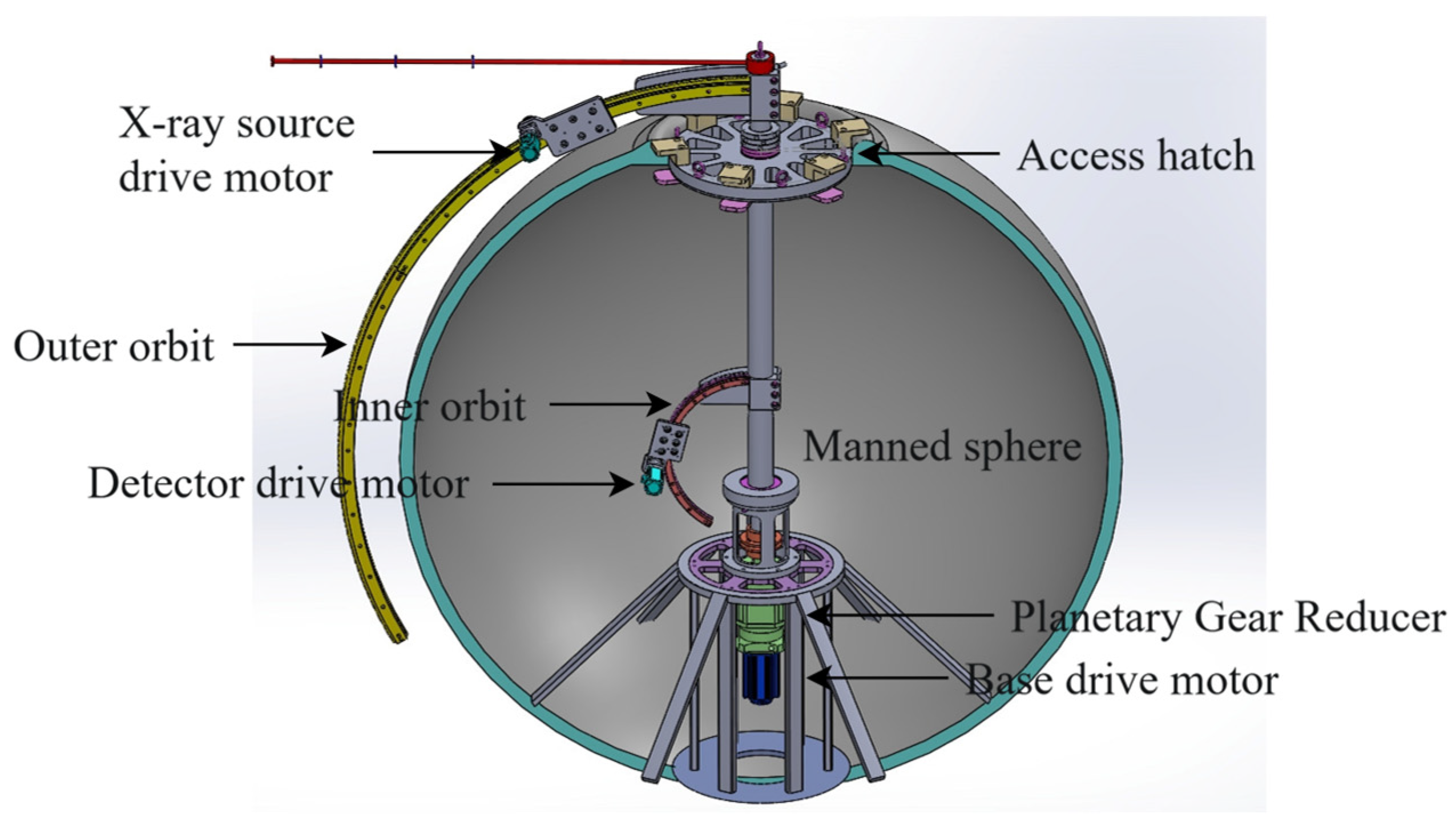
The spherical shell weld seam defect detection system architecture is structured around three core components: a CNT-based distributed cold-cathode X-ray inspection setup, a multi-actuator control mechanism for the detection process, and a data-driven method for identifying and recognizing defect information within image data.
The detection system employs an X-ray-based approach that integrates a carbon nanotube (CNT) array distributed X-ray source with a flat-panel detector to acquire multi-angle data from spherical shell welds. Its novelty lies in combining a cold-cathode X-ray source for conformal inspection with comprehensive 3D reconstruction. Within each CNT array tube, multiple emitters generate focal-spot exposures, while an internal architecture—comprising cathode, anode, gate, and focusing electrodes—enables a systematic, signal-controlled cathode layout that enhances source activation and exposure performance. In operation, the X-ray source captures images from various angles, and the detector, by registering transmitted X-rays, supplies data for subsequent 3D reconstruction. Exploiting sensitivity to X-ray-induced charge variations, the detector quantifies intensity based on the magnitude of charge change; for homogeneous metals, this intensity correlates with the traversed volume. Furthermore, the current generated in the selenium layer is stored in thin-film transistors, ensuring precise current-to-pixel alignment and enabling accurate, position-specific X-ray detection.
To achieve the complete 3D reconstruction and defect detection of the manned spherical shell, it is essential to obtain multi-perspective X-ray exposures of the entire structure. As shown in Figure 1, the system utilizes an integrated actuator drive mechanism based on permanent magnet synchronous motors. Coordinating three actuators—corresponding to the drive motors for the X-ray source, detector, and base—the system can scan the shell via independent or coordinated movements across three degrees of freedom. Concurrently, the control system modulates cathode signals to selectively activate multiple CNT-based distributed X-ray sources, capturing a greater number of angular exposures and detailed viewpoint-specific data once the relative positions of the source and detector are established. Both multi-actuator control and data communication are managed by an embedded controller, ensuring comprehensive system-level integration.

Figure 1.
Framework of deep-sea manned sphere shell weld X-ray defect detection system.
Data-driven defect detection is essential. In the spherical shell weld inspection system, defect features are extracted via object detection and semantic segmentation, and 3D reconstruction maps the shell and defects. High computational demands necessitate the offloading of X-ray image processing—including preprocessing, enhancement, reconstruction, and analysis—to an upper-level computer for comprehensive flaw identification.
The integration of actuator control is challenged by the reconciliation of detection resolution, detector dimensions, scanning angles, and magnification. Sub-100 µm defect detection is constrained by magnification-induced truncation, yielding clear reconstructions only within limited regions and depths while causing ghosting elsewhere. Moreover, the small scan coverage (~100 mm) relative to the 2100 mm shell necessitates multiple repositionings, where even minor misalignments disrupt the strict angular precision required. Thus, precise actuator control is essential for mitigating cumulative errors and ensuring accurate 3D reconstructions.
The defect detection system applies the m-TD3 algorithm to optimize actuator control and incorporates a synchronous collaborative compensator to mitigate coordination errors during multi-actuator cooperative motion, thereby providing precise scanning and positioning for the CNT-based distributed X-ray source and detector. This ensures that the system obtains X-ray images with accurately defined exposure angles, laying the groundwork for efficient three-dimensional reconstruction and defect recognition, and ultimately achieving high-resolution conformal inspection. The detection system has a diameter exceeding 3.3 m, has a maximum voltage of 120 kV, has a peak current of 75 μA, and is expected to attain a resolution notably better than 50 μm in the x-y plane and better than 150 μm in the z direction. A digital interpretation approach is established to correlate defect information with structural safety, and, by integrating deep learning-based defect detection, the system can efficiently identify various defects in manned spherical shells under long-term operational conditions.
2.2. Drive Motor Control Principle
The defect detection system utilizes permanent magnet synchronous motors (PMSMs) as drive units. The outer-track motor powers the distributed cold-cathode X-ray source, the inner-track motor propels the detector, and the central-axis motor facilitates the circumferential motion of both the inner and outer tracks. The coordinated control of these motors ensures sequential exposure across the entire spherical shell. Consequently, the overall detection performance is highly dependent on the precision of motor control.
The above equation represents the three-phase voltage equations of a PMSM, where denotes the three-phase voltage, is the stator resistance, represents the three-phase current, is the self-inductance of the three-phase windings, is the mutual inductance of the three-phase windings, denotes the permanent magnet flux linkage, and is the phase angle.
In order to simplify the motor model, the natural coordinate system is generally converted into the stationary coordinate system through Clark transformation, and on this basis, Park transformation is carried out and converted into the synchronous rotating coordinate system , and the voltage equation under the coordinate is obtained [28]:
The number of magnetic poles is , and the electromagnetic torque in the coordinates is [29]
The equation of mechanical motion is [29]
where is the moment of inertia, is the load torque, is the damping coefficient, and is the mechanical angular velocity [28].
It can be seen that the mechanical motion of the motor can be completely controlled by and . In order to improve the control effect, the feedforward compensation decoupling voltage equation needs to be added. The feedforward compensation formula is as follows:
With the application of the control simplified control theory, the -axis current-loop PI controller proportional gain is , the integral gain is , and the current-loop input control signal is ; then,
The closed-loop transfer function of the -axis current loop is as follows:
The speed-loop PI controller proportional gain is , the integral gain is , and the torque constant ; then,
The closed-loop transfer function of the speed loop is as follows:
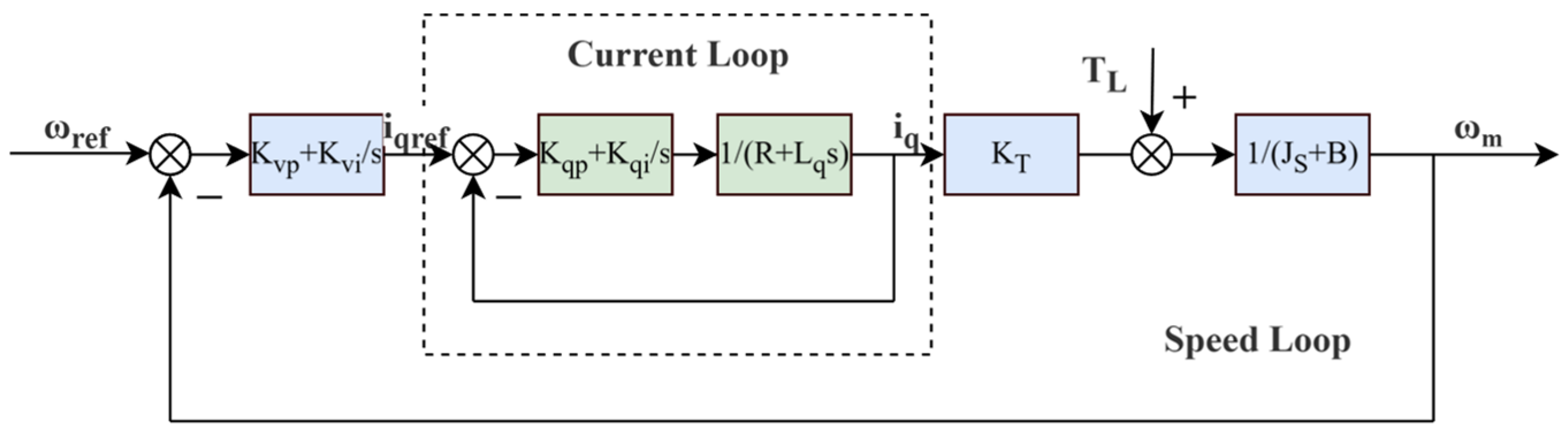
The theoretical control block diagram of the permanent magnet synchronous motor is shown in Figure 2. Based on this, a PMSM simulation model is built in the Simulink environment by applying the fundamental principles of electromagnetism, dynamics, and control theory. This model generates interaction data for the reinforcement learning agent. In addition, an approximate transfer function can be derived from the motor parameters and the closed-loop speed control transfer formula, providing a simplified model for experimental validation.
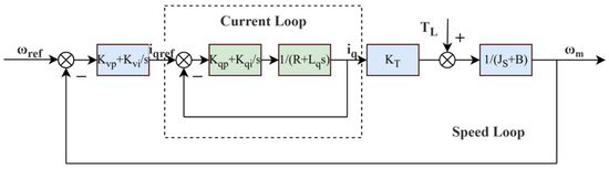
Figure 2.
Permanent magnet synchronous motor speed-loop control block diagram.
3. Control Optimization Based on Reinforcement Learning
The actuator control system proposed in this study is based on deep reinforcement learning (DRL). Unlike traditional control methods, which depend on explicit system models, DRL exhibits superior adaptability in managing nonlinear, complex systems with unknown dynamics. Its self-adaptive strategies are iteratively refined through training, enhancing responsiveness to dynamic scenarios and improving generalization. Furthermore, DRL’s advanced feature-extraction capabilities enable the mapping of intricate nonlinear relationships, thereby reducing reliance on manual design. Finally, its proficiency in processing high-dimensional continuous data further underpins its capacity to execute complex control tasks.
3.1. TD3 Algorithm
Scott Fujimoto et al. improved the DDPG algorithm and proposed the TD3 algorithm to solve the problem wherein excessive deviation in value estimation leads to an unsatisfactory strategy [22].
The TD3 algorithm initializes the main network and target network of the actor network and dual-critic network, conforming to the slow migration formula:
where is the mobility, is the weight of the target network, and is the main weight of the network. The target network migration strategy endows the algorithm with stability. In the RL interaction process, the actor network outputs action according to the current state , attains an environmental reward and the next state , and obtains a set of data and stores it in the experience pool. TD3 agents periodically batch randomly sampled data from the experience pool, avoiding highly correlated and similar training data while reducing extreme individual influence.
The training process is based on the action-value function and follows the Bellman expectation equation, which takes into account both and the expected cumulative reward of the policy guidance. The formula is [22]
where, represents how serious the critic network is about the future rewards of the strategy, and are the two target critic networks, and and are the weights of the main critic network and the target network. The double Q network combines the loss function and the gradient descent algorithm to update the network parameters, while the goal of the actor network is to maximize the reward; the gradient ascent method is used to update the weights, and the actor network update formula is [22]
where represents the output of the actor network in state , and is the weight of the actor network.
3.2. m-TD3 Composite Controller Based on Reinforcement Learning
3.2.1. Agent Design
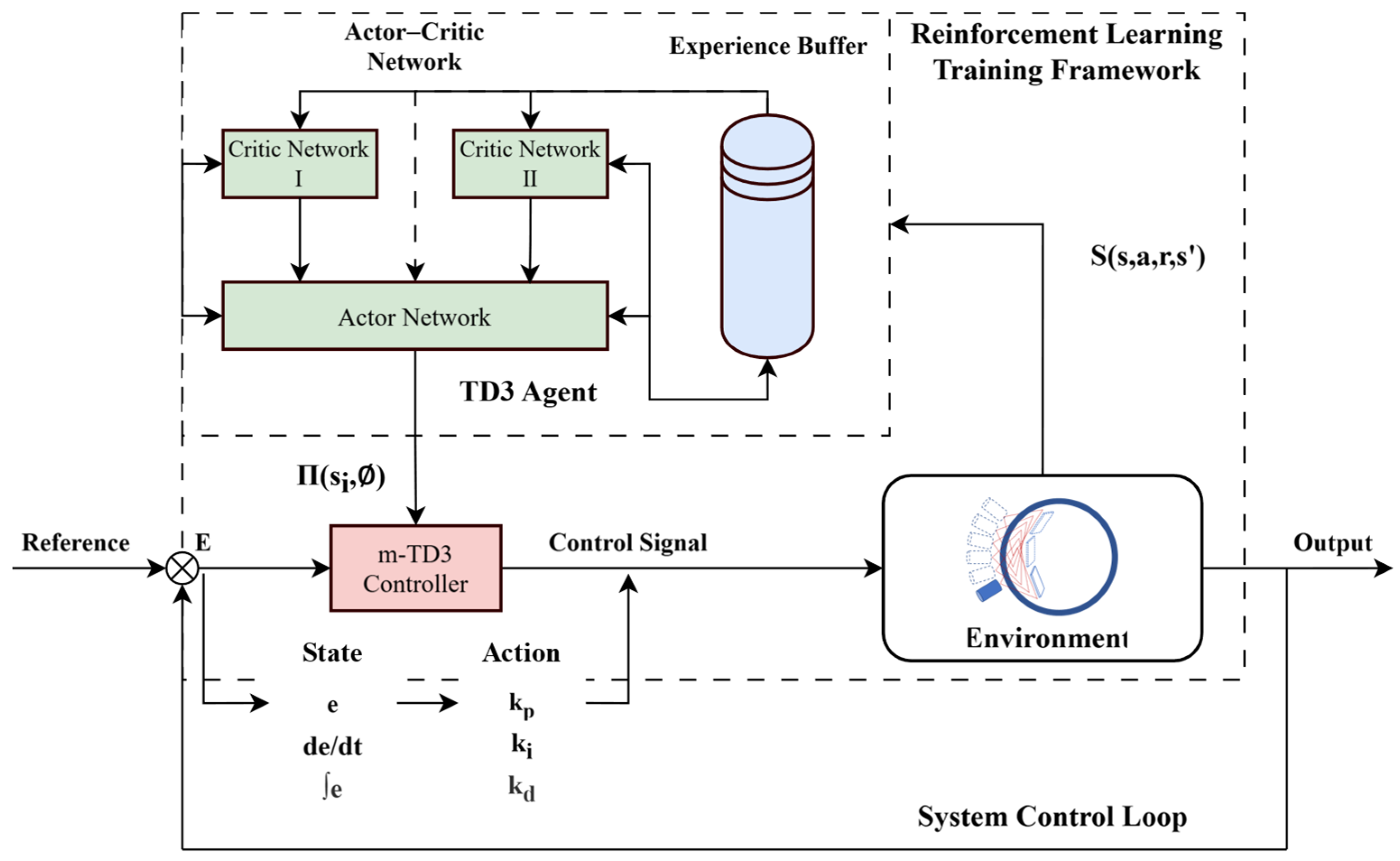
The TD3 algorithm employs an actor–critic architecture consisting of a single actor network and two critic networks. The actor generates actions based on observations of the external environment, while the critic networks assess these actions by evaluating their long-term impact. The agent learns through interactions within the state space S, receiving feedback via a reward function that aims to maximize the overall reward R.
TD3’s adaptive learning endows it with significant potential for actuator control and broader industrial applications. Accommodating dynamic system characteristics requires extensive training data and integration with conventional control strategies to ensure safety, while sufficient hardware performance may elevate costs. Nevertheless, TD3’s ability to process continuous, high-dimensional features makes it a promising solution for applications such as robotic control and industrial automation. The training process of the m-TD3 controller agent, along with the overall architecture of the actuator control system, is illustrated in Figure 3.

Figure 3.
Deep reinforcement learning (TD3)-based control framework for defect detection.
According to the universal approximation theory, a single hidden layer with enough neurons can approximate any continuous function defined on a compact set [30], so there is no need to use overly complex neural network structures when characterizing simple mapping relationships. In the deep neural network architecture designed in this paper, the actor network structure is , the number of neurons is , and the activation function of the fully connected layer is . The critic network structure design has a status path and strategy path, the structure is , , the number of neurons is , , the output generated by the splicing is propagated through the shared path , and the number of neurons is . is used in the activation function of the full-connection layer of the critic network. The reinforcement learning neural network architecture employed in this study is presented in Table 1.

Table 1.
Reinforcement learning agent neural network architecture.
A PMSM simulation model is established in the Simulink environment based on the principles of electromagnetism, dynamics, and control theory for permanent magnet synchronous motors. This model is applied to provide interaction data for the reinforcement learning agent. Additionally, the equivalent approximate transfer function can be derived from the motor parameters and the closed-loop speed control transfer formula, serving as an approximate model for experimental validation.
The following main points are considered in the design process of the actor–critic neural network:
- The shallow network will reduce the learning ability of the network, while the deep network will reduce the training speed and increase the computing cost consumption. More importantly, in the actual experiment, we found that the deep network will have a similar change trend in the output result due to the increase in the influence weight of the public part of the front end of the network before output differentiation, which will affect the actual effect. This is obviously not what we want to see, and the double hidden layer can achieve a good balance.
- The application of a tanh activation function in the front end of the actor network can limit the output of the hidden layer and avoid numerical explosion, which solves the instability caused by output oscillation in the actual training process. The additional relu after the output layer aims to limit the gain range of the PID controller.
- The critic network needs to integrate the current state and the output strategy of the actor network, and the output formula of the Q value is .
Given real-time constraints, deep reinforcement learning must balance computational complexity, overfitting risk, and training duration. For the agent’s design—particularly the actor network—excessive depth increases computational load and data requirements while slowing inference, whereas insufficient neurons weaken representational capacity. An optimal architectural balance is therefore essential.
The m-TD3 controller is a composite system integrating parallel , , and controllers, each with computational complexity comparable to a traditional PID controller, thereby ensuring real-time control signal outputs. At a higher level, the agent adaptively adjusts the control strategy with a decision execution period , ideally set to 0.01 s; current control devices can support the actor network’s output frequency at this interval. Through the fine-tuning of the neural network architecture to balance weight count and the optimization of the TD3 algorithm’s exploration strategy, the agent efficiently learns across diverse environmental conditions, substantially mitigating the risk of overfitting.
Furthermore, while extensive interaction and exploration with the environment are essential to achieving superior performance, a compromise in training time must be considered for tasks requiring rapid deployment.
We define the state space as , which sufficiently captures the controller’s required state for adaptive PID control. Redundant inputs not only inflate training costs and heighten overfitting risks but may also lead to dimensionality issues. To enhance adaptability across diverse scenarios, motor-specific information is deliberately excluded from the state vector. The actor network outputs the PID gains , thereby leveraging the agent’s learning capabilities to optimize response speed, steady-state error, and stability, ultimately maximizing the reward. Unlike conventional supervised learning, RL relies on iterative interactions with a pre-constructed environment and a reward function to maximize cumulative rewards. This training strategy significantly improves efficiency, reduces mechanical wear, and lowers industrial application costs.
3.2.2. Improved TD3 Algorithm
- Combination reward mechanism
Control effectiveness is evaluated by the integral of absolute error , with lower values indicating better performance. Accordingly, the TD3 reward function is defined as to minimize error. In practice, this is modified to by incorporating a gain coefficient to constrain reward magnitude and a time coefficient to mitigate high initial tracking errors—primarily due to environmental factors rather than agent decisions. Additionally, a heightened error penalty in later stages shifts focus toward minimizing steady-state error.
On this basis, the design idea of the reward function is improved, and the progress reward mechanism is added. When the agent makes progress in the control task, a certain degree of reward is given, . The idea of the progress reward mechanism comes from the fact that an agent performs poorly when inputs state at a certain time, which is more likely to be caused by a bad decision at a previous time in an actual control task. It is obviously unfair to give a poor evaluation of the decision in the current state. Perhaps the agent has made the best decision in the present moment. At the same time, if the intelligent body keeps achieving higher evaluation in the process of interacting with the environment, it can also eventually learn the ideal strategy.
In the actual training process, we find that the independent use of an evaluation reward or progress reward can realize the training of the agent, to achieve the purpose of adaptive control. However, there are differences in the effects of the two reward mechanisms. The training speed of the agent when the progress reward is applied is notably faster than the evaluation reward, and the response speed of the adaptive controller is also faster. However, the effect of eliminating steady-state error is not as ideal as that when the evaluation reward is applied. Therefore, applying the combination reward mechanism can synthesize the advantages of both. The formula is as follows:
where the evaluation coefficient and progress coefficient can be used to adjust the degree of emphasis on the two different rewards in the training process.
- b.
- Security constraint mechanism
In the process of agent training, especially in the early stage of training, there will be system instability caused by wrong decisions, which can even cause training to stop or system collapse. Therefore, it is very important to introduce a security constraint mechanism. We believe that the security constraint mechanism is implemented in two ways: rule punishment and behavior suppression. Rule punishment is to give a large reward punishment when the agent adopts a policy that does not comply with the security rules, to inhibit the agent’s tendency to display extreme behaviors. The means of achieving this is to add a large rule penalty term to the reward function. Behavior suppression is to immediately stop the subsequent training process of the round when the agent adopts an extreme strategy that results in the state of the controlled system exceeding its anticipated, acceptable limits or exhibits a propensity to violate established rules, so as to avoid the unstable situation of the system caused by the agent’s wrong decision under the existing strategy in advance and avoid serious consequences. In addition, adjusting the neural network structure, such as by using the activation function, is also a strategy for avoiding displays of excessive behavior by the agent, but it limits the learning ability of the actor–critic network to a certain extent, so a certain balance needs to be struck between the two.
The proposed security constraint mechanism establishes explicit safety rules and terminates the current training episode when violations occur, imposing substantial penalties. For motor control tasks, these rules enforce parameters such as controller output , Q-axis current , and temperature T remaining within safe ranges.
3.2.3. m-TD3 Composite Controller Based on CP-MPA
In this paper, the m-TD3 composite controller is developed using the CP-MPA swarm intelligence algorithm to optimize its structure by integrating deep reinforcement learning with modern control theory. The inherent simplicity and universality of feedback control have established it as the industrial standard, while feedforward control plays a pivotal role in modern control frameworks. The synergistic integration of feedback error compensation and feedforward tracking effectively enhances control accuracy.
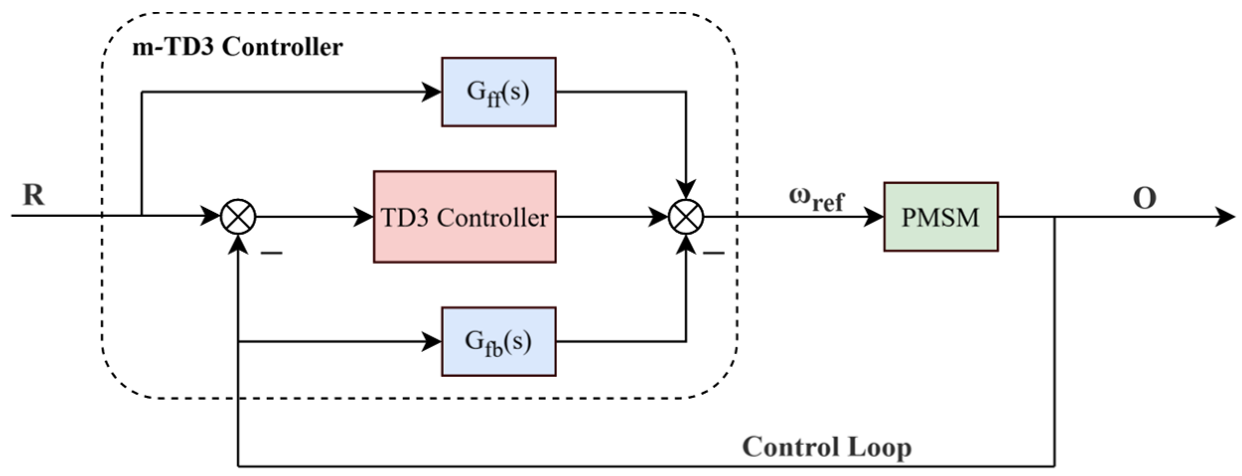
Leveraging PMSM control characteristics, a feedforward tracking controller is integrated with the position-loop reinforcement learning TD3 controller, while a feedback compensation controller is incorporated into the speed-loop feedback circuit. Together, these form the speed-loop control signal source, known as the m-TD3 composite controller. The system architecture is depicted in Figure 4.
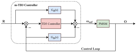
Figure 4.
Structure of m-TD3 composite controller based on CP-MPA.
The transfer formula of the feedforward tracking controller and feedback compensation controller is [31]
The feedforward tracking controller can improve the tracking performance of the controller for low-frequency signals and improve the control accuracy. The feedback compensation controller can improve the stability margin and robustness of the system, and the reinforcement learning TD3 controller can compensate for the tracking error.
Let the transfer function of the TD3 controller be , and the transfer function of the motor part be simplified to ; that is, for the speed ring composed of PMSMs, there is . The output control signal formula of the m-TD3 controller is as follows:
The open-loop transfer function is analyzed:
The closed-loop transfer function of the m-TD3 compound control position loop is obtained as follows:
The m-TD3 composite controller features four tunable parameters—, , , and —that critically impact performance. However, traditional transfer function analysis (focusing on zeros, poles, gains, cutoff frequencies, and stability margins) is inapplicable to reinforcement learning-based adaptive controllers.
In this paper, we propose a meta-heuristic, population-based, deep-sea predator algorithm (CP-MPA) that leverages swarm intelligence to optimize controller performance by determining optimal parameter configurations. The Marine Predator Algorithm (MPA) draws inspiration from the optimal foraging strategies of marine predators, emulating predator–prey behaviors and integrating Levy flight and Brownian motion in both sparse and dense environments to effectively search for optimal solutions [32].
The MPA divides the whole optimization process into three stages: low-speed ratio, unit-speed ratio, and high-speed ratio. Predators and prey adopt different updating strategies at different stages.
- Update formula for the exploration process incorporating Brownian motion:
- Update formula for the exploitation process incorporating Lévy flight:where is the prey matrix, is the predator matrix, is the global step size, is the exploration variable in [0,1), is the Brownian motion variable, is the convergence variable, and is the Levy flight variable. In addition, the MPA applies FAD perturbation to the prey matrix to further improve the exploration ability of the algorithm [32].
To enhance the optimization capability of the MPA and optimize the m-TD3 composite controller, this study introduces the following improvements to the MPA, proposing CP-MPA:
- Chaotic initialization: Because the initial population critically affects optimization, random initialization can yield uneven coverage and restricted exploration. Chaotic initialization ensures more uniform coverage and enhances global exploration:where is the chaotic sequence generated by chaotic mapping, and its value is in the range of . An initialization and chaos factor are required, and the chaotic sequence is generated by the formula [33]
- Predator population mechanism: The predator matrix in Reference [32] is repeatedly copied from top predators, and is the same. In the actual natural environment, predator groups should also have individuality; that is, there should be individual differences among predators. At the same time, there is also an apex predator, the leader of the predator population. The individual behavior of the predator should be influenced by the decisions of both the prey and the leader. Therefore, this paper proposes an MPA based on the predator population mechanism. The improved predator population behavior is defined by the formula as follows:
In this formula, is the tracking process of the predator individual to the prey, and the optimal individual fitness value is recorded, that is, the position where the prey is most likely to appear. is the tracking process of the top predator, is the same, and the position of the global optimal fitness value is recorded. is the social factor of the predator population. The larger is, the stronger sociality is, and the more the predator individual is affected by the population. is the predator tracking process affected by the population. The improved MPA is updated by .
CP-MPA utilizes chaotic initialization to generate a uniformly distributed initial population, enhancing global exploration and reducing premature convergence. This strategy not only accelerates convergence toward the optimal solution but also improves stability in high-dimensional scenarios. The addition of a predator population mechanism preserves individual distinctions and refines local search, maintaining population diversity throughout the iterative process. Compared with the conventional MPA, CP-MPA better balances self-learning with the exploitation of optimal solutions, thereby mitigating premature convergence. Moreover, since its offline iterative learning is performed on high-performance hardware, the extra computational cost does not burden real-time control. Consequently, CP-MPA effectively optimizes the m-TD3 controller’s performance.
3.2.4. Deployment of the m-TD3 Composite Controller
The agent is trained to generate a policy model, and the reinforcement learning policy model is saved in .mat format. In the defect detection system, the embedded control center is responsible for controlling multiple actuators, and the m-TD3 controller is deployed on this platform. Currently, the controller is planned to run on an STM32F429VET6 chip (STMicroelectronics, Switzerland) based on the ARM Cortex-M4 architecture, operating at a main frequency of 180 MHz. The policy model, together with the control logic, must be compiled into C code through a suitable compiler and integrated into the control tasks. After compilation, a cross-compilation toolchain is used to flash the resulting binary onto the embedded control center.
The embedded control center employs the FreeRTOS real-time operating system, whose task scheduling mechanism ensures real-time control signals for multiple actuators. At the lower level, the parallel control modules , , and in the m-TD3 controller form a composite controller capable of the real-time output of control signals, while the agent’s policy is updated every 0.01 s within a FreeRTOS task. The method of deploying the learned control policy on the embedded control center largely resembles that of general neural network deployment; nevertheless, it imposes certain performance demands on the embedded hardware platform. Code optimization or neural network quantization can be adopted to mitigate resource usage. Furthermore, a higher-performance hardware platform can accommodate more frequent controller policy updates, albeit at the expense of increased hardware cost.
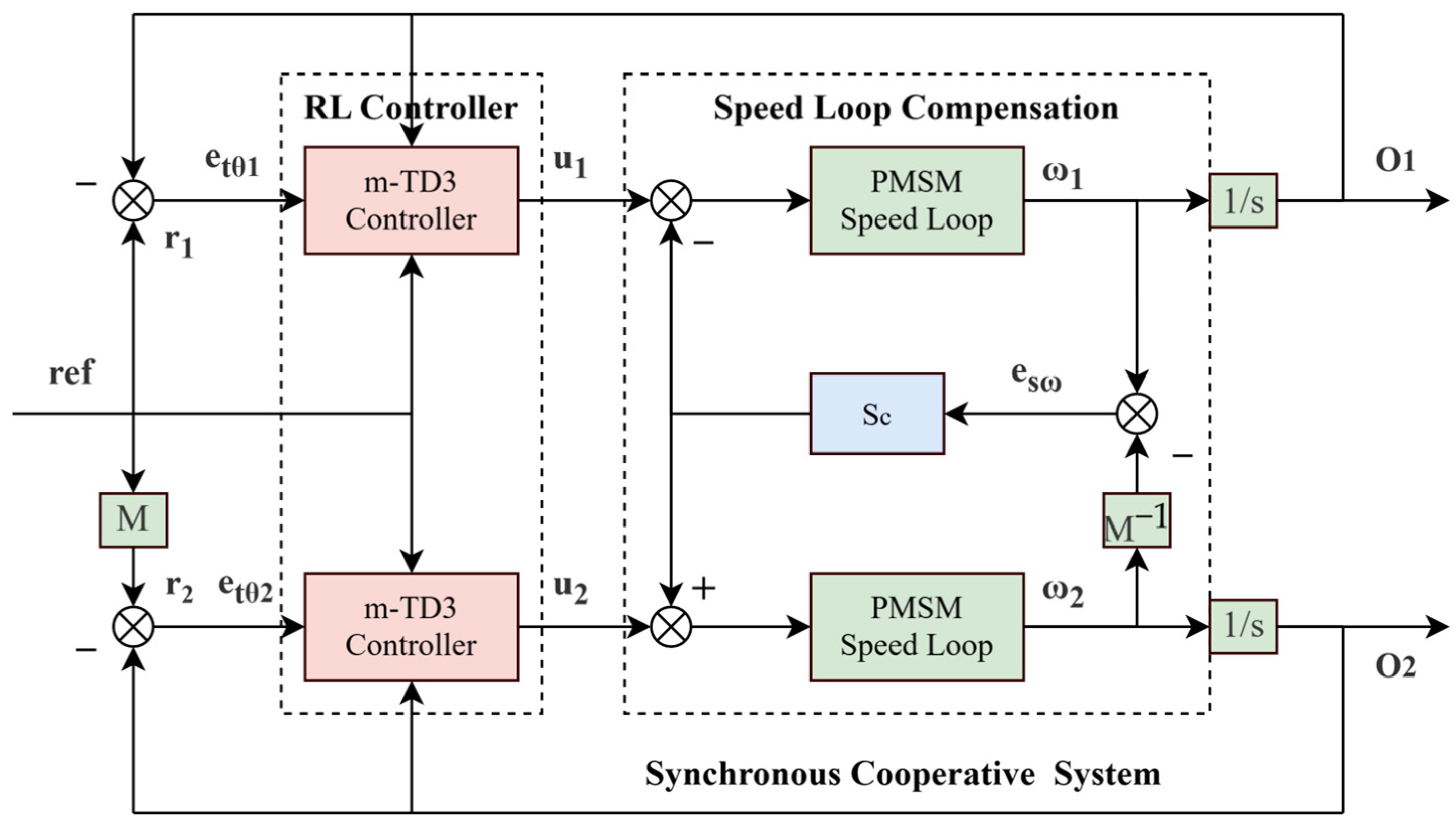
3.3. Synchronous Cooperative Motion Compensator
The spherical shell weld defect detection system of manned submersed vehicles is based on the synchronous cooperative motion of the CNT cold-cathode X-ray source and detector, and the motion synchronization accuracy has an important impact on the subsequent 3D image reconstruction. In this paper, a synchronous cooperative motion compensator for the detection system is designed to realize the high-precision synchronous motion of the detection system. The synchronous cooperative control structure of the defect detection system is illustrated in Figure 5.
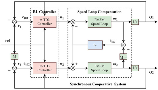
Figure 5.
Synchronous cooperative control structure.
The synchronous cooperative motion compensator acts on the speed ring, and the compensator transfer function is as follows:
where and are compensation coefficients, the introduction of the compensator will affect the independent motion and synchronous motion of the system at the same time, and is the length of the sliding window, which can effectively suppress the influence of integer multiples of frequency harmonics. , , is the phase compensation frequency, and is the frequency multiplication factor. Combined with the lead correction, the response retardation caused by harmonic suppression can be compensated and the phase margin of the compensator can be improved. In order to obtain a more ideal control effect of the detection system, CP-MPA can be applied to optimize the parameters, and the fitness function is designed as follows:
In this formula, and represent the tracking errors of the CNT X-ray source and the detector, respectively. denotes the position synchronization error, refers to the speed synchronization error, and is the synchronization weight, indicating the level of attention the detection system places on synchronized motion. is the speed synchronization weight representing the degree of attention that the detection system pays to speed synchronization. By adjusting , can select different system control optimization strategies.
4. Experiment
In this paper, the defect detection system drive motor control model is constructed in the MATLAB R2024b and Simulink 24.2 environment as a deep reinforcement learning interactive environment to train the agent. Combined with CP-MPA optimization and 2-DOF control, the m-TD3 composite controller is constructed for driving motor control. Simulation experiments verify the effectiveness of the m-TD3 composite controller in the first-order unstable system, second-order complex unstable system, equivalent approximate PMSM linear system, and simulated PMSM control system scenarios. At the same time, the control effects of the m-TD3 composite controller, MPA-optimized PID, two-degree-of-freedom m-PID controller, and TD3 reinforcement learning controller are compared. The quantitative metrics utilized for evaluating the controller performance in the experimental analysis are summarized in Table 2. The training hyperparameters adopted for the reinforcement learning agent are detailed in Table 3.
Table 2.
Quantitative formulas of control effect evaluation indexes.
Table 3.
Deep reinforcement learning agent training parameters.
4.1. Linear System Simulation Experiments
In this paper, the performance of the m-TD3 composite controller is verified in the first-order unstable system, the second-order complex unstable system, and the equivalent approximate PMSM linear system.
Transfer function of first-order unstable system:
Transfer function of second-order complex unstable system:
In the equivalent approximation process, for the speed-loop PI controller, , , for the current-loop PI controller, , , . Based on the permanent magnet synchronous motor parameters listed in Table 4, the equivalent approximation formula of the PMSM speed loop is derived as follows:
Table 4.
Permanent magnet synchronous motor parameters.
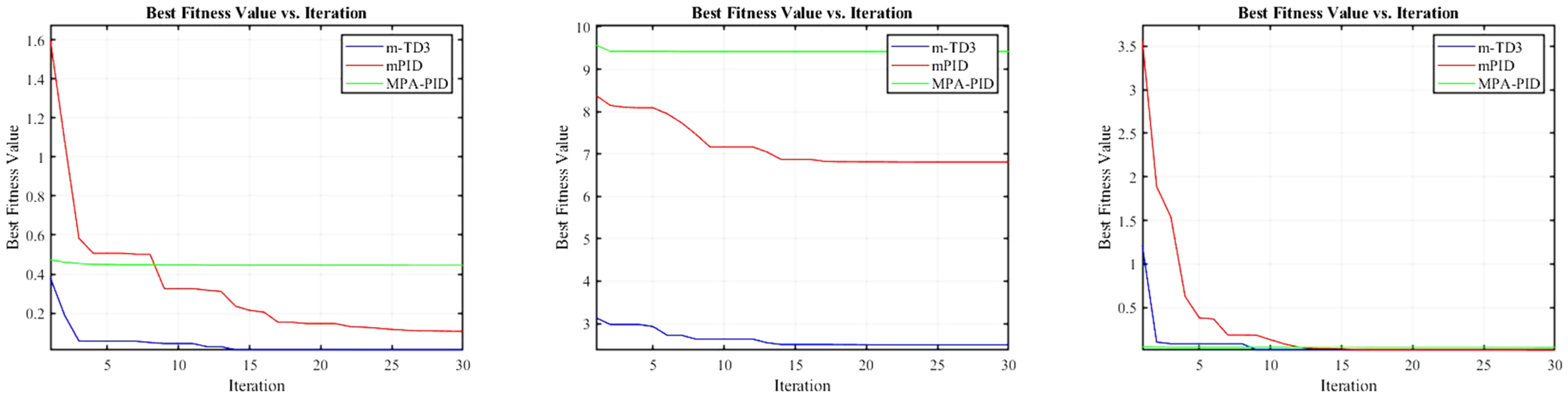
In the early stage of training, the agent will extensively explore the policy, so the reward will oscillate to a certain extent and become stable after a certain training round, at which time the agent learns certain rules and gradually achieves better performance. In terms of coping with control-related problems, the introduction of the combined reward mechanism effectively improves the efficiency of agent learning. Most existing studies apply a single evaluation coefficient, which requires a large number of training episodes. In some cases, the agent may even be trapped in the sub-optimal strategy space. We believe that using even a single improvement coefficient is more optimal when considering the fitting efficiency and the pros and disadvantages of the strategy.
Table 5 shows the optimal parameter configuration and fitness values of MPA-optimized PID, the two-degree-of-freedom m-PID controller, and the m-TD3 composite controller after complete iterative optimization in the first-order unstable system, second-order complex unstable system, and equivalent approximate PMSM linear system. Figure 6 illustrates the variation trend of the fitness value with respect to the number of iterations. Based on the of the fitness function, a tiny parameter is added to prevent system instability caused by the parameter being too large. It can be seen in Table 5 that the m-TD3 composite controller has obtained the lowest fitness value in three different unstable linear systems, and it can be preliminarily assumed that the m-TD3 composite controller has the best control performance.
Table 5.
The optimal parameters and optimal fitness value of the linear systems after iterative optimization.
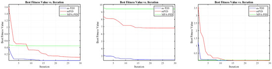
Figure 6.
Variation trend in fitness for iterative optimization of linear systems.
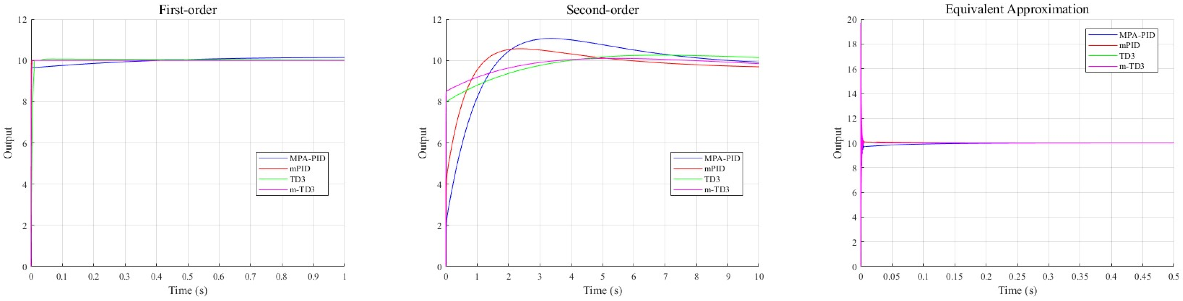
Figure 7 illustrates that for first-order unstable transfer functions and their approximate equivalents, an ideal control effect is achieved with the exception of the MPA-PID approach. The presence of a minor third-order term in the approximate equivalent transfer function induces a pronounced oscillatory overshoot in the response curve. In contrast, significant differences are observed in the control performance of the reinforcement learning method applied to second-order unstable systems. Specifically, the agent’s control strategy exhibits rapid response during the acceleration phase, transitioning to slower approximation as the response curve approaches the control signal. This rapid phase underpins improvements in and , while the subsequent slow phase ensures a reduced and . These results underscore the considerable advantages of the combined reinforcement learning agent control method.
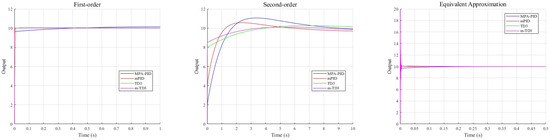
Figure 7.
MPA-PID, mPID, TD3, and m-TD3 controller linear system output.
Table 6 shows the control process evaluation indexes of MPA-optimized PID, the two-degree-of-freedom m-PID controller, the TD3 controller, and the m-TD3 composite controller. For the first-order unstable system, the m-TD3 composite controller achieves the optimal level of steady-state error and overshoot, the achieves a sub-optimal level, and the m-PID controller has the fastest response speed and the lowest . Because of the design of reward function , the intelligent agent tends to apply the strategy of low steady-state error. When dealing with simple systems, does not have a significant advantage but still achieves excellent performance. In the control of second-order complex unstable systems, the m-TD3 composite controller is much better than the other three controllers in terms of various evaluation indexes, which shows its potential in dealing with complex situations. In the experiment of the approximate equivalent system, the m-TD3 composite controller achieves optimal performance in , , and , and the controller applying the reinforcement learning method has excellent performance in and . The indexes are close except for that of MPA-PID, but the overall control effect of MPA-PID is far worse than that of the other three controllers. Overall, the m-TD3 composite controller proposed in this paper has the best control effect in linear system simulation.
Table 6.
MPA-PID, mPID, TD3, and m-TD3 controller linear system control effect evaluation: quantified values.
4.2. PMSM Control System Simulation Experiment
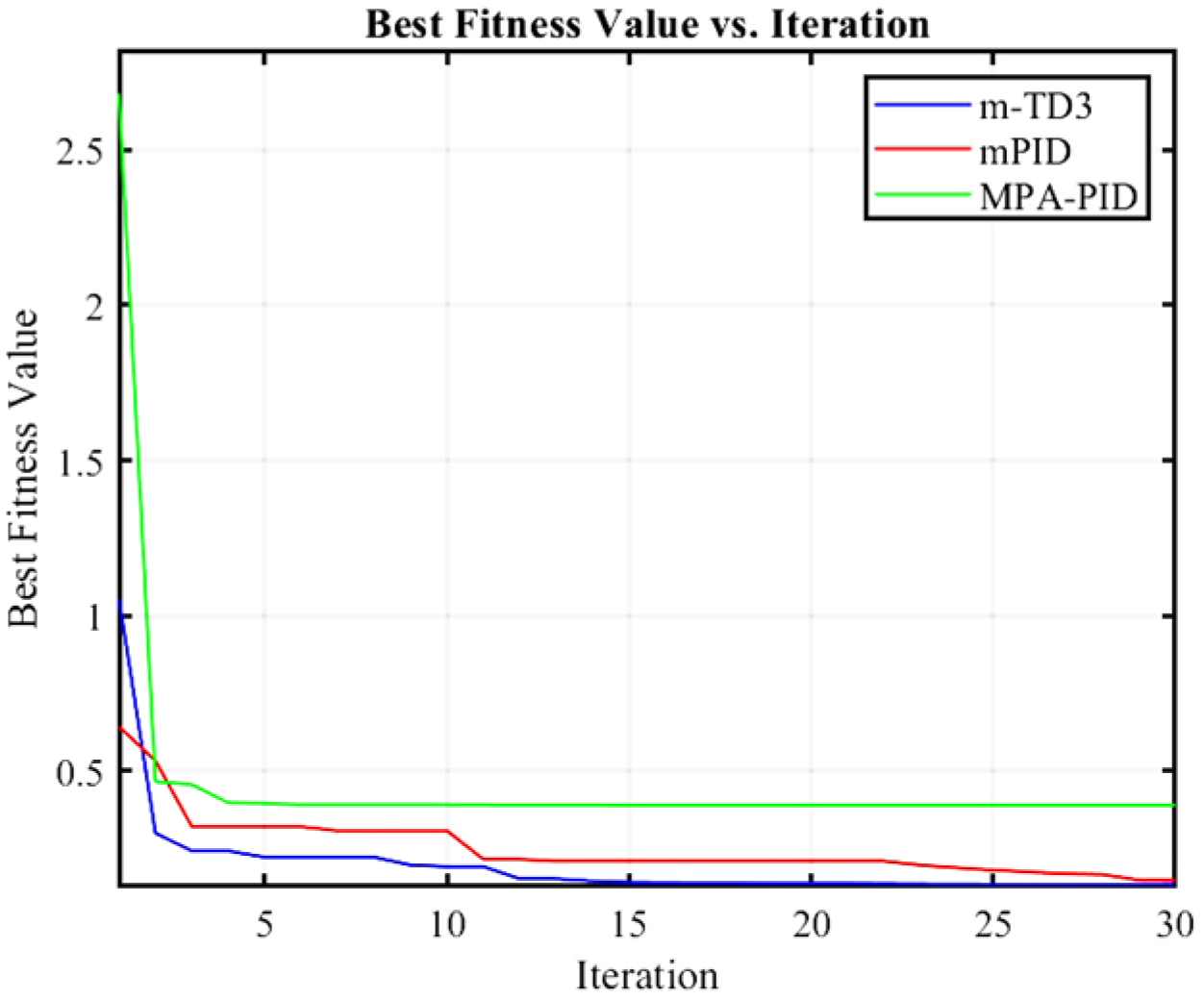
Figure 8 shows the optimization results of three different controllers, among which the optimal fitness of MPA-PID is 0.3898, that of mPID is 0.1461, and that of m-TD3 is 0.1343. Therefore, the m-TD3 composite controller also achieves optimal fitness in the simulation of the PMSM control system. At this time, the parameters , , , and of the m-TD3 composite controller are 0.75158, 3.4796, 0.48245, and 1.9657, respectively.

Figure 8.
Variation trend in fitness for iterative optimization of PMSM control system.
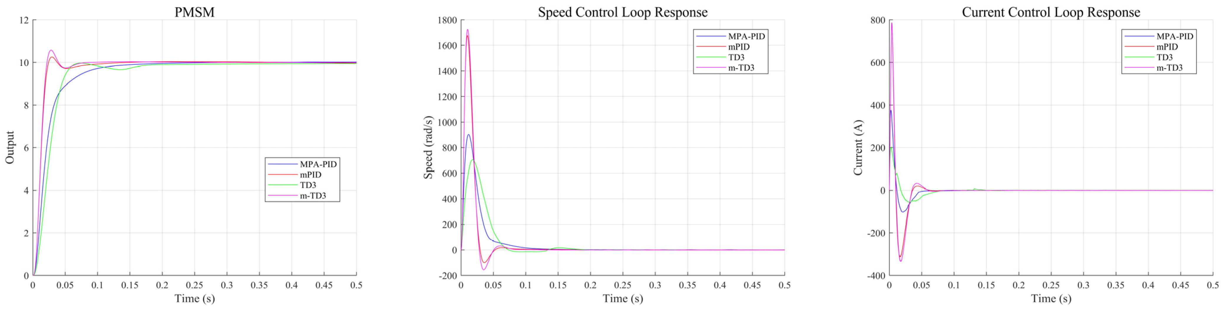
As can be seen from Figure 9, both TD3 and MPA-PID are relatively stable control strategies, which can effectively suppress overshoot. The high-speed tracking stage of TD3 will last longer, and correspondingly, there will be more efficient deceleration behavior, resulting in a slight drop and then steady tracking. This control strategy is learned by the agent and is very different from traditional PID. The high-speed phase lasting longer will make the agent respond faster in the case of a large mutation, and the two-stage slow approach will also make the steady-state error more ideal for a long time. The introduction of the feedforward tracking controller and feedback compensation controller greatly improves tracking efficiency. It can be seen from the output of the speed loop and current loop that the composite controller has a more aggressive strategy with higher speed and current fluctuations. The faster convergence rate in the m-TD3 composite controller also makes the advantage of the agent control strategy at the steady-state error level manifest.
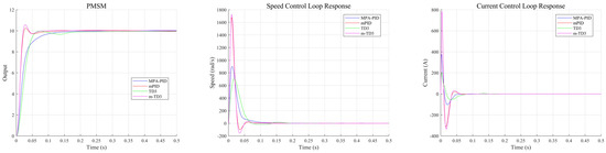
Figure 9.
MPA-PID, mPID, TD3, and m-TD3 controller PMSM control system output.
The quantified evaluation results of control performance for the MPA-PID, mPID, TD3, and m-TD3 controllers in the PMSM control system are presented in Table 7. In the simulation environment of 0.5 s, the m-TD3 composite controller achieves optimal performance in terms of , , and , while the TD3 controller achieves optimal performance and avoids overshoot to the greatest extent. The steady-state error level of the m-TD3 composite controller is excellent, only 54.86% of that of the sub-optimal MPA-PID. In the simulation environment of 2 s, the m-TD3 composite controller has excellent performance in terms of the index, which is only 51.46% of that of the second-best controller, while the TD3 controller has the lowest steady-state error. In summary, the reinforcement learning control strategy has great advantages in PMSM control system simulation experiments, especially in , , and . In terms of overshoot, the pure TD3 controller is the best.
Table 7.
MPA-PID, mPID, TD3, and m-TD3 controller PMSM control system control effect evaluation quantified values.
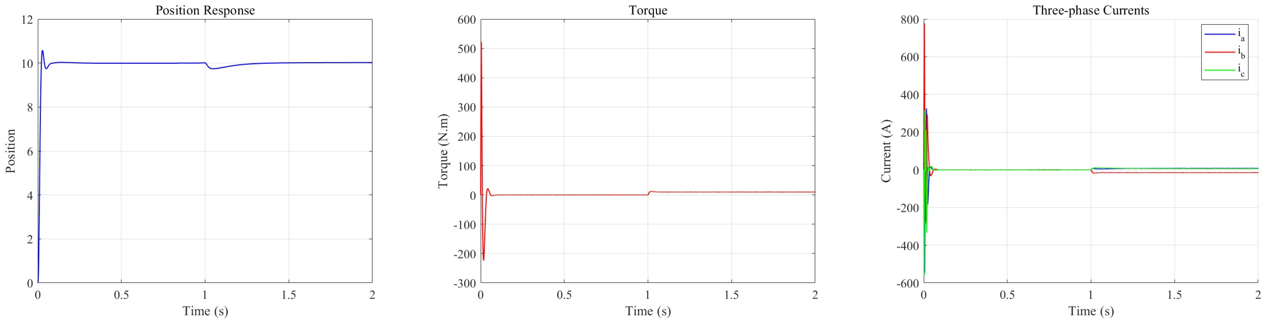
Figure 10 illustrates that upon the application of a load of at 1 s, the PMSM response exhibits a transient decline. The m-TD3 composite controller effectively mitigates this drop and rapidly compensates for the ensuing tracking error. Specifically, the maximum disturbance attenuation is approximately 0.261, with a compensation time of about 0.414 s. An analysis of the torque output further reveals that under no-load conditions, the torque tracking control signal stabilizes at zero during a steady state. Conversely, when a load disturbance is introduced, the controller promptly modulates the torque output to counteract the transient deviation and subsequently maintains a consistent torque level to re-establish stability. Additionally, the three-phase current outputs conform closely with theoretical predictions. These findings substantiate the robust control performance of the m-TD3 composite controller under load disturbances.
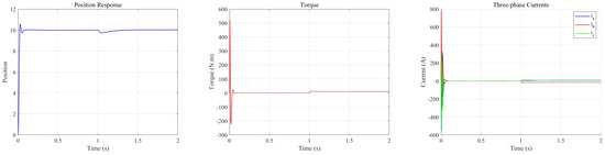
Figure 10.
Output response of the m-TD3-based PMSM control system under load mutation.
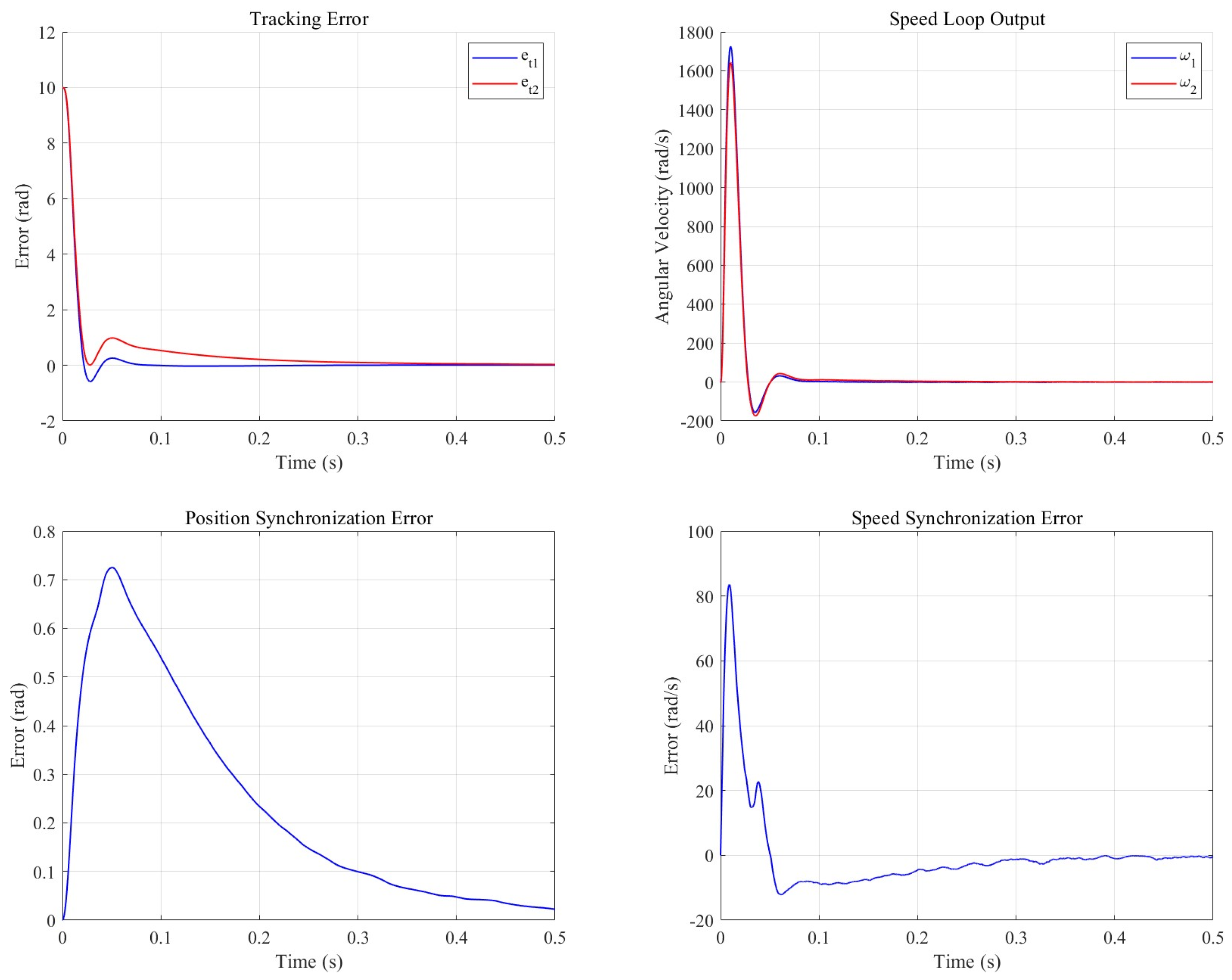
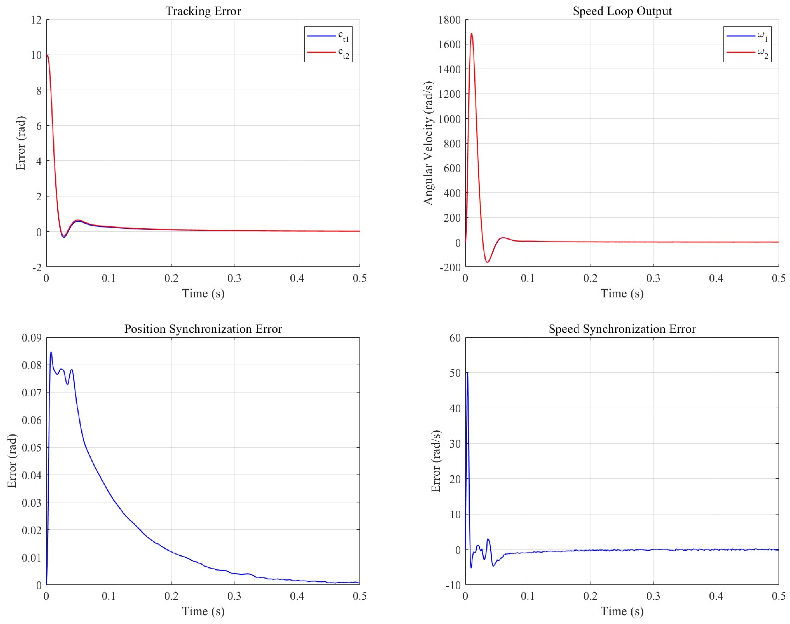
The synchronous cooperative motion compensator is set to 10, is set to , is set to 2, after CP-MPA optimization is 98, is set to 11,230, and the cooperative control model is built in Simulink. One of the two motors is a no-load motor, and the other is set to load . The control effect is shown in the subsequent figure.
As illustrated in Figure 11 and Figure 12, the synchronous cooperative motion compensator effectively mitigated the motion discrepancies between the dual motors in the defect detection system. Specifically, the positional synchronization error was reduced by 92.4%, with its peak value decreasing by 88.3%, while the speed synchronization error was curtailed by 86.7% and its peak value by 40%. Furthermore, the compensator enhanced the tracking performance of the load-interference motor, as evidenced by a reduction of 0.05103 in its integrated absolute error (IAE), although the IAE for the no-load motor exhibited an increase of 0.04118.
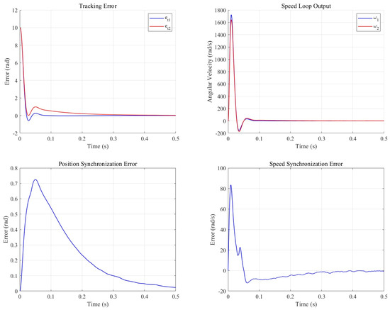
Figure 11.
Nonsynchronous cooperative motion compensation system output.
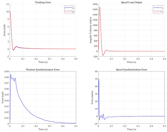
Figure 12.
Synchronous cooperative motion compensation control system output.
The efficient actuator control performance of the m-TD3 controller has been validated. When integrated with a collaborative motion compensator that suppresses multi-actuator cooperative errors, it provides comprehensive and precisely localized image information for the defect detection system, thereby enhancing both detection efficiency and accuracy. Conversely, the m-TD3 controller necessitates a higher-performance hardware platform, which increases hardware costs. Moreover, while a reinforcement learning agent can achieve optimal decision-making capabilities with sufficient training and data, tasks requiring rapid deployment demand a careful balance regarding training time.
5. Conclusions
In this paper, an m-TD3 composite controller integrating deep reinforcement learning with a swarm intelligence algorithm is proposed. Specifically, the MPA is enhanced via chaotic initialization and a predator population mechanism, and combined with a composite reward mechanism to refine the TD3 agent’s structural design, thereby improving controller performance. Meanwhile, a synchronous co-compensator is introduced alongside the m-TD3 composite controller to form a complete control scheme for the defect detection system. Finally, simulations in both linear and defect detection system environments demonstrate the feasibility and effectiveness of the proposed scheme.
Author Contributions
Conceptualization, Y.C. and L.Z.; methodology, Y.C. and L.Z.; software, Y.C.; validation, Y.C., Z.L. and L.Z.; investigation, Y.C.; resources, L.Z.; data curation, Y.C. and X.C.; writing—original draft preparation, Y.C.; writing—review and editing, Y.C. and Z.L.; supervision, L.Z. and Z.L.; project administration, L.Z.; funding acquisition, L.Z. and Z.L. All authors have read and agreed to the published version of the manuscript.
Funding
Funding for this work was provided by the National Key R&D Program of China (2021YFC 2802000).
Data Availability Statement
Data will be made available on request.
Acknowledgments
We would like to thank the above funders for their support.
Conflicts of Interest
The authors declare no conflicts of interest.
References
- Miller, T.J.E. Brushless Permanent-Magnet and Reluctance Motor Drives; IEEE Press: New York, NY, USA, 1989. [Google Scholar]
- Li, J.; Yu, J.J.; Chen, Z. A Review of Control Strategies for Permanent Magnet Synchronous Motor Used in Electric Vehicles. Appl. Mech. Mater. 2013, 321–324, 1679–1685. [Google Scholar] [CrossRef]
- Sato, D.; Itoh, J.-I. Open-loop control for permanent magnet synchronous motor driven by square-wave voltage and stabilization control. In Proceedings of the 2016 IEEE Energy Conversion Congress and Exposition (ECCE), Milwaukee, WI, USA, 18–22 September 2016; pp. 1–8. [Google Scholar] [CrossRef]
- Blaschke, F. The principle of field orientation as applied to the new TRANSVECTOR closed loop control system for rotating field machines. Siemens Rev. 1972, 34, 217–220. [Google Scholar]
- Pillay, P.; Krishnan, R. Modeling, simulation, and analysis of permanent-magnet motor drives. I. The permanent-magnet synchronous motor drive. IEEE Trans. Ind. Appl. 1989, 25, 265–273. [Google Scholar] [CrossRef]
- Takahashi, I.; Noguchi, T. A New Quick-Response and High-Efficiency Control Strategy of an Induction Motor. IEEE Trans. Ind. Appl. 1986, IA-22, 820–827. [Google Scholar] [CrossRef]
- Minorsky, N. Directional stability of automatically steered bodies. J. Am. Soc. Nav. Eng. 1922, 34, 280–309. [Google Scholar] [CrossRef]
- Utkin, V. Variable structure systems with sliding modes. IEEE Trans. Autom. Control 1977, 22, 212–222. [Google Scholar] [CrossRef]
- Zadeh, L.A. Fuzzy sets. Inf. Control 1965, 8, 338–353. [Google Scholar] [CrossRef]
- Zadeh, L.A.; Yuan, B.; Klir, G.J. Fuzzy Sets, Fuzzy Logic, and Fuzzy Systems; Selected Papers by Lotfi A. Zadeh; World Scientific Publishing Co., Inc.: Hackensack, NJ, USA, 1996. [Google Scholar]
- Visioli, A. Tuning of PID controllers with fuzzy logic. IEE Proc. Control Theory Appl. 2001, 148, 1–8. [Google Scholar] [CrossRef]
- Mohammed, N.F.; Song, E.; Ma, X.; Hayat, Q. Tuning of PID controller of synchronous generators using genetic algorithm. In Proceedings of the 2014 IEEE International Conference on Mechatronics and Automation, Tianjin, China, 3–6 August 2014; pp. 1544–1548. [Google Scholar] [CrossRef]
- Gaing, Z.-L. A particle swarm optimization approach for optimum design of PID controller in AVR system. IEEE Trans. Energy Convers. 2004, 19, 384–391. [Google Scholar] [CrossRef]
- Bhattacharyya, D.; Ray, A.K. Stepless PWM speed control of AC motors: A neural network approach. Neurocomputing 1994, 6, 523–539. [Google Scholar] [CrossRef]
- Mao, Z.; Kobayashi, R.; Nabae, H.; Suzumori, K. Multimodal Strain Sensing System for Shape Recognition of Tensegrity Structures by Combining Traditional Regression and Deep Learning Approaches. IEEE Robot. Autom. Lett. 2024, 9, 10050–10056. [Google Scholar] [CrossRef]
- Peng, Y.; Yang, X.; Li, D.; Ma, Z.; Liu, Z.; Bai, X.; Mao, Z. Predicting flow status of a flexible rectifier using cognitive computing. Expert Syst. Appl. 2025, 264, 125878. [Google Scholar] [CrossRef]
- Sutton, R.S. Learning to predict by the methods of temporal differences. Mach. Learn. 1988, 3, 9–44. [Google Scholar] [CrossRef]
- Mnih, V.; Kavukcuoglu, K.; Silver, D.; Graves, A.; Antonoglou, I.; Wierstra, D.; Riedmiller, M. Playing Atari with Deep Reinforcement Learning. arXiv 2013, arXiv:1312.5602. [Google Scholar]
- Mnih, V.; Badia, A.P.; Mirza, M.; Graves, A.; Lillicrap, T.; Harley, T.; Silver, D.; Kavukcuoglu, K. Asynchronous Methods for Deep Reinforcement Learning. In Proceedings of the 33rd International Conference on Machine Learning, New York, NY, USA, 19–24 June 2016; pp. 1928–1937. [Google Scholar]
- Lillicrap, T.P.; Hunt, J.J.; Krizhevsky, A.G.; Silver, D.; Salakhutdinov, R. Continuous control with deep reinforcement learning. In Proceedings of the International Conference on Learning Representations (ICLR), San Juan, Puerto Rico, 2–4 May 2016. [Google Scholar]
- Schulman, J.; Wolski, F.; Dhariwal, P.; Radford, A.; Klimov, O. Proximal Policy Optimization Algorithms. arXiv 2017, arXiv:1707.06347. [Google Scholar]
- Fujimoto, S.; van Hoof, H.; Meger, D. Addressing Function Approximation Error in Actor-Critic Methods. In Proceedings of the 35th International Conference on Machine Learning, Stockholm, Sweden, 10–15 July 2018; pp. 1582–1590. [Google Scholar]
- Haarnoja, T.; Zhou, A.; Abbeel, P.; Levine, S. Soft Actor-Critic: Off-Policy Maximum Entropy Deep Reinforcement Learning with a Stochastic Actor. In Proceedings of the 35th International Conference on Machine Learning, Stockholm, Sweden, 10–15 July 2018; pp. 1861–1870. [Google Scholar]
- Shuprajhaa, T.; Sujit, S.K.; Srinivasan, K. Reinforcement learning based adaptive PID controller design for control of linear/nonlinear unstable processes. Appl. Soft Comput. 2022, 128, 109450. [Google Scholar] [CrossRef]
- Dogru, O.; Velswamy, K.; Ibrahim, F.; Wu, Y.; Sundaramoorthy, A.S.; Huang, B.; Xu, S.; Nixon, M.; Bell, N. Reinforcement Learning Approach to Autonomous PID Tuning. In Proceedings of the 2022 American Control Conference (ACC), Atlanta, GA, USA, 8–10 June 2022; pp. 2691–2696. [Google Scholar] [CrossRef]
- Bloor, M.; Ahmed, A.; Kotecha, N.; Mercangöz, M.; Tsay, C.; del Río-Chanona, E.A. Control-Informed Reinforcement Learning for Chemical Processes. Ind. Eng. Chem. Res. 2024, 64, 4966–4978. [Google Scholar] [CrossRef]
- Zhu, B.; Zhang, Y.; Xu, P.; Song, S.; Jiao, S.; Zheng, X. A dual-motor cross-coupling control strategy for position synchronization. J. Harbin Univ. Sci. Technol. 2022, 27, 114–121. [Google Scholar] [CrossRef]
- Zhang, Y. Research on X-ray Source Optimization and System Control Method for Spherical Shell Weld Inspection. Master’s Thesis, Southeast University, Nanjing, China, 2022. [Google Scholar]
- Yuan, L.; Hu, B.; Wei, K.; Chen, S. Principles of Modern Permanent Magnet Synchronous Motor Control and MATLAB Simulation; Beihang University Press: Beijing, China, 2016. [Google Scholar]
- Cybenko, G. Approximation by superpositions of a sigmoidal function. Math. Control Signals Syst. 1989, 2, 303–314. [Google Scholar] [CrossRef]
- Shi, R.; Liu, W.; Wang, G.; Lan, C.; Xu, M. Improved voltage regulation strategy for three-phase PWM rectifier based on two-degree-of-freedom PID. Electr. Power Eng. Technol. 2023, 42, 149–156+178. [Google Scholar]
- Faramarzi, A.; Heidarinejad, M.; Mirjalili, S.; Gandomi, A.H. Marine Predators Algorithm: A nature-inspired metaheuristic. Expert Syst. Appl. 2020, 152, 113377. [Google Scholar] [CrossRef]
- May, R.M. Simple mathematical models with very complicated dynamics. Nature 1976, 261, 459–467. [Google Scholar] [CrossRef] [PubMed]
Disclaimer/Publisher’s Note: The statements, opinions and data contained in all publications are solely those of the individual author(s) and contributor(s) and not of MDPI and/or the editor(s). MDPI and/or the editor(s) disclaim responsibility for any injury to people or property resulting from any ideas, methods, instructions or products referred to in the content. |
© 2025 by the authors. Licensee MDPI, Basel, Switzerland. This article is an open access article distributed under the terms and conditions of the Creative Commons Attribution (CC BY) license (https://creativecommons.org/licenses/by/4.0/).