Research on Simplified Design of Model Predictive Control

Abstract

PID controllers have been dominant in the field of process control for a long time, but their control quality is not ideal and the difficulty of parameter tuning has always been a problem. MPCs have good control quality and robustness, but due to the complexity of the algorithm, most are limited to software on PC machines. Although there are examples of implementations on hardware, they are restricted to specific scenarios and are of an experimental nature. The barriers to application and maintenance are high, and therefore, it has not become as popular as PID. The common self-balancing industrial objects are approximated as a first order plus dead time (FOPDT) model, and various parameters are simplified to obtain the control law of the simplified MPC controller. The control law has a small amount of calculation, good control quality, simple parameter settings, and is suitable for embedding in the field controller. Coupled with the auxiliary identification method, field technicians can easily use it. MATLAB (2016a) comparative simulation experiments show that the simplified MPC controller has obvious control advantages over PID. The results of field engineering applications also show that the simplified MPC controller can feasibly replace the PID algorithm in industrialization.

1. Introduction

In the field of process control, proportional-integral-differential (PID) algorithms are widely used for their structural simplicity, convenience of use, and operational reliability. According to statistics, about 95% of automatic control systems use PID algorithms [1]. The industry working group of the International Federation of Automatic Control (IFAC) has investigated the influence of various control methods. The results show that PID algorithms have the strongest influence, far beyond other control methods [2]. The literature [3] provides a review of current and traditional PID tuning procedures. The evaluation method is divided into the traditional PID regulation development method and the new calculation method applied for the purpose of regulation. The application scenarios of the PID algorithms are also described in detail. The wide application of PID algorithms benefits from its advantages, such as a small number of parameters as well as simple debugging and execution, but it also has the disadvantages of poor control quality and difficult parameter tuning [3,4,5,6].

Due to its excellent control performance and robustness, model predictive control (MPC) has become the focus of many researchers. The authors of [7] conducted a comprehensive review of predictive control. Many academic papers have proposed a variety of algorithms, including model algorithmic control, dynamic matrix control (proposed by Cutler and Ramaker in 1980), generalized predictive control (proposed by Clarke et al. in 1987) and unified predictive control (Unified Predictive Control, UPC) (proposed by Soeterboek in 1992 and further developed by Soeterboek et al. in 1990) [8,9]. Although these algorithms have their own characteristics, they share a core principle based on recursive horizon, the factory/interference model and the optimization criterion function. UPC proposes a unified framework to integrate the advantages of various predictive control methods. In addition, the UPC structure is specially designed to cope with the dead-zone process problems caused by model uncertainty and interference.

Since the 1970s, MPC was first used in the petrochemical field and has been widely used in many fields, such as industrial process control, construction and environment [7,10,11,12,13]. MPC is mostly applied in multiple-input multiple-output (MIMO) systems. MPC is often used in the overall optimization of the host computer, and the optimization results are performed by a single-loop PID.

Many scholars are committed to studying the single-input single-output (SISO) form of MPC, aiming to replace PID or as an important supplement to PID [14,15]. The authors of [15] compared and analyzed the SISO process controlled by multiple strategies, including PID and MPC, and considered the common characteristics of the industry, such as noise measurement and output for unconstrained processes. The results show that MPC has better control quality than PID when the process model is known.

In industrial processes, dynamic response of many processes may be similar to first-order systems, but are usually accompanied by a certain delay. This kind of model is called first order plus dead time (FOPDT) [16,17]. In fact, even if the process dynamics are known, designing controllers for real processes is sometimes extremely complicated. However, the FOPDT model simplifies this task by applying sophisticated controller tuning techniques. In [17], a theoretical framework is proposed to generalize the linear system in the established FOPDT model, which facilitates the implementation of the control design system.

In fact, the FOPDT model is also used to solve the parameter adjustment problem of the PID algorithms. In [18], the proportional-integral-differential (PID) controller is tuned for the unstable first order plus dead time (UFOPDT) system. The genetic algorithm (GA) is used to find the PID algorithms parameters of UFOPDT system under the constraint of robustness measure. Through curve fitting, the controller parameters are expressed as a function of UFOPDT model parameters. Two tuning formulas considering robustness and the trade-off between robustness and disturbance rejection of the closed-loop system are proposed. The proposed tuning formula extends the application range of the existing methods. The simulation results show that the designed tuning PID algorithms can make the UFOPDT system obtain good performance. The literature [19] compared the control results of PID and MPC algorithms applied to FOPDT objects.

Based on the form of dynamic matrix control (DMC), the object model adopts the form of FOPDT in the literature [20], which solves the problem of temperature and humidity control in infant incubators and achieves good results. One study [21] proposed an adaptive unified predictive control (adaptive-UPC-FOPDT) structure. The process model is FOPDT. In order to deal with the uncertainty of the model, an adaptive algorithm is needed. The recursive least squares estimator with forgetting factor (RLS with forgetting factor) and a variable regression estimator (VRE) are applied to update the parameters of the process model (gain, time constant and dead time) and the interference model online. The process model and disturbance model are used to design a UPC controller, so the controller can be updated to deal with the problem of unknown dead-time processes with unknown deterministic disturbances.

Most of MPC algorithms are optimized by iterative calculation. However, iterative calculation is not only computationally intensive, but also theoretically has the risk of falling into a local optimal solution. Therefore, the consumption of computing resources for the field controller is too large. There are also examples of MPC implementations in hardware, for instance, the literature [22] proposes a resonant controller with an adaptive law control based on generalized predictive control (GPC) for tracking frequency-variant sinusoidal reference signals. However, it is limited to specific scenarios and is of an experimental nature, with high barriers to application and maintenance.

In this paper, a theoretical framework based on UPC is proposed. The FOPDT model is adopted, and the controller parameters are simplified to obtain an explicit control law. This method does not require iterative calculation and can be directly deployed on the field controller. In addition, by reducing the complexity of parameter design and using the method of auxiliary parameter identification, it further facilitates the use of general technical personnel in order to realize the industrialization substitution of traditional PID algorithms.

2. Principle and Simple Design of MPC

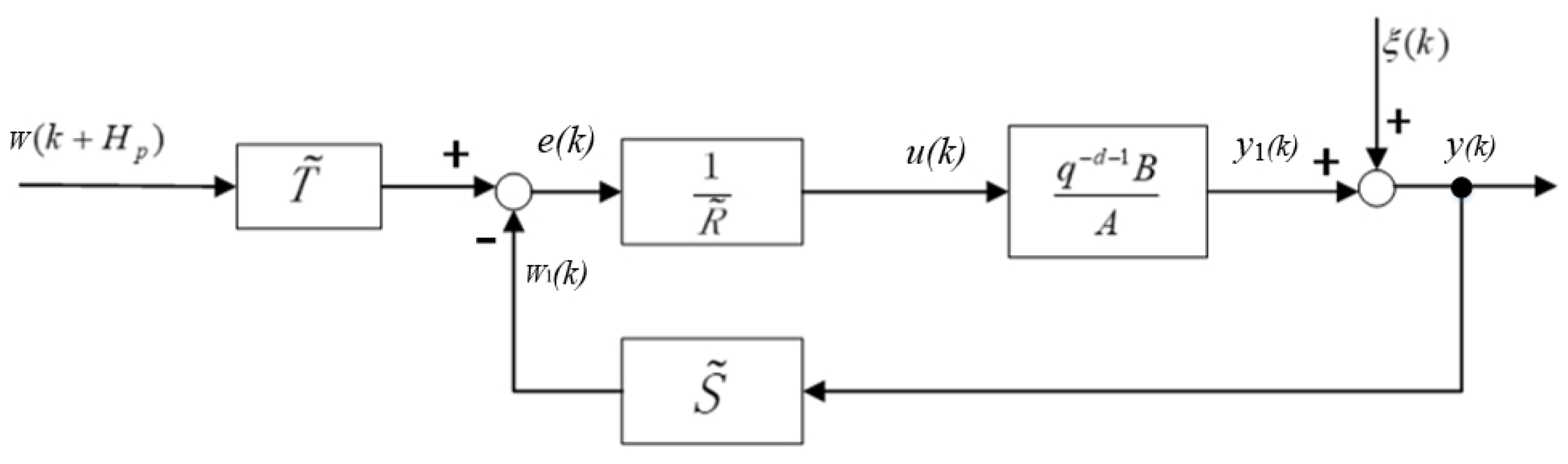
In this section, we will introduce the principle of MPC and simplify the design of MPC according to the FOPDT object to obtain a simplified MPC controller.

2.1. MPC Principle

Since MPC was proposed, there have been several influential classical algorithms. Each controller has different algorithm forms, has its own characteristics, and adapts to different application scenarios. The unified predictive control (UPC) proposed by Dutch scholar Soeterboek et al. is a general framework under SISO condition [8].

The prediction model is as follows:

$$y\left(k\right)={\displaystyle \frac{q^{-d}B\left(q^{-1}\right)}{A\left(q^{-1}\right)}}u\left(k-1\right)+{\displaystyle \frac{T\left(q^{-1}\right)}{D\left(q^{-1}\right)}}e\left(k\right),$$

(1)

where y(k) is the object output, u(k) is the control variable, e(k) denotes white noise, $A(q^{-1})=1+a_1{q}^{-1}+\cdots +a_n{q}^{-n_A}$, $B(q^{-1})=b_0+b_1{q}^{-1}+\cdots +b_{n_B}{q}^{-n_B}$, and d is the time delay. $\xi (k)={\displaystyle \frac{T(q^{-1})}{D(q^{-1})}}e(k)$ denotes the disturbance imposed on the output, $T(q^{-1})$ and $D(q^{-1})$ are polynomials with respect to $q^{-1}$.

The performance index is defined as follows:

$$J=\sum _{i=Hm}^{Hp}{[P\hat{y}(k+i)-P(1)w(k+i)]}^2+\rho \sum _{i=1}^{Hp-\hat{d}}{\left[{\displaystyle \frac{Q_n}{Q_{\mathrm{d}}}}u(k+i-1)\right]}^2,$$

(2)

and the constraint conditions are as follows:

$$\varphi Pu(k+i-1)=01\le H_c<i\le H_p-\hat{d},$$

(3)

where w(k) is the reference trajectory, $H_c$ is the control time domain, $H_m$ is the minimum cost time domain, $H_P$ is the prediction time domain. $\varphi$, $P(q^{-1})$ is a polynomial used to adjust the closed-loop servo performance, and $P(1)$ is the steady-state value of P. $Q_n(q^{-1})$ and $Q_d(q^{-1})$ constitute the filter of the controller output. $\phi (q^{-1})$ is a minimum polynomial of ${\phi }_w$ and ${\phi }_{\xi }$, where ${\phi }_w(q^{-1})w(k)=0$ and ${\phi }_{\xi }(q^{-1})\xi (k)=0$. Such a design is used to eliminate the steady-state error. $\rho$ is the weighting factor. This objective function also unifies the objective functions used by several main controllers [23].

The principle of the control system is shown in Figure 1 [8].

In Figure 1, the control law satisfies

$$\tilde{R}u(k)=-\tilde{S}y(k)+\tilde{T}w(k+H_p).$$

(4)

In Equation (4), $\tilde{R},\tilde{S},\tilde{T}$ are, respectively,

$$\tilde{R}=\hat{A}T{Q}_d+q^{-1}(H{Q}_d+\hat{A}T{Q}_d{V}_2+\rho \hat{A}TZ+\rho \hat{A}T{Q}_d{Z}_2),$$

(5)

$$\tilde{S}=\hat{A}F{Q}_d,$$

(6)

$$\tilde{T}=\hat{A}(q^{-1})P(1)T(q^{-1})Q_d(q^{-1})V(q^{-1}),$$

(7)

$\tilde{R},\tilde{S},\tilde{T},\hat{A},T,V_2,Z,Z_2,P$ is a polynomial of $q^{-1}$. The polynomial degrees of $\tilde{R},\tilde{S},\tilde{T}$ are $n_R,n_S,n_T$. The specific derivation process is quite complex (see [8] for details).

2.2. The Simple Design of MPC

The controlled object with self-balancing ability can be approximated as an FOPDT, and its transfer function is

$$G(s)={\displaystyle \frac{K}{\tau s+1}}{e}^{-{\tau }_{d}s},$$

(8)

where K is the static gain, $\tau$ is the time constant, and ${\tau }_d$ is the delay time. In the controller design process, these parameters are estimates, so use $\hat{K}$ instead of K, use $\hat{\tau }$ instead of $\tau$, and use ${\hat{\tau }}_d$ instead of ${\tau }_d$.

MPC, when used in computer control systems, needs to be discretized. In general, the sampling period is required to be ${\displaystyle \frac{1}{5}}$ to ${\displaystyle \frac{1}{15}}$ of the time constant of the object. The symbol $\theta$ is used to represent the ratio of the time constant to the sampling period: $\theta =\raisebox{1ex}{$\hat{\tau }$}\!\left/ \!\raisebox{-1ex}{$T_s$}\right.$. Suppose that $T_d$ is an integer multiple of sampling period $T_s$; that is, ${\hat{\tau }}_d=\hat{d}{T}_s$, $\hat{d}$ is an integer. Then, the discrete transfer function of the object is

$$\hat{G}(q^{-1})={\displaystyle \frac{b{q}^{-1}}{1-a{q}^{-1}}}{q}^{-d},$$

(9)

in (9), $a=e^{-\frac{1}{\theta }}, b=\hat{K}(1-a)$.

In the reference [8], according to the characteristics of most steady-state process objects, taking into account the requirements of rapidity, robustness and stability, it is recommended to select the parameters as shown in

Table 1. Parameter selection of the simple design.

Parameter	$\mathit{\varphi }$	P	T	$\hat{\mathit{D}}$	${\mathit{\xi }}_{det}$	$\mathit{\rho }$	${\mathit{H}}_{\mathit{m}}$	${\mathit{H}}_{\mathit{c}}$
values	$\Delta$	1	$\hat{A}(1-\mu q^{-1})$	$\hat{A}\Delta$	0	0	$\hat{d}+1$	1

.

According to the study in [13], Equations (5)–(7) are reduced to

$$\tilde{R}=T+q^{-1}H,$$

(10)

$$\tilde{S}=F,$$

(11)

$$\tilde{T}=TV(1),$$

(12)

in the equation

$$H={\mathbf{R}}_v^{-1}\sum _{i=1}^{H_l}{H}_i{G}_i(1),$$

(13)

$$F={\mathbf{R}}_v^{-1}\sum _{i=1}^{H_l}{F}_{i+d}{G}_i(1),$$

(14)

$$V={\mathbf{R}}_v^{-1}\sum _{i=1}^{H_l}{G}_i(1)q^{-(i-1)},$$

(15)

$${\mathbf{R}}_v=\sum _{i=1}^{H_l}{G}_i^2(1),$$

(16)

$$H_i=h_{i0}+h_{i1}{q}^{-1}+\cdots +{h_{i,n}}_H{q}^{-n_H},$$

(17)

$$F_i=f_{i0}+f_{i1}{q}^{-1}+\cdots +{f_{i,n}}_F{q}^{-n_F},$$

(18)

$$G_i=g_0+g_1{q}^{-1}+\cdots +g_{i-1}{q}^{-(i-1)},$$

(19)

$E_{i+d}$, $F_{i+d}$ are solved from the following Diophantine equation:

$${\displaystyle \frac{T}{\hat{D}}}=E_{i+d}+q^{-i+\hat{d}}{\displaystyle \frac{F_{i+d}}{\hat{D}}}i=1,2\cdots H_l,$$

(20)

$G_i$, $H_i$ are solved from the following Diophantine equation:

$${\displaystyle \frac{\hat{B}\hat{D}{E}_{i+d}}{T}}=G_i+q^{-i}{\displaystyle \frac{H_i}{T}}i=H_m-\hat{d},\cdots H_p-\hat{d}.$$

(21)

2.2.1. Solve $E_{i+d},F_{i+d},G_i,H_i$

Equation (20) is multiplied by $\hat{D}$ on both sides. From the principle of the equal coefficient of the $q^{-1}$ polynomial, the following equation can be derived:

$$E_{i+d}=1+(1-\mu )(q^{-1}+q^{-2}+\cdots +q^{-(i+\hat{d}-1)}),$$

(22)

$$F_{i+d}=(1-\mu )(1-a{q}^{-1}).$$

(23)

Equation (21) is multiplied by T on both sides. From the principle of the equal coefficient of the $q^{-1}$ polynomial, $g_i=\hat{K}{a}^i(1-a)$ can be derived; thus,

$$G_i=\hat{K}(1-a)(1+a{q}^{-1}+a^2{q}^{-2}+\cdots +a^{i-1}{q}^{-(i-1)}),$$

(24)

$$H_i=\hat{K}(1-a)(a^i(1-\mu q^{-1})+(1-\mu )q^{-d}).$$

(25)

2.2.2. Solve $\tilde{R},\tilde{S},\tilde{T}$

Equation (25) combined with (13) yields

$$\begin{array}{c}H={\mathbf{R}}_v^{-1}{\displaystyle \sum _{i=1}^{H_l}}{H}_i{G}_i(1)=\hfill \\ {\mathbf{R}}_v^{-1}{\displaystyle \sum _{i=1}^{H_l}}{a}^i{G}_i(1)\hat{K}(1-a)(1-\mu q^{-1})+{\mathbf{R}}_v^{-1}{\displaystyle \sum _{i=1}^{H_l}}{G}_i(1)\hat{K}(1-a)(1-\mu )q^{-\hat{d}}.\hfill \end{array}$$

(26)

Based on Equation (24), let q = 1; then,

$$G_i(1)=\hat{K}(1-a^i),$$

(27)

$$a^i=(1-G_i(1))/\hat{K}.$$

(28)

Let $\kappa$, $\eta$, $\alpha$ be forms (29)–(31)

$$\kappa =\hat{K}{{\mathbf{R}}_v}^{-1}\sum _{i=1}^{H_l}{G}_i(1)=\sum _{i=1}^{H_l}(1-a^i)/\sum _{i=1}^{H_l}{(1-a^i)}^2,$$

(29)

$$\eta =\kappa (1-a)(1-\mu ),$$

(30)

$$\alpha =\mu (1-\kappa (1-a)).$$

(31)

Equation (26) combined with (27)–(31) and (10) yields

$$H=(\kappa -1)(1-a)(1-\mu q^{-1})+\kappa (1-a)(1-\mu )q^{-\hat{d}},$$

(32)

$$\tilde{R}=T+q^{-1}H=1-(1+\alpha -\eta )q^{-1}+\alpha q^{-2}-\eta q^{-(\hat{d}+1)}.$$

(33)

Equation (11) combined with (23), (29) and (14) yields

$$\tilde{S}=F={\mathbf{R}}_v^{-1}\sum _{i=1}^{H_l}{F}_{i+d}{G}_i(1)=\kappa (1-\mu )(1-a{q}^{-1})/\hat{K},$$

(34)

$$V={\mathbf{R}}_v^{-1}\sum _{i=1}^{H_l}{G}_i(1)q^{-(i-1)}.$$

(35)

Equation (12) combined with (29) and (15) yields

$$\tilde{T}=TV(1)=\kappa (1-\mu q^{-1})(1-a{q}^{-1})/\hat{K}.$$

(36)

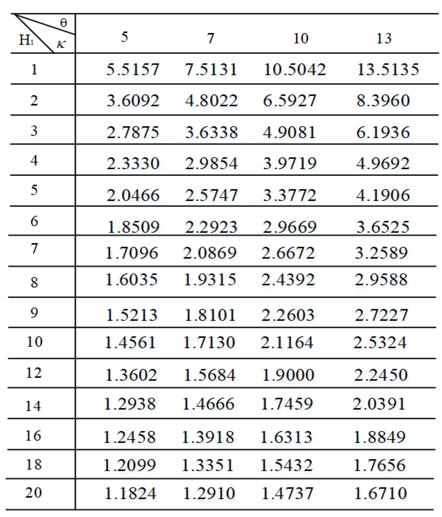
2.2.3. Calculation of κ Value

From Equations (33), (35) and (36), it can be seen that the relevant parameters $\eta$ and $\alpha$ of the controller are related to κ. From Equation (29), it can be seen that the κ value is related to $H_i$ and a, while a depends on the $\theta$ value. Therefore, the $\kappa$ value is only related to $H_i$ and $\theta$, and $a=e^{-\frac{1}{\theta }}$ is substituted into the Equation (29). The results of κ value are shown in Figure 2.

3. Characteristic Analysis of the Closed-Loop System

In the previous section, the controlled object is approximated as an FOPDT. The $\theta$ and $H_i$ are determined, and the $\kappa$ value is obtained. The $q^{-1}$ polynomials of $\tilde{R}$, $\tilde{S}$ and $\tilde{T}$ are obtained by substituting them into Equations (33), (35) and (36), respectively. It can be seen that the calculation of the control law is greatly simplified. Now, only simple arithmetic operations are needed, which are equivalent to the calculation of PID, and the method of determining parameters is more concise. Next, we will study the control performance of the controller.

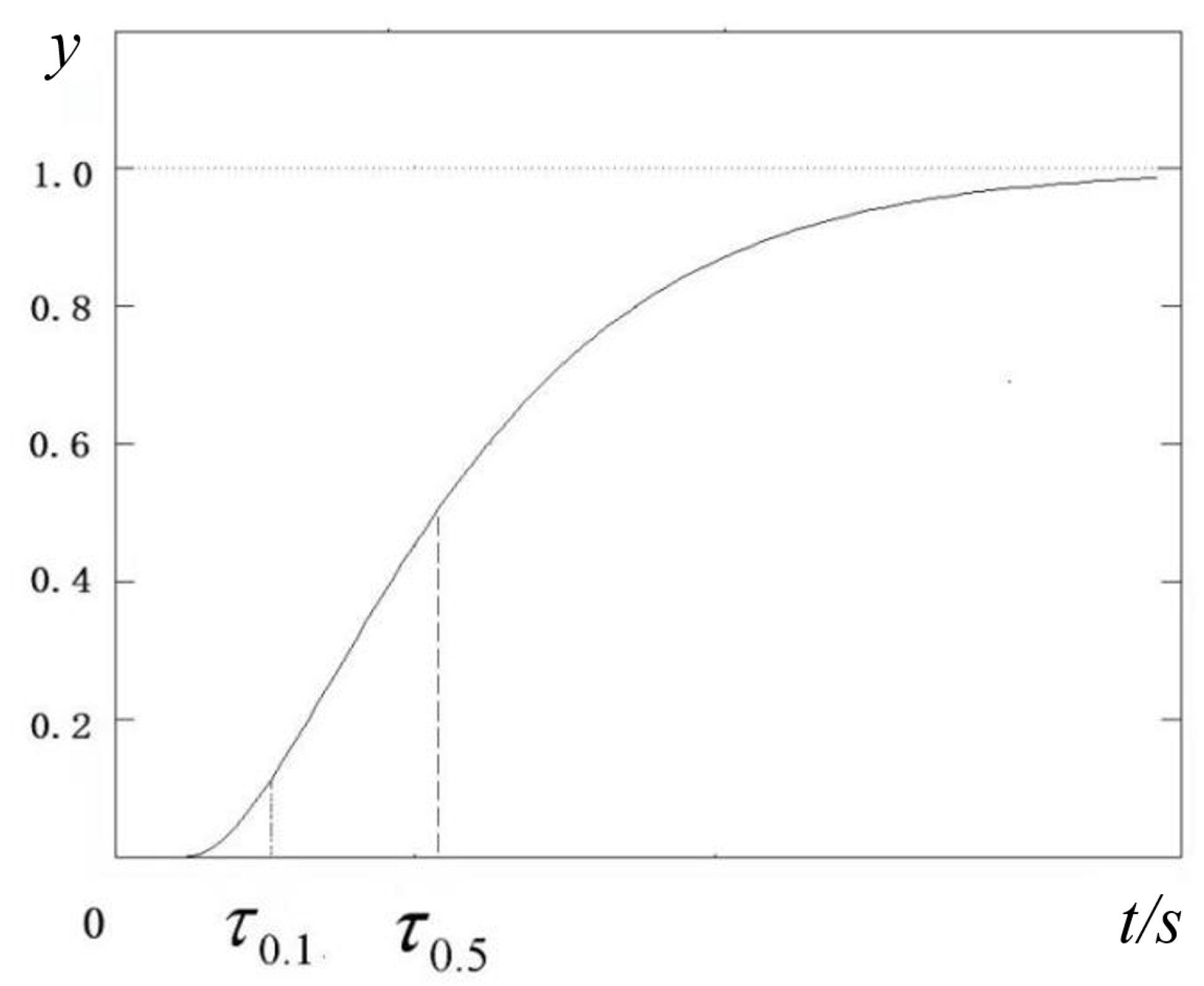
3.1. Ideal Dynamic Characteristics

When the model is accurate, it can be deduced from Figure 1 that the transfer function of the closed-loop system is

$$G_c(q^{-1})={\displaystyle \frac{q^{-(d+1)}B\tilde{T}}{A\tilde{R}+q^{-(d+1)}B\tilde{S}}}.$$

(37)

Let $\nu =1-\kappa (1-a)$, which can be simplified to

$$G_c(q^{-1})=q^{-(d+1)}{\displaystyle \frac{1-\nu }{1-\nu q^{-1}}}.$$

(38)

This is an FOPDT with a pole of $\nu$, a static gain of 1, and a constant delay time. Therefore, the following conclusions are drawn about the impact on the closed-loop system:

(1) When the value of $H_i$ is small enough to make $\kappa >{(1-a)}^{-1}$ (i.e., $\nu <0$), the closed-loop system will oscillate and diverge;

(2) When the value of $H_i$ makes $\kappa <{(1-a)}^{-1}$ (i.e., $\nu >0$), the closed-loop system is stable, and there exists the following relationship: $H_i$ increases = > $\kappa$ decreases = > $\nu$ increases = > system tracking speed slows down.

Therefore, although most of the parameters in the reduced design of UPC are fixed, the response speed of the closed-loop system can be adjusted by changing $H_i$. This choice is more concise than PID.

It can also be seen that when the model is accurate, the parameter $\mu$ has no effect on the transfer function of the closed-loop system. However, $\mu$ is of great significance for overcoming interference and robustness.

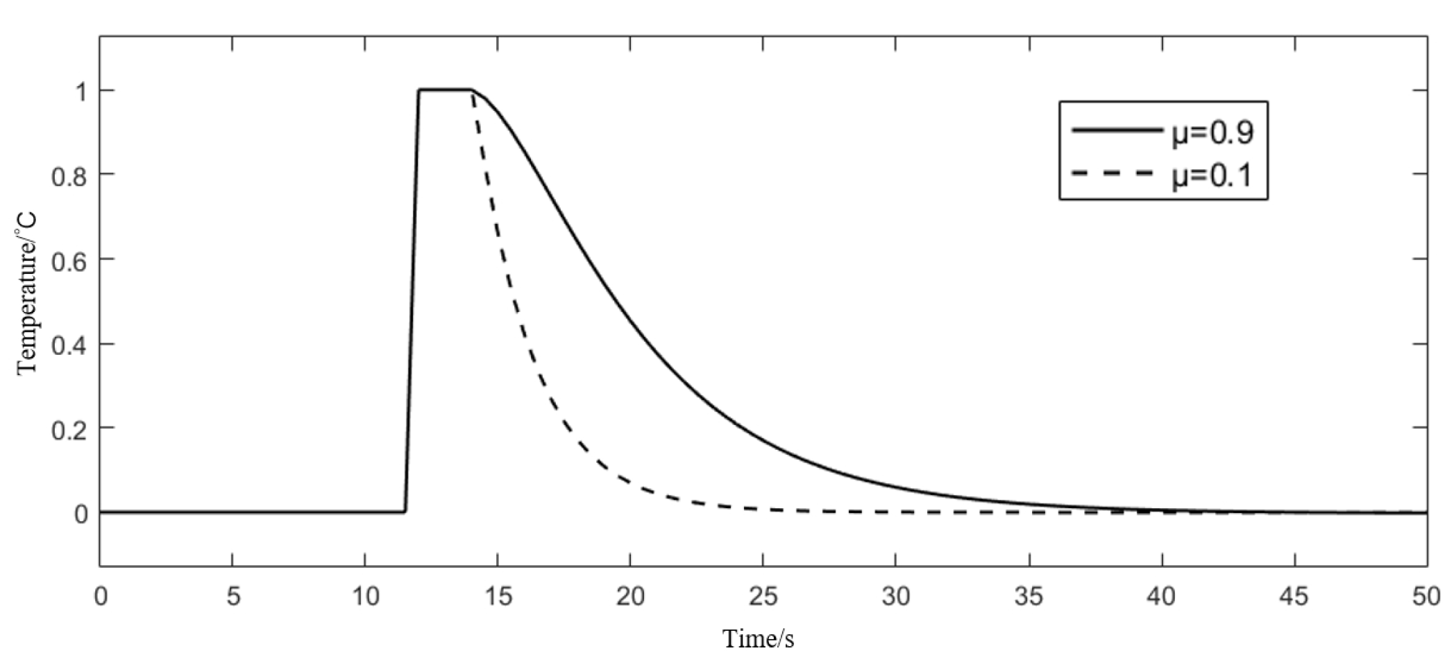
3.2. Interference Channel Characteristics

In this paper, the simulation method is used for analysis. Let the transfer function of the real object be $G(s)={\displaystyle \frac{1}{1+5s}}{e}^{-2s}.$

The static gain, time constant and delay time of the model are accurately obtained. Taking $T_s$ = 0.5 and $H_l$ = 10, the output is given a step interference with an amplitude of 1, and a different $\mu$ is taken, respectively. The Matlab simulation (MathWorks 2016a) results are shown in Figure 3 (solid line $\mu$ = 0.9, dashed line $\mu$ = 0.1).

It can be seen that the value of $\mu$ has an important influence on the response of the interference channel. The smaller the $\mu$ is, the more sensitive the system is, and the faster the disturbance can be overcome. However, the smaller the $\mu$ is, the lower the robustness of the system will be.

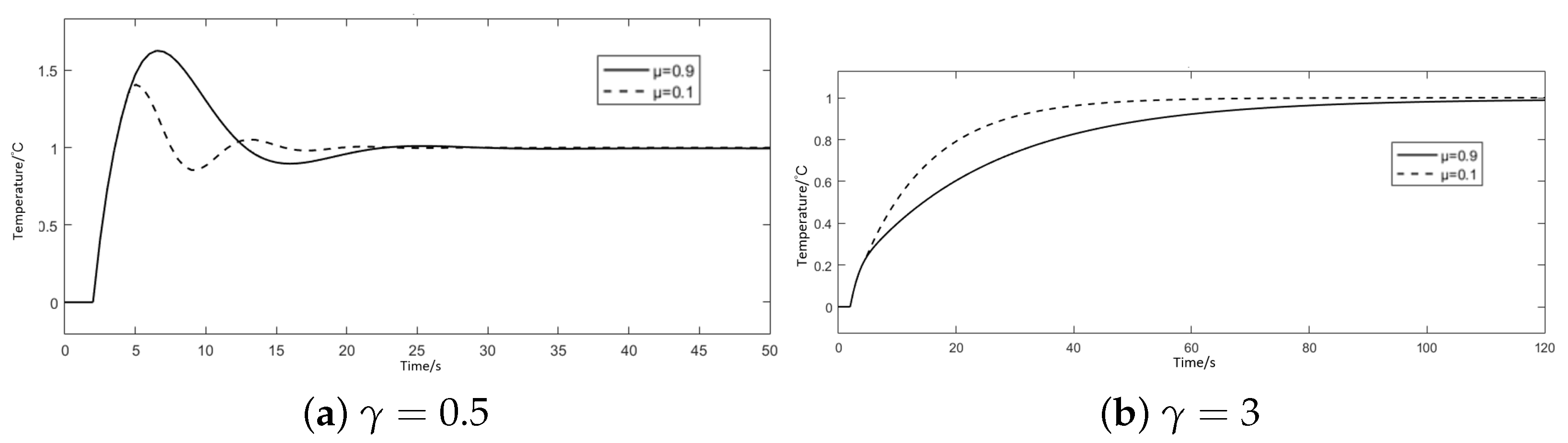
3.3. Robustness Analysis

The Matlab simulation results are compared and analyzed considering the aspects of static gain, time constant, delay time and high order object.

3.3.1. Static Gain Mismatch

The transfer function of the object is $G(s)={\displaystyle \frac{1}{1+5s}}{e}^{-2s}$.

The time constant and delay time of the model are accurate. Given the static gain $\hat{K}=\gamma K$, $T_s$ = 0.5, $H_l$ = 10, let $\gamma =0.5$ and $\gamma =3$, respectively. The simulation results are shown in Figure 4 (solid line $\mu$ = 0.9, dashed line $\mu$ = 0.1).

It can be seen that when the static gain estimation is too large, the closed-loop response becomes slower and the system is more stable. When the static gain estimation is too small, the system becomes unstable, and even significant oscillations are observed. Even if there is a gain error of 3 times, the choice of $\mu$ = 0.1 at the expense of robustness still does not exceed the stable boundary.

3.3.2. Mismatch of Time Constants

The static gain and delay time are set accurately, but the time constants are $\hat{\tau }/\tau =2$ and $\hat{\tau }/\tau =0.5$, respectively. Take, $T_S=0.1\hat{\tau }$, $H_l$ = 10. The simulation results are shown in Figure 5.

It can be seen that when the time constant estimation is too large, there are obvious overshoots and oscillations, and the stability margin is reduced. When the time constant estimation is too small, the stability margin of the transition process is large. The small value of $\mu$ can accelerate the reaction speed of the system, and there is a considerable margin from the stability boundary at the expense of robustness.

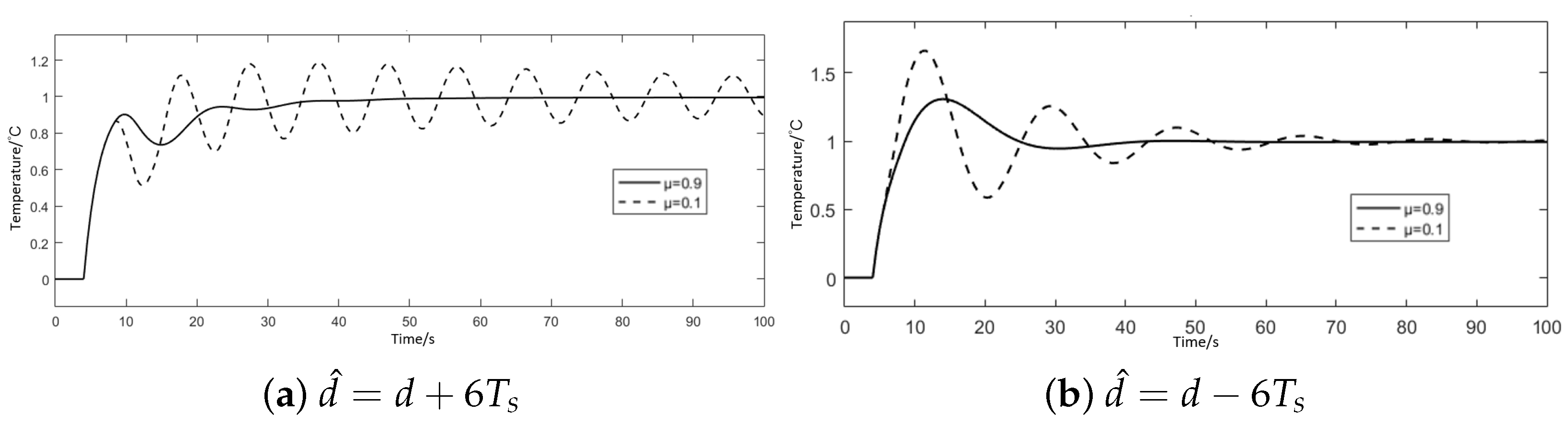
3.3.3. Delay Time Mismatch

The real transfer function of the phenomenon is $G(s)={\displaystyle \frac{1}{1+5s}}{e}^{-4s}$, and the static gain and time constant are accurate. Take $T_s$ = 0.5, $H_l$ = 10, and let $\hat{d}=d+6T_s$, $\hat{d}=d-6T_s$.

The simulation results are shown in Figure 6.

It can be seen that when the delay time is estimated too great, the system does not produce overshoot. When the delay time deviation is large and the $\mu$ value is small, the system tends to oscillate. In this case, reducing the large $\mu$ value can ensure the stability of the system and highlight the value of the $\mu$ value.

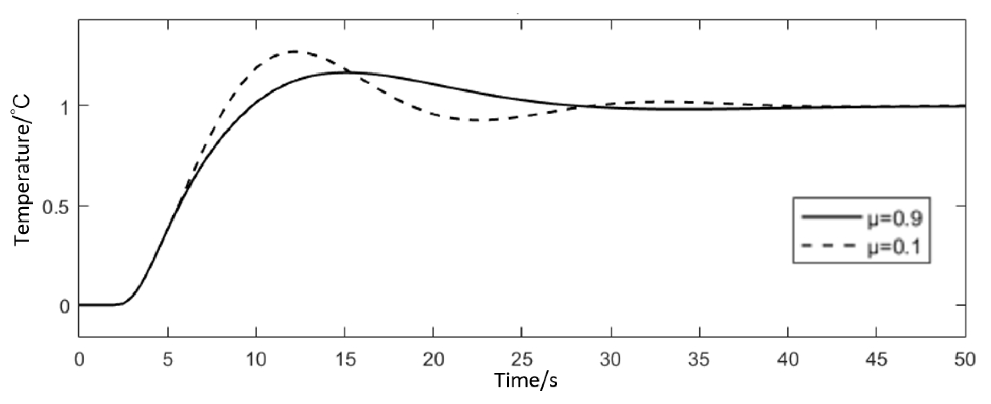
3.3.4. High-Order Object

Set the real object transfer function as $G(s)={\displaystyle \frac{1}{(1+5s){(1+s)}^2}}{e}^{-2s}$. Suppose that the static gain is accurate. Assume that the static gain is accurate, $\tau$ = 5, $T_s$ = 0.5, $H_l$ = 10.

The simulation results are shown in Figure 7.

It can be seen that the control effect of high-order objects is still good. When the value of $\mu$ is small, the system tends to oscillate and has a large overshoot. In fact, a better control effect can be obtained by adjusting the time constant and delay time.

3.4. Comparison with PID Control

In order to verify the effectiveness of the MPC simple design, the simulation system is built by MATLAB SIMULINK, and the control effects of the MPC simple design and the PID are compared and verified. The control object adopts the model of the study [6]: $G\left(s\right)={\displaystyle \frac{1}{(s+1)(0.1s+1)(0.01s+1)(0.001s+1)}}$.

The set value y (t) is given as Equation (39) to facilitate the observation of its control response curve.

$$y(t)=\left\{\begin{array}{c}1,\begin{array}{cc}& 0<t\le 5\end{array}\\ -1,\begin{array}{cc}& 5<t\le 10\end{array}\end{array}\right..$$

(39)

A step disturbance with a value of −0.5 is added at 6 s.

The PID parameter tuning method in [6] is used to set the sampling period $T_s$ = 0.01 s, and the control object is discretized. The gain $K_{180}$ and period $T_{180}$ of the −180° phase point are 0.0135 and 0.2003, the digital frequency ${\theta }_{180}$ (${\theta }_{180}$ = 2$\pi$$T_0$ / $T_{180}$) is 0.3136, ${\rho }_K$ and ${\rho }_T$ are 0.2989 and 0.7861, and the PID algorithm’s parameters $K_P$, $T_I$ and $T_D$ are

$$\begin{array}{c}{K}_P={\displaystyle \frac{{\rho }_K}{K_{180}}}=22.1407,\hfill \\ T_I={\displaystyle \frac{2\pi {\rho }_T{T}_0}{{\theta }_{180}}}=0.1574,\hfill \\ T_D={\displaystyle \frac{T_1}{4}}=0.0394.\hfill \end{array}$$

According to [6], the parameter tuning method is stronger than the method in [24]. This method obtains that the steady-state gain $K_0$ of the controlled object is 1, the gain $K_{180}$ and the period $T_{180}$ of the −180° phase point are 0.0091 and 0.199, and the PID algorithm’s parameters $K_P$, $T_I$ and $T_D$ are

$$\begin{array}{c}{K}_P={\displaystyle \frac{0.3-0.1{\lambda }^4}{K_{180}}}=32.8670,\hfill \\ T_I={\displaystyle \frac{0.6T_{180}}{1+2\lambda }}=0.1173,\hfill \\ T_D={\displaystyle \frac{0.15(1-\lambda )T_{180}}{1-0.95\lambda }}=0.0298,\hfill \\ \lambda =K_{180}/K_0.\hfill \end{array}$$

In this paper, the design of simplified MPC algorithms needs to add a pure delay object according to the first-order inertia. This object can be regarded as a series of four inertia links. Because the time constant is different by an order of magnitude, it is approximated as the slowest inertia link, and the control object is simplified into $G\left(s\right)={\displaystyle \frac{1}{(s+1)}}$.

According to the above simplified transfer function, the simplified MPC controller is designed. Take the sampling period $T_s$ = 0.1, $H_l$ = 5, and look up

Table 2. MPC function block input and output variables and description.

Variable Name	Explanation	In/Out
FB	feedback input	In
SP	set value	In
Gain	Static gain of controlled object	In/out
Time constant	Time constant, unit: seconds, range 10 to 65,535	In/out
Time delay	Delay time, unit: seconds, range 0 to Time constant	In/out
Update	Parameter identification command: 0 not identified, 1 identified Gain, 2 identified Time constant and Time delay	In
Status	Identify process state markers. When Update = 1 or 2, Status = 5 means waiting to rewrite the SP value to continue the identification process; status = 6 indicates that the identification is over and the parameters have been refreshed.	out
Output exec	Actuator actual execution value feedback	In
Output	Output of the controller	out

to obtain κ = 3.3772. Then let $\mu$ = 0.1 (the value range of $\mu$ be (0–1); the greater the $\mu$ is, the stronger the robustness is, but the rapidity is poor. The simulation does not require high robustness, so take 0.1), a = $e^{-1/10}$ = 0.9048. This yields

$$\begin{array}{c}\eta =\kappa (1-a)(1-\mu )=0.2894,\hfill \\ \alpha =\mu (1-\kappa (1-a))=0.06785,\hfill \\ R=1-(1+\alpha -\eta )q^{-1}+\alpha q^{-2}-\eta q^{-\hat{\mathrm{d}}+1}=1-0.7785q^{-1}-0.2216q^{-2},\hfill \\ S=\kappa (1-\mu )(1-a{q}^{-1})=3.3095-2.75q^{-1},\hfill \\ T=\kappa (1-a{q}^{-1})(1-\mu q^{-1})=3.3772-3.3934q^{-1}+0.3056q^{-2}.\hfill \end{array}$$

If the adjustment time of the simplified MPC is shortened, the $H_l$ is reduced, but according to the previous discussion, the reduction of $H_l$ may be an overshoot or even divergence. Take the sampling period $T_s$ = 0.1, $H_l$ = 2 and look up Table 2 to obtain $\kappa$ = 6.5927. Then, let $\mu$ = 0.1, a = $e^{-1/10}$ = 0.9048. This yields

$$\begin{array}{c}\eta =\kappa (1-a)(1-\mu )=0.5649,\hfill \\ \alpha =\mu (1-\kappa (1-a))=0.0372,\hfill \\ R=1-(1+\alpha -\eta )q^{-1}+\alpha q^{-2}-\eta q^{-\hat{\mathrm{d}}+1}=1-0.4724q^{-1}-0.5276q^{-2},\hfill \\ S=\kappa (1-\mu )(1-a{q}^{-1})=5.9334-5.3686q^{-1},\hfill \\ T=\kappa (1-a{q}^{-1})(1-\mu q^{-1})=6.5927-6.6243q^{-1}+0.5965q^{-2}.\hfill \end{array}$$

The Simulink simulation control system is built as shown in Figure 8.

The output response curve of the controlled object of the PID control and the simplified MPC control, using the PID parameter tuning method presented in [5], is shown in Figure 9.

From the simulation results shown in Figure 9, we can see that the simplified MPC control has no overshoot and the PID control has a 36.1% overshoot, which means that the control process is more stable than the PID control. The absence of the oscillation process will not destroy the system, cause energy loss or even physical damage, and will not lead to problems such as quality degradation and production efficiency decline. It is more suitable for use in industrial processes. In terms of adjustment time, the two control effects are close, and the adjustment time is 0.7 s and 0.65 s, respectively. To increase the adjustment speed of the simplified MPC control, a smaller Hl can be selected, but this will affect the system. Therefore, in the actual industrial process application, it is recommended to use the $\kappa$ value where $H_l$ and $\theta$ are both 10, as in Table 2. At this time, the controller has good control performance and strong robustness; even if the object characteristics change, the controller effect is still good.

4. Simplify the Field Application of MPC Controller

In this section, we test the control effect of the simplified MPC controller based on the temperature and humidity control project of the air conditioning unit in a pharmaceutical laboratory.

4.1. Parameter Selection

In order to save the resources of the field controller and facilitate the use of engineering and technical personnel, the controller parameters are further simplified. The fixed selection takes the sampling interval $T_{\mathrm{s}}=\hat{\tau }/10$, then $a=e^{-\frac{1}{10}}$ is fixed. Considering the robustness and rapidity, $H_l=10$, $\mu =0.1$ are fixed, and $\kappa =2.1164$ is obtained by looking up the table, so

$$\tilde{R}=1-0.8985q^{-1}+0.07985q^{-2}-0.1814q^{-(\hat{d}+1)},$$

$$\tilde{S}=(1.9053-1.7239q^{-1})/\hat{K},$$

$$\tilde{T}=(2.117-2.1272q^{-1}+0.1915q^{-2})/\hat{K},$$

that is,

$$\begin{array}{c}u(k)=0.8985u(k-1)-0.07985u(k-2)\hfill \\ +0.1814u(k-(\hat{d}+1))+(1.9053y(k)-1.7239y(k-1))/\hat{K}\hfill \\ +(2.117w(k)-2.1272w(k-1)+0.1915w(k-2))/\hat{K}.\hfill \end{array}$$

The calculation amount of the simplified MPC control is equivalent to the calculation amount of the PID control, and the operation can be performed directly by the field controller.

4.2. Parameter Identification

Open-loop identification is simpler. However, the open loop is in an abnormal working state, the project may not be allowed, and its time is long, while the closed loop is in a normal working state, and its speed is slow. Therefore, this paper focuses on the method of closed-loop identification.

Due to the need to determine three object parameters, a closed-loop parameter identification method is proposed to identify static gain, time constant and delay time.

1. The identification of static gain needs to record two equilibrium points. The so-called equilibrium point is a stable state, and its control quantity does not change or changes very little. If the difference between the maximum and minimum values of u is less than a certain value within 20 $T_{\mathrm{s}}$ times, such as 0.05, the object is judged to enter the equilibrium state. If the criterion is not satisfied, the criterion of 20 $T_{\mathrm{s}}$ is performed again. The average value of u and y in this period is calculated as an equilibrium point $(u_1,y_1)$. By changing the setting value, the second equilibrium point $(u_2,y_2)$ is obtained by the same method, and the static gain $\hat{K}=(y_2-y_1)/(u_2-u_1)$ can be estimated.

2. The identification of time constant/delay time requires a transition process. Firstly, the object is judged to enter the equilibrium point according to the above method, and then the set value is changed, and the object enters the closed-loop transition process.

When the model is accurate, the delay time of the closed-loop system remains unchanged, and the pole is $\nu =1-\kappa (1-a)$. When the values of $\theta$ and $H_l$ are constant, the time constant of the closed-loop system is also fixed. Let $\theta$ = 10, $H_l$ = 10, $\nu$ = 0.7985, and the closed-loop time constant be ${\tau }_{\mathrm{c}}=0.44\tau$. Conversely, the original time constant $\tau =2.27{\tau }_c$ can be derived from the closed-loop time constant.

Ideally, the time constant should be the time when the amplitude changes by 63%, but the curve at 63% is not as steep as that at 50%, and the time point is more accurate at 50%. Assume that the setting value is changed to ${\Delta }_w$, the time when the feedback value changes 0.1 ${\Delta }_w$ is recorded as ${\tau }_{0.1}$, and the time when the feedback value changes 0.5 ${\Delta }_w$ is recorded as ${\tau }_{0.5}$, as shown in Figure 10. However, ${\tau }_{0.63}$ (i.e., ${\tau }_c$) is replaced by ${\tau }_{0.5}$, and the multiple is appropriately adjusted to 2.5, i.e., $\hat{\tau }\approx 2.5{\tau }_{0.5}$.

In theory, the delay time should be the time when the feedback value changes after the control quantity changes. However, due to the existence of noise, it is difficult to define the threshold of ‘change’. In this paper, the change of 10% amplitude time is used as a reference in the project, multiplied by a coefficient of 0.75.

The identified parameters are as follows:

$${\hat{\tau }}_d=0.75{\tau }_{0.1},$$

$$\hat{\tau }=2.5({\tau }_{0.5}-{\hat{\tau }}_d).$$

The closed-loop identification of time constant and delay time usually requires multiple iterations, as shown in Figure 11. In the iteration process, first of all, in order to have better robustness, a larger $\mu$ value is taken, and $\mu$ = 0.9. After repeated iterations, the identification is confirmed to be accurate, and then $\mu$ = 0.1 is changed to improve the response speed to interference.

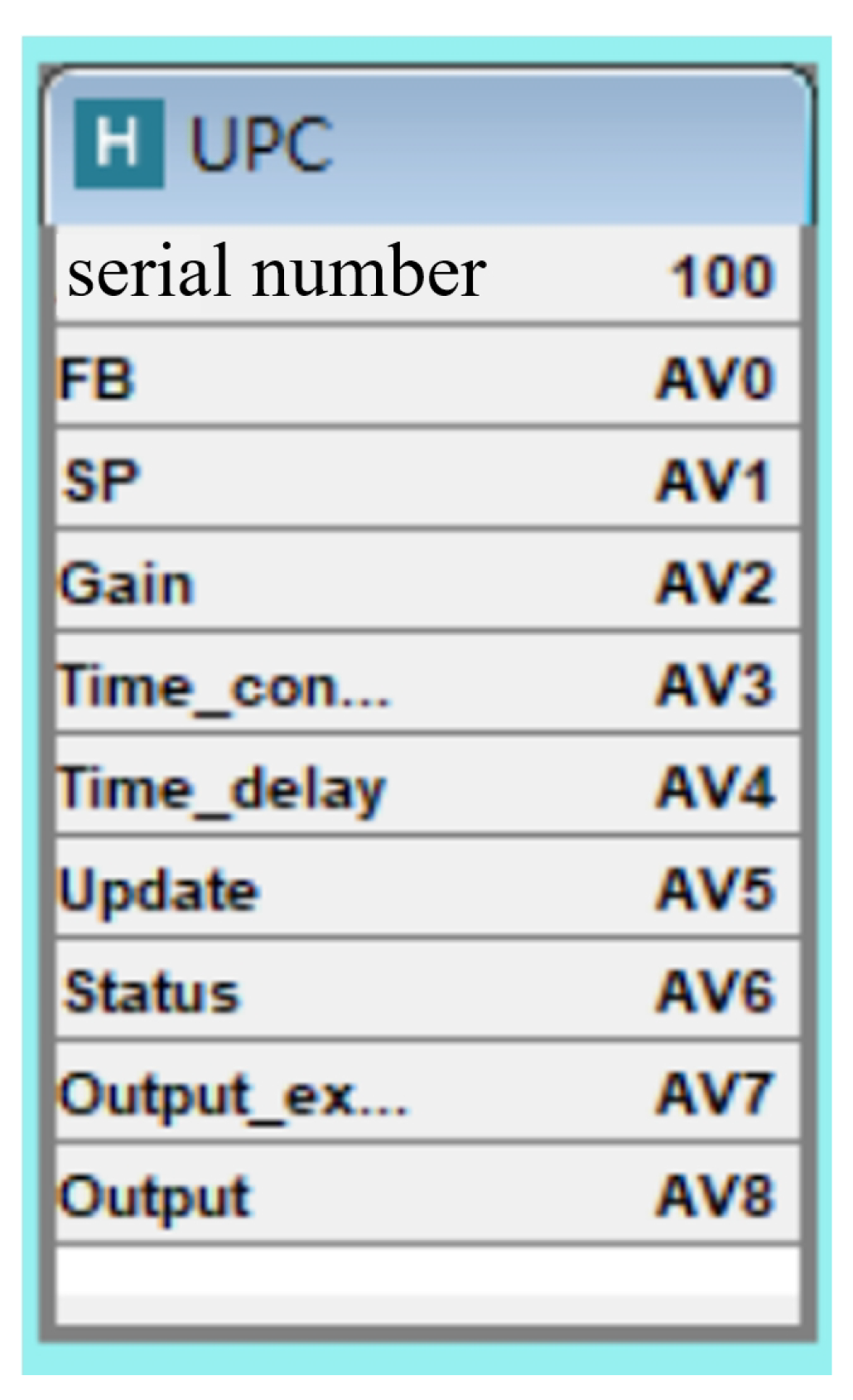
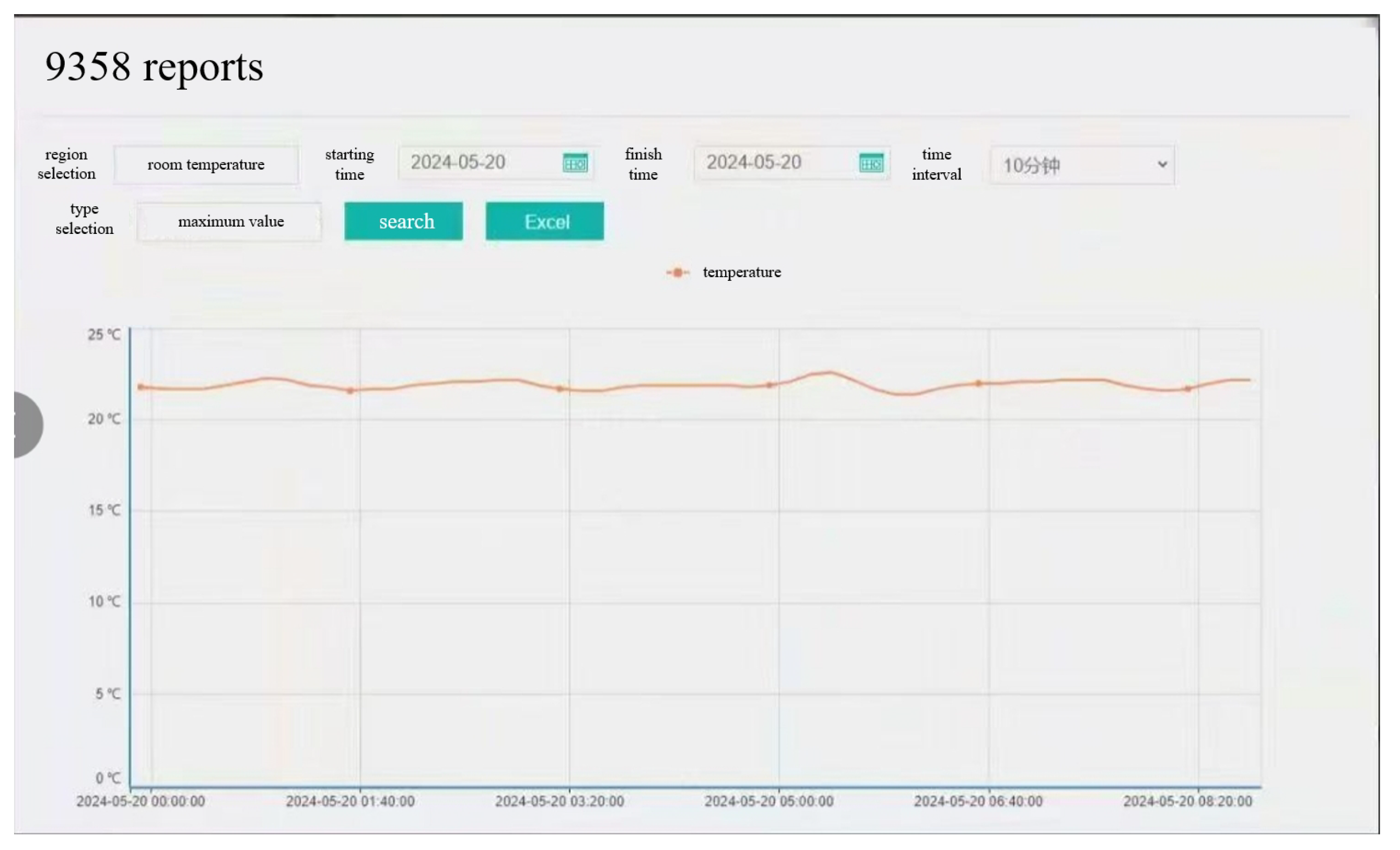
4.3. Design and Field Application of the MPC Function Block

The simplified MPC control algorithm, together with the parameter identification function, is encapsulated into a standard function block in the programmable controller (Manufacture: Beijing Hysine Yunda Technology Co., Ltd. Type: BLC series. Programming language: Hysine function block programming. Period for operating scan: 10 ms. Samping period: 10 ms. Communitcation protocol: BACnet.), as shown in Figure 12, and all input and output variables and parameters are shown in Table 2.

A drug laboratory used mice to test the effect of drugs. In order to ensure the comfort of the mice, the air conditioning unit was used to control the temperature and humidity of the room. The fresh air and return air are mixed together. If the humidity is too high, the cold water valve is used to dehumidify first, and the reheat valve is used to control the room temperature. For the temperature control loop, the temperature and humidity of the external air and the action of the cold water valve are regarded as the disturbance of the temperature control. The structure of the air conditioning unit is shown in Figure 13. Under this condition, the static gain identified by the MPC function block is 0.45, the time constant is 360 s, the delay time is 35 s, and the temperature is set to 22 °C. The obtained temperature response curve is shown in Figure 14.

It can be seen from the curve that the actual temperature fluctuation range is $\pm 0.7$ °C, which fully meets the requirements of users.

5. Conclusions

Predictive control is currently used in MIMO systems and has good control quality, but it has the problems of a large amount of computation, difficult parameter setting and difficult on-site maintenance. For the SISO process, the simplified MPC control law is formed by approximating the process object and simplifying the controller parameters. The algorithm only needs to identify the static gain, time constant and delay time of the object to enable its implementation. The calculation amount is small and is suitable for embedding the field controller. From the comparative simulation experiment, it can be seen that the simplified MPC control effect is obviously better than the PID control. The predictive control module of the programmable controller is developed to achieve the online identification of process objects and the simplified MPC control. The industrialization prospects of the MPC parsimony control replacing the PID algorithm are proved considering the aspects of control quality, convenience of parameter tuning, and the realization of the control algorithm.

References

1. Guo, L. Feedback and uncertainty: Some basic problems and results. Annu. Rev. Control 2020, 49, 27–36. [Google Scholar] [CrossRef]
2. Samad, T. A survey on industry impact and challenges thereof [Technical Activities]. IEEE Control Syst. Mag. 2017, 37, 17–18. [Google Scholar]
3. Shukla, M.K.; Rajput, K.; Yadav, A.K.; Prakash, S.A. Classical Techniques for PID Tuning. Int. Res. J. Eng. Technol. 2022, 9, 3440–3444. [Google Scholar]
4. Nie, Z.Y.; Li, Z.Y.; Wang, Q.G. A unifying Ziegler-nichols tuning method based on active disturbance rejection. Int. J. Robust Nonlinear 2022, 32, 9525–9541. [Google Scholar] [CrossRef]
5. Bazanella, A.S.; Pereira, L.F.A. A new method for PID tuning including plants without ultimate frequency. IEEE Trans. Control Syst. 2017, 25, 637–644. [Google Scholar] [CrossRef]
6. Liu, N.; Chai, T.Y.; Parraga, A. An Optimal Tuning Method of PID Controller Parameters. Acta Autom. Sin. 2023, 49, 2272–2285. [Google Scholar]
7. Schwenzer, M.; Ay, M.; Bergs, T. Review on model predictive control: An engineering perspective. Int. J. Adv. Manuf. Technol. 2021, 117, 1327–1349. [Google Scholar] [CrossRef]
8. Soeterboek, A.R.M. Predictive Control: A unified Approach; Prentice Hall: London, UK, 1992. [Google Scholar]
9. Soeterboek, A.; Verbruggen, H.; van den Bosch, P. On the Design of the Unified Predictive Controller. IFAC Proc. Vol. 1991, 24, 351–356. [Google Scholar] [CrossRef]
10. Wei, D.; Jiao, H.Y.; Feng, H.D. Nonlinear predictive control of refrigeration station system based on load forecasting. Control Theory Appl. 2021, 38, 1619–1630. [Google Scholar]
11. Feng, X.Y.; Wang, B.; Yang, C.L. Anti-disturbance predictive control of superheated steam temperature system for APS. Comput. Simul. 2022, 39, 141–145. [Google Scholar]
12. Zhu, Q.G.; Zhen, W.J.; Shi, J.K. Main steam pressure control method of 1000 MW unit based on state feedback-predictive control. Steam Turbine Technol. 2022, 64, 63–66. [Google Scholar]
13. Yao, Y.; Shekhar, D. State of the art review on model predictive control (MPC) in Heating Ventilation and Air-conditioning (HVAC) field. Build. Environ. 2021, 200, 107952.1–107952.18. [Google Scholar] [CrossRef]
14. Juneja, P.K.; Sunori, S.K.; Sharma, A.; Sharma, A.; Kumar, P.; Joshi, V.; Raizada, R. Comparison of closed loop performance of consistency process dynamics for various PID controller algorithms. J. Phys. Conf. Ser. 2021, 2070, 012113. [Google Scholar] [CrossRef]
15. da Silva, L.R.; Flesch, R.C.C.; Normey-Rico, J.E. Controlling industrial dead-time systems: When to use a PID or an advanced controller. ISA Trans. 2020, 99, 339–350. [Google Scholar] [CrossRef] [PubMed]
16. Maurya, S.; Peddoju, S.K.; Ahmad, B.; Chihi, I. (Eds.) Cyber Technologies and Emerging Sciences; Lecture Notes in Networks and Systems; Springer: Singapore, 2023; Volume 467. [Google Scholar]
17. Muresan, C.I.; Ionescu, C.M. Generalization of the FOPDT Model for Identification and Control Purposes. Processes 2020, 8, 682. [Google Scholar] [CrossRef]
18. Bi, J.; Tan, W.; Yu, M. Tuning of PID controllers for unstable first-order plus dead time systems. Chem. Prod. Process Model. 2023, 18, 877–891. [Google Scholar] [CrossRef]
19. Sha’aban, Y.A.; Lennox, B.; Laurí, D. PID versus MPC Performance for SISO Dead-time Dominant Processes. IFAC Proc. Vol. 2013, 46, 241–246. [Google Scholar] [CrossRef]
20. Ali, E.J.; Feki, E.; Mami, A. Dynamic Matrix Control DMC using the Tuning Procedure based on First Order Plus Dead Time for Infant-Incubator. Int. J. Adv. Comput. Sci. Appl. 2019, 10, 358–367. [Google Scholar] [CrossRef]
21. Lin, S.-K.; Lee, A.-C. Adaptive unified predictive control applied to first-order-plus-dead-time processes to eliminate unknown class of deterministic disturbance. Evol. Syst. 2012, 3, 45–56. [Google Scholar] [CrossRef]
22. Cordero, R.; Gonzales, J.; Estrabis, T.; Galotto, L.; Padilla, R.; Onofre, J. Variable Frequency Resonant Controller Based on Generalized Predictive Control for Biased-Sinusoidal Reference Tracking and Multi-Layer Perceptron. Energies 2024, 17, 2801. [Google Scholar] [CrossRef]
23. Zhang, Q. Research on Unified Predictive Control and Its Application in Thermal Process. Ph.D. Thesis, Tsinghua University, Beijing, China, 1998. [Google Scholar]
24. Åström, K.J.; Hägglund, T. Advanced PID Control; ISA: Pittsburgh, PA, USA, 2006. [Google Scholar]
Figure 1. Control system block diagram.
Actuators 14 00191 g001
Figure 2. The calculation results of κ value.
Actuators 14 00191 g002
Figure 3. Response of the step input of the interference channel.
Actuators 14 00191 g003
Figure 4. Static gain mismatch.
Actuators 14 00191 g004
Figure 5. Mismatch of time constant.
Actuators 14 00191 g005
Figure 6. Delay time mismatch.
Actuators 14 00191 g006
Figure 7. High-order objects.
Actuators 14 00191 g007
Figure 8. Simulink simulation of the simple design of the MPC control system.
Actuators 14 00191 g008
Figure 9. Simple MPC control output curve and PID control comparison chart [5,6].
Actuators 14 00191 g009
Figure 10. Positions of closed-loop step response τ 0.1 and τ 0.5 .
Actuators 14 00191 g010
Figure 11. The identification iterative process of time constant and delay time.
Actuators 14 00191 g011
Figure 12. MPC function block in field controller.
Actuators 14 00191 g012
Figure 13. Air conditioning unit temperature and humidity control.
Actuators 14 00191 g013
Figure 14. The actual control temperature curve of the MPC controller at the project site.
Actuators 14 00191 g014