High-Precision Control of Control Moment Gyroscope Gimbal Servo Systems via a Proportional–Integral–Resonant Controller and Noise Reduction Extended Disturbance Observer

Abstract

Speed control accuracy of gimbal servo systems for control moment gyroscopes (CMGs) is crucial for spacecraft attitude control. However, multiple disturbances from internal and external factors severely degrade the speed control accuracy of gimbal servo systems. To suppress the effects of these complex disturbances on speed control accuracy, a control method based on a proportional–integral–resonant (PIR) controller and a noise reduction extended disturbance observer (NREDO) is proposed in this paper. First, the disturbance dynamic model of an $(n+1)$th-order NREDO is derived. The integral of the virtual measurement of the lumped disturbance is an augmented state in the model. NREDO states are updated by using the estimation error of the augmented state. The NREDO significantly enhances the measurement noise suppression performance compared with an EDO. Second, a resonant controller is introduced to suppress the high-frequency rotor dynamic imbalance torque. The PIR controller is composed of a resonant controller in parallel with a PI controller. Numerical simulation and experimental results demonstrate the effectiveness of the proposed method.

1. Introduction

High-precision control of gimbal servo systems is one of the core and critical issues in control moment gyroscopes (CMGs) [1]. However, the gimbal servo system is severely affected by multiple disturbances from both internal and external factors, such as friction torque, cogging torque, gyroscopic torque caused by spacecraft motion, and rotor dynamic imbalance torque [2]. From the perspective of disturbance frequency, multiple disturbances can be classified into low-frequency disturbances and high-frequency disturbances. The low-frequency disturbances are related to gimbal angular speed, gimbal angular position, and spacecraft angular speed. The high-frequency disturbances are related to rotor angular speed [3]. Complex multiple disturbances will degrade the speed control accuracy of gimbal servo systems, and even affect the stability of the system. Therefore, it is crucial to suppress multiple disturbances to improve the speed control accuracy of gimbal servo systems.

To suppress the influence of the aforementioned disturbances, researchers have carried out extensive studies on a range of methods, including proportional–integral–derivative (PID) control [4,5,6,7], robust control [8,9,10], adaptive control [11,12,13,14], and sliding mode control [15,16,17]. Although feedback control methods can directly suppress multiple disturbances, their performance remains limited due to inadequate utilization of prior knowledge about disturbance characteristics. To enhance the disturbance suppression performance of feedback control methods, a resonant controller can be introduced into the control forward path. The resonant controller provides infinite open-loop gain at the resonant frequency, effectively suppressing specific frequency harmonic disturbances [18]. To suppress the 6th- and 12th-order harmonics on the d-axis and q-axis, two resonant controllers of corresponding frequencies are connected in parallel with a conventional PI controller. Additionally, resonant controllers are introduced into the speed controller to suppress harmonics caused by current measurement errors and cogging torque. Based on the proposed cascade scheme, speed fluctuations of permanent magnet synchronous motors (PMSMs) are obviously reduced [19]. The improved resonant controller can reduce the effects of sinusoidal voltage disturbances on steady-state currents. Moreover, the step response of the q-axis current exhibits better dynamic performance [20]. In [21], conventional resonant controllers have a fixed resonant frequency, making them suitable for periodic disturbances with a known frequency. Actually, the frequencies of disturbances in servo systems are uncertain. To address this, the resonant frequency is obtained by using a frequency estimation method. Thus, a PIR controller can be utilized to suppress high-frequency rotor dynamic imbalance torque. However, a PIR controller has limited performance with regard to suppressing other low-frequency disturbances, making it difficult to achieve high precision and stability in gimbal servo systems.

For other low-frequency disturbances, disturbance observers provide another feasible approach. Conventional disturbance observers have relatively low orders and large model errors, making them unable to accurately estimate complex disturbances. The extended disturbance observer (EDO) approximates complex disturbances by utilizing high-order time series or polynomial models [22]. Based on more accurate disturbance models, the estimation accuracy of complex multiple disturbances is significantly improved. To improve the estimation accuracy of flexible vibration, ref. [23] adopts a high-order polynomial to approximate disturbances in attitude dynamics of flexible spacecrafts. Notably, in order to improve disturbance estimation accuracy, an EDO usually needs to have a relatively high bandwidth. However, a high bandwidth makes it more sensitive to measurement noises, decreasing disturbance estimation accuracy. To address this, an attitude controller based on a noise reduction EDO (NREDO) has been utilized to improve the attitude control accuracy of flexible spacecraft [24]. Furthermore, the NREDO has already been applied to the issue of precise landing of quadrotors on moving platforms. The quadrotor landing experiment demonstrated that high-frequency noises in the output of observers were significantly reduced [25].

To further suppress complex multiple disturbances, a PIR-NREDO is designed for the CMG gimbal servo system, directly driven by a PMSM, in this paper. The main contributions of this paper are listed as follows.

(1)

To address multiple disturbances affecting gimbal servo systems, this paper classifies the disturbances into high-frequency periodic disturbance caused by rotor dynamic imbalance and other low-frequency disturbances based on frequency characteristics.

(2)

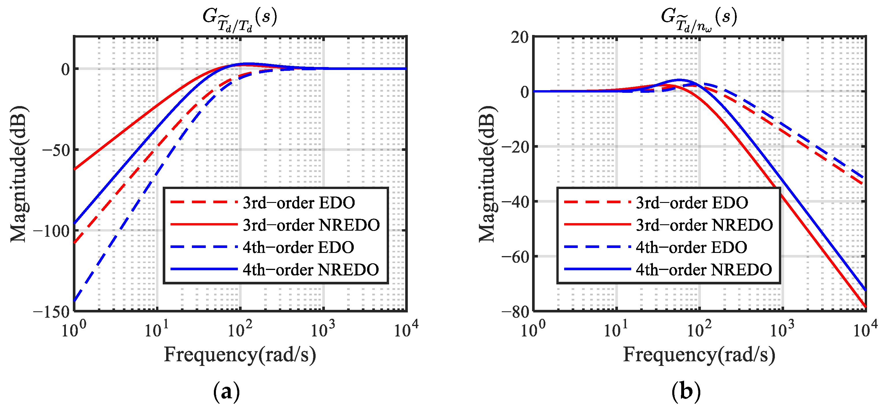
To minimize the disturbance estimation error caused by measurement noises, the integral of the virtual measurement of the lumped disturbance is derived to establish the disturbance dynamic model. Subsequently, an NREDO is designed based on the model. Innovatively, the estimation error of the augmented state is utilized to drive the convergence of NREDO error dynamics, thereby enhancing the suppression of measurement noise.

(3)

A resonant controller is utilized to reject rotor dynamic imbalance disturbance, instead of using a disturbance observer to estimate it. The composite speed controller is composed of a PIR controller and an NREDO. The proposed control scheme can maximize the suppression of complex disturbances, improving the speed control accuracy of gimbal servo systems.

The rest of this paper is organized as follows: A mathematical model of the gimbal servo system and an analysis of multiple disturbances are presented in Section 2. The PIR-NREDO is proposed in Section 3. Simulation and experimental results are presented in Section 4 and Section 5, respectively. The conclusion is given in Section 6.

2. Mathematical Model and Problem Statement

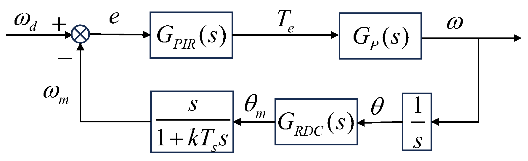
2.1. Mathematical Model of Gimbal Servo System

The gimbal servo system is directly driven by a PMSM, and the mechanical motion equation of the PMSM is given by the following [26]:

$$J\dot{\omega }+D\omega =T_e-T_d$$

(1)

where $T_e$ is the electromagnetic torque; $J$ is the moment of inertia; $D$ is the damping coefficient; $\omega$ is the mechanical angular speed of the gimbal motor; $T_d$ is the equivalent disturbance torque acting on the gimbal axis; and $T_d$ represents the sum of multiple disturbance torques, such as friction torque $T_f$, cogging torque $T_{cog}$, gyroscopic torque caused by spacecraft motion, rotor dynamic imbalance torque $T_r$, and the equivalent disturbance introduced by model inaccuracies, denoted by $T_u$.

Assumption 1.

The lumped disturbance $T_d$ is continuous and has bounded derivatives, i.e., $‖T_d^{\left(j\right)}‖\le \gamma$, $j=\mathrm{1,2},\dots ,n$, $n>0$, where $\gamma$   is a positive constant.

The electromagnetic torque equation of the PMSM can be written as follows [26]:

$$T_e=1.5p[{\psi }_f{i}_q+(L_d-L_q\left)i_d{i}_q\right]$$

(2)

where $i_d$ and $i_q$ are the d-axis and q-axis stator currents; $L_d$ and $L_q$ are the d-axis and q-axis stator inductances; $p$ is the number of pole pairs; and ${\psi }_f$ is the stator flux linkage.

This paper utilizes a surface-mounted PMSM, i.e., $L_d=L_q$, so (2) can be simplified as follows:

$$T_e=1.5p{\psi }_f{i}_q=K_t{i}_q$$

(3)

where $K_t=1.5p{\psi }_f$ is the torque coefficient.

2.2. Analysis of Multiple Disturbances

The gimbal servo system is affected by multiple disturbances from both internal and external factors. Internal disturbances include friction torque, cogging torque, etc., while external disturbances include gyroscopic torque caused by spacecraft motion and rotor dynamic imbalance torque. The following presents the mathematical model of the disturbances in (1) and analyzes their effects on the speed control accuracy of the system.

In this paper, the Stribeck model is used to fit the friction torque. The Stribeck mathematical model is expressed as follows [27]:

$$T_f=F_c\mathrm{s}\mathrm{g}\mathrm{n}(\omega )+(F_s-F_c)e^{-{\left({\displaystyle \frac{\omega }{{\omega }_s}}\right)}^2}\mathrm{s}\mathrm{g}\mathrm{n}(\omega )+F_v\omega$$

(4)

where $F_c$ is the Coulomb friction torque, $F_s$ is the static friction torque, $F_v$ is the viscous friction torque, and ${\omega }_s$ is the Stribeck speed. According to (4), the friction torque exhibits strong nonlinear characteristics at low speeds, severely affecting the low-speed performance of the gimbal servo system.

The cogging torque is caused by the interaction between the rotor permanent magnets and the stator slots, and it can be expressed as follows [28]:

$$T_{cog}=\sum _{k=1}^{\infty }{T}_k\sin (k{N}_{cog}{\displaystyle \frac{{\theta }_e}{p}})$$

(5)

where $T_k$ is the amplitude of the $k$-th cogging torque; $N_{cog}$ is the least common multiple of the number of slots and pole pairs of the motor; and ${\theta }_e$ is the electrical angle of the motor. According to (5), when the motor speed is fixed, the cogging torque will generate periodic disturbances.

The gyroscopic torque is caused by spacecraft motion, and it can be expressed as follows [29]:

$$T_s={\Omega }_s{I}_{Rm}\Omega$$

(6)

where ${\Omega }_s$ is the angular speed of the spacecraft, equivalent to the CMG torque output axis; $I_{Rm}$ is the rotor moment of inertia; and $\Omega$ is the rotor angular speed. In most cases, ${\Omega }_s$ is relatively small. Thereby, $T_s$ can be approximated as a constant or slowly varying value.

The rotor dynamic imbalance torque can be expressed as follows [30]:

$$T_r=u_d{\Omega }^2\sin (\Omega t+{\phi }_d)$$

(7)

where $u_d$ is the amplitude of the rotor dynamic imbalance torque, and ${\phi }_d$ is the initial phase of the imbalance torque. According to (7), the amplitude of $T_r$ is proportional to the square of the rotor angular speed. Compared to other disturbances, it has the characteristics of a large amplitude and high frequency, leading to vibrations in gimbal angular speed at the same frequency.

Based on the above analysis, the lumped disturbance $T_d$ can be separated into high-frequency disturbance $T_r$ and low-frequency disturbance $T_m$, as follows:

$$T_d=T_r+T_m$$

(8)

where $T_m=T_f+T_{cog}+T_s+T_u$.

2.3. Problem Statement

The speed control accuracy of the CMG gimbal servo system is severely affected by complex multiple disturbances from both internal and external factors. However, feedback control methods have limited disturbance suppression performance. In addition, a single disturbance observer cannot accurately estimate the lumped disturbance $T_d$. The objectives of this paper are as follows: first, to design a disturbance observer to accurately estimate the $T_m$, improving the suppression of measurement noises; second, to design a controller to enhance the suppression of $T_r$. By utilizing the proposed method, the gimbal speed error can be confined within a bounded region as time approaches infinity.

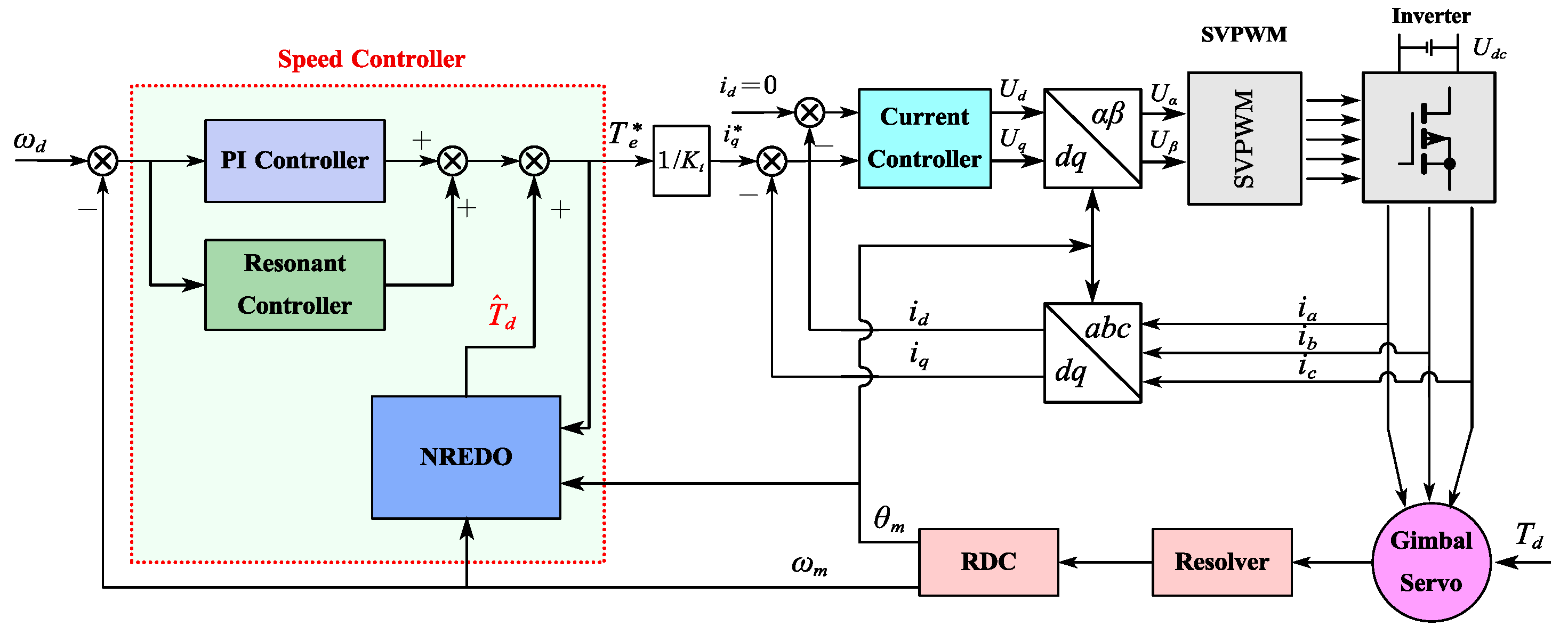
3. PIR-NREDO Controller

To suppress multiple disturbances in the gimbal servo system, the PIR-NREDO is proposed in this section. The structure of the system under the proposed method is shown in Figure 1. The speed controller consists of two parts: an NREDO and a PIR controller. The NREDO is utilized to estimate the low-frequency disturbance $T_m$, and the NREDO has a stronger noise suppression ability than an EDO of the same bandwidth. The PIR controller is composed of a PI controller and a resonant controller in parallel, where the resonant controller is adopted to suppress the high-frequency rotor dynamic imbalance torque $T_r$.

3.1. Design of NREDO

In this section, an NREDO is designed to address the sensitivity of the EDO to measurement noise. By introducing the integral of the virtual measurement of $T_d$ as an augmented state, the disturbance dynamic model is derived. This model then serves as the basis for the design of the NREDO. Afterward, the frequency domain performance is analyzed, while the selection of observer gain is discussed.

According to (1), the virtual measurement of $T_d$ is expressed as follows:

$$T_{dm}=T_e-J{\dot{\omega }}_m-D{\omega }_m$$

(9)

where $T_{dm}$ is the virtual measurement of $T_d$, and ${\omega }_m$ is the measured angular speed.

To reduce the effects of measurement noise on the observer, an integration operation is performed on $T_{dm}$, yielding the following:

$$T_{dmI}={\int }_0^t{T}_{e}d\tau -J{\omega }_m-D{\theta }_m$$

(10)

where ${\theta }_m$ is the measured angular position.

According to (1), the actual integral value of $T_d$ is expressed as follows:

$$T_{dI}={\int }_0^t{T}_{e}d\tau -J\omega -D\theta$$

(11)

The measurement error between $T_{dI}$ and $T_{dmI}$ can be derived from (10) and (11) as follows:

$$T_{dI}-T_{dmI}=-D\tilde{\theta }-J\tilde{\omega }$$

(12)

where $\tilde{\theta }=\theta -{\theta }_m$, $\tilde{\omega }=\omega -{\omega }_m$.

According to Assumption 1, by taking $T_{dmI}$ as an augmented state, and defining the state variables $x_0=T_{dmI}$, $x_1=T_d$, $x_2={\dot{T}}_d$, …, $x_n=T_d^{(n-1)}$, the $(n+1)$th-order dynamic model of $T_d$ can be expressed as follows:

$$\left\{\begin{array}{c}{\dot{x}}_0=x_1+D\tilde{\omega }+J\dot{\tilde{\omega }}\hfill \\ {\dot{x}}_i=x_{i+1},i=1,\dots ,n-1\hfill \\ {\dot{x}}_n=T_d^{\left(n\right)}\hfill \end{array}\right.$$

(13)

Taking $T_{dmI}$ as the output, the state-space equation can be derived from (13) as follows:

$$\left\{\begin{array}{c}\dot{\mathit{x}}=\mathit{A}\mathit{x}+\mathit{B}{T}_d^{\left(n\right)}+\mathit{E}(D\tilde{\omega }+J\dot{\tilde{\omega }})\hfill \\ T_{dmI}=\mathit{C}\mathit{x}\hfill \end{array}\right.$$

(14)

where $\mathit{A}=\left[\begin{array}{cc}{\mathit{O}}_{n\times 1}& {\mathit{I}}_n\\ {\mathit{O}}_{1\times 1}& {\mathit{O}}_{1\times n}\end{array}\right]$, $\mathit{B}=\left[\begin{array}{c}{\mathit{O}}_{n\times 1}\\ 1\end{array}\right]$, $\mathit{E}=\left[\begin{array}{c}1\\ {\mathit{O}}_{n\times 1}\end{array}\right]$, $\mathit{C}=\left[\begin{array}{cc}1& {\mathit{O}}_{1\times n}\end{array}\right]$, $\mathit{x}={\left[\begin{array}{cccc}{x}_0& x_1& \cdots & x_n\end{array}\right]}^{\mathrm{T}}$, and ${\mathit{O}}_{n\times n}$ denotes the $n\times n$ zero matrix.

Since $\mathrm{r}\mathrm{a}\mathrm{n}\mathrm{k}{\left[\begin{array}{cccc}\mathit{C}& \mathit{C}\mathit{A}& \cdots & \mathit{C}{\mathit{A}}^n\end{array}\right]}^{\mathrm{T}}=n+1$, (14) is observable, the $(n+1)$th-order NREDO is designed as follows:

$$\left\{\begin{array}{c}\dot{\widehat{\mathit{x}}}=\mathit{A}\widehat{\mathit{x}}+\mathit{L}(T_{dmI}-{\widehat{T}}_{dmI})\hfill \\ {\widehat{T}}_{dmI}=\mathit{C}\widehat{\mathit{x}}\hfill \end{array}\right.$$

(15)

where $\widehat{\mathit{x}}={\left[\begin{array}{cccc}{\widehat{x}}_0& {\widehat{x}}_1& \cdots & {\widehat{x}}_n\end{array}\right]}^{\mathrm{T}}$ is the estimated value of the state variable $\mathit{x}$; $\mathit{L}={\left[\begin{array}{cccc}{l}_0& l_1& \cdots & l_n\end{array}\right]}^{\mathrm{T}}$, $l_m>0$, $m=\mathrm{0,1},\dots ,n$, and $\mathit{L}$ is the observer gain matrix; and ${\widehat{T}}_{dmI}$ is the estimated value of $T_{dmI}$.

Equation (15) can be used to determine whether the observer states are updated by using the estimation error of $T_{dmI}$ instead of the estimation error of $T_{dm}$. Consequently, the NREDO can filter a significant amount of measurement noise compared with the EDO.

Substituting (10) into (15), we can obtain the following:

$$\dot{\widehat{\mathit{x}}}=(\mathit{A}-\mathit{L}\mathit{C})\widehat{\mathit{x}}+\mathit{L}({\int }_0^t{T}_{e}d\tau -D{\theta }_m-J{\omega }_m)$$

(16)

By defining the state estimation error variable $\tilde{\mathit{x}}=\mathit{x}-\widehat{\mathit{x}}$, the error dynamic equation of the NREDO can be derived from (14) and (15) as follows:

$$\dot{\tilde{\mathit{x}}}=(\mathit{A}-\mathit{L}\mathit{C})\tilde{\mathit{x}}+\mathit{B}{T}_d^{\left(n\right)}+\mathit{E}(D\tilde{\omega }+J\dot{\tilde{\omega }})$$

(17)

Then, the frequency domain performance of the NREDO can be analyzed. Since $x_1=T_d$, the Laplace transform of (17) under zero initial conditions can be expressed as follows:

$${\tilde{T}}_d(s)={\displaystyle \frac{s^n(s+l_0)}{\lambda \left(s\right)}}{T}_d(s)-{\displaystyle \frac{(l_1{s}^{n-1}+\cdots +l_n)(Js+D)}{\lambda \left(s\right)}}\tilde{\omega }(s)$$

(18)

where $\lambda \left(s\right)=s^{n+1}+l_0{s}^n+l_1{s}^{n-1}+\cdots +l_n$.

Equation (18) can be expressed as follows:

$${\tilde{T}}_d(s)=G_{{\tilde{T}}_d/T_d}(s)T_d(s)+G_{{\tilde{T}}_d/n_{\omega }}(s)n_{\omega }(s)$$

(19)

where $n_{\omega }(s)=(Js+D)\tilde{\omega }(s)$ is the measurement noise, $G_{{\tilde{T}}_d/T_d}\left(s\right)$ represents the effects of $T_d(s)$ on the disturbance estimation accuracy, and $G_{{\tilde{T}}_d/n_{\omega }}\left(s\right)$ represents the effects of the measurement noise $n_{\omega }(s)$ on the disturbance estimation accuracy.

The transfer functions $G_{{\tilde{T}}_d/T_d}(s)$ and $G_{{\tilde{T}}_d/n_{\omega }}(s)$ are expressed as follows:

$$G_{{\tilde{T}}_d/T_d}\left(s\right)={\displaystyle \frac{s^n(s+l_0)}{\lambda \left(s\right)}}$$

(20)

$$G_{{\tilde{T}}_d/n_{\omega }}\left(s\right)={\displaystyle \frac{(l_1{s}^{n-1}+\cdots +l_n)}{\lambda \left(s\right)}}$$

(21)

To facilitate frequency domain performance analysis, ${\omega }_o$ is defined as the bandwidth of the NREDO. By configuring the poles of (20) and (21) as $(n+1)$-times multiple roots of ${-\omega }_o$, the system characteristic polynomial $\lambda \left(s\right)$ can be rewritten as follows:

$$\lambda \left(s\right)=(s+{\omega }_o{)}^{n+1}$$

(22)

The observer gain can be obtained using the method of undetermined coefficients, as follows:

$$l_m=C_{n+1}^{m+1}{\omega }_o^{m+1},m=\mathrm{0,1},\dots ,n$$

(23)

where $C_n^m=n!/(m!(n-m)!)$.

Then, $G_{{\tilde{T}}_d/T_d}(s)$ and $G_{{\tilde{T}}_d/n_{\omega }}\left(s\right)$ can be expressed as follows:

$$G_{{\tilde{T}}_d/T_d}\left(s\right)={\displaystyle \frac{s^n\left[s+(n+1){\omega }_o\right]}{(s+{\omega }_o{)}^{n+1}}}$$

(24)

$$G_{{\tilde{T}}_d/n_{\omega }}\left(s\right)={\displaystyle \frac{\sum _{m=1}^n{C}_{n+1}^{m+1}{\omega }_o^{m+1}{s}^{n-m}}{(s+{\omega }_o{)}^{n+1}}}$$

(25)

According to (24) and (25), amplitude–frequency characteristic curves can be plotted. To evaluate the performance of the NREDO, the EDO and NREDO use the same bandwidth and parameter conditions. The amplitude–frequency characteristic curves of $G_{{\tilde{T}}_d/T_d}\left(s\right)$ and $G_{{\tilde{T}}_d/n_{\omega }}\left(s\right)$ are shown in Figure 2a,b, respectively.

As shown in Figure 2a, the disturbance estimation ability of the NREDO is decreased compared with the EDO of the same order. As the order increases, the disturbance estimation abilities of both improve. As shown in Figure 2b, the NREDO exhibits lower sensitivity to measurement noise and demonstrates enhanced robustness against noises compared with the EDO of the same order. As the order increases, both observers show a slightly decrease in noise attenuation capability. Although the NREDO sacrifices some disturbance rejection performance, it achieves a marked improvement in noise reduction. In practical applications, the bandwidth ${\omega }_o$ needs to be tuned. Then, the gain matrix is obtained according to (23). Since the frequency of $T_m$ is relatively low, a large value of ${\omega }_o$ is not required.

3.2. Design of PIR Controller

The NREDO cannot accurately estimate the rotor dynamic imbalance torque $T_r$, because $T_r$ has a much higher frequency compared with other disturbances, according to (7). Actually, the bandwidth of the NREDO is much smaller than $T_r$. Therefore, a resonant controller with phase compensation is utilized to suppress $T_r$. The PIR controller consists of a resonant controller in parallel with a PI controller. The transfer function of the PIR controller is designed as follows:

$$G_{PIR}(s)=G_{PI}(s)+G_R(s)$$

(26)

where the PI controller $G_{PI}(s)=K_p+K_i/s$ and the resonant controller $G_R(s)$ can be expressed as follows [19]:

$$G_R(s)=K_r{\displaystyle \frac{s\cos {\varphi }_r-{\omega }_r\sin {\varphi }_r}{s^2+{\omega }_r^2}}$$

(27)

where $K_r$ is the resonant gain, ${\varphi }_r$ is the compensation phase, and ${\omega }_r$ is the resonant frequency.

According to (27), the resonant controller has a sufficiently large gain at the resonant frequency. Therefore, the resonant controller can be utilized to suppress the high-frequency periodic disturbance. In addition, the system’s stability margin at the resonant frequency can be improved by introducing the compensation phase ${\varphi }_r$.

The parameters of the PIR controller can be tuned as follows: First, the PI part is tuned. Letting $K_r=0$, $K_p$ is tuned to improve dynamic response of the gimbal servo system. Then, $K_i$ is gradually increased to eliminate steady-state error. Second, the resonant part is tuned. Keeping the PI part unchanged, and letting ${\omega }_r$ be the frequency to be suppressed, the compensation phase ${\varphi }_r$ has a relatively high value. Based on this, the resonant gain $K_r$ is gradually increased until the rotor imbalance disturbance is effectively suppressed. The tuned parameters are shown in

Table 1. The parameters of the PIR controller.

Parameters	${\mathit{K}}_{\mathit{p}}$	${\mathit{K}}_{\mathit{i}}$	${\mathit{K}}_{\mathit{r}}$	${\mathit{\varphi }}_{\mathit{r}}\left(°/\mathbf{s}\right)$	${\mathit{\omega }}_{\mathit{r}}(\mathbf{r}\mathbf{a}\mathbf{d}/\mathbf{s})$
Values	5	50	430	220	$200\mathsf{\pi }$

.

According to the tuned parameters in Table 1, the bode diagram of the closed-loop system in Figure 1 is shown in Figure 3. It can be observed that PIR controller retains the performance of the PI controller, while improving the suppression of the periodic disturbance at the resonant frequency.

3.3. Stability Proof

According to (17), the error dynamic equation of the NREDO can be expressed as follows:

$$\dot{\tilde{\mathit{x}}}={\mathit{A}}_o\tilde{\mathit{x}}+\mathit{B}{T}_d^{\left(n\right)}+\mathit{E}{n}_{\omega }$$

(28)

where ${\mathit{A}}_o=\mathit{A}-\mathit{L}\mathit{C}$.

The error variable is defined as ${\tilde{\omega }}_m={\omega }_d-{\omega }_m$, ${\tilde{\theta }}_m={\theta }_d-{\theta }_m$, where ${\omega }_d$ is the desired gimbal angular speed, and ${\theta }_d$ is the desired gimbal angular position. According to (9), the system state equation can be expressed as follows:

$$\left\{\begin{array}{c}{\dot{\tilde{\theta }}}_m={\tilde{\omega }}_m\hfill \\ {\dot{\tilde{\omega }}}_m=-{\displaystyle \frac{T_e^{*}}{J}}-{\displaystyle \frac{D}{J}}{\tilde{\omega }}_m+{\displaystyle \frac{T_{dm}}{J}}+{\displaystyle \frac{D}{J}}{\omega }_d+{\dot{\omega }}_d\hfill \end{array}\right.$$

(29)

where $T_e^{*}$ is the desired electromagnetic torque.

$T_e^{*}$ is designed as follows:

$$T_e^{*}=u_{PI}+u_R+{\widehat{T}}_d$$

(30)

where $u_{PI}$ is the output of the PI controller, and $u_R$ is the output of the resonant controller.

$u_{PI}$ can be expressed as follows:

$$u_{PI}=K_p{\tilde{\omega }}_m+K_i{\tilde{\theta }}_m$$

(31)

According to (27), the state-space equation of the resonant controller can be expressed as follows:

$$\left\{\begin{array}{c}\left[\begin{array}{c}{\dot{x}}_{r1}\\ {\dot{x}}_{r2}\end{array}\right]=\left[\begin{array}{cc}0& 1\\ -{\omega }_r^2& 0\end{array}\right]\left[\begin{array}{c}{x}_{r1}\\ x_{r2}\end{array}\right]+\left[\begin{array}{c}0\\ 1\end{array}\right]{\tilde{\omega }}_m\\ u_R=\left[\begin{array}{cc}-K_r{\omega }_r{\sin \varphi }_r& K_r{\cos \varphi }_r\end{array}\right]\left[\begin{array}{c}{x}_{r1}\\ x_{r2}\end{array}\right]\end{array}\right.$$

(32)

where $x_{r1}$ and $x_{r2}$ are the states of the resonant controller.

Substituting (30) and (31) into the second equation of (29), we can obtain the following:

$$\begin{array}{ll}{\dot{\tilde{\omega }}}_m& =-{\displaystyle \frac{1}{J}}\left(u_{PI}+u_R+{\widehat{T}}_d\right)-{\displaystyle \frac{D}{J}}{\tilde{\omega }}_m+{\displaystyle \frac{T_{dm}}{J}}+{\displaystyle \frac{D}{J}}{\omega }_d+{\dot{\omega }}_d\\ & =-{\displaystyle \frac{K_i}{J}}{\tilde{\theta }}_m-{\displaystyle \frac{K_p+D}{J}}{\tilde{\omega }}_m-{\displaystyle \frac{u_R}{J}}+{\displaystyle \frac{{\tilde{T}}_d}{J}}+{\displaystyle \frac{D}{J}}{\omega }_d+{\dot{\omega }}_d+{\displaystyle \frac{n_{\omega }}{J}}\end{array}$$

(33)

In addition, ${\tilde{x}}_1={\tilde{T}}_d$. Substituting (32) into (33) and simplifying, ${\dot{\tilde{\omega }}}_m$ is expressed as follows:

$${\dot{\tilde{\omega }}}_m=-{\displaystyle \frac{K_i}{J}}{\tilde{\theta }}_m-{\displaystyle \frac{K_p+D}{J}}{\tilde{\omega }}_m+{\displaystyle \frac{K_r{\omega }_r{\sin \varphi }_r}{J}}{x}_{r1}-{\displaystyle \frac{K_r{\cos \varphi }_r}{J}}{x}_{r2}+{\displaystyle \frac{{\tilde{x}}_1}{J}}+{\displaystyle \frac{D}{J}}{\omega }_d+{\dot{\omega }}_d+{\displaystyle \frac{n_{\omega }}{J}}$$

(34)

According to (28), (29), and (34), the closed-loop system can be expressed as follows:

$$\left[\begin{array}{c}{\dot{\tilde{\theta }}}_m\\ {\dot{\tilde{\omega }}}_m\\ \begin{array}{c}{\dot{x}}_{r1}\\ \begin{array}{c}{\dot{x}}_{r2}\\ \stackrel{¯\; ¯\; ¯\; ¯\; ¯}{\dot{\tilde{\mathit{x}}}}\end{array}\end{array}\end{array}\right]=\left[\begin{array}{cc}{\mathit{A}}_s& {\mathit{A}}_J\\ {\mathit{O}}_{(n+1)\times 4}& {\mathit{A}}_o\end{array}\right]\left[\begin{array}{c}{\tilde{\theta }}_m\\ {\tilde{\omega }}_m\\ \begin{array}{c}{x}_{r1}\\ \begin{array}{c}{x}_{r2}\\ \stackrel{¯\; ¯\; ¯\; ¯\; ¯}{\tilde{\mathit{x}}}\end{array}\end{array}\end{array}\right]+\left[\begin{array}{ccc}0& 0& 0\\ 1& {\displaystyle \frac{1}{J}}& 0\\ 0& 0& 0\\ 0& 0& 0\\ {\mathit{O}}_{(n+1)\times 1}& \mathit{E}& \mathit{B}\end{array}\right]\left[\begin{array}{c}{\displaystyle \frac{D{\omega }_d}{J}}+{\dot{\omega }}_d\\ n_{\omega }\\ T_d^{\left(n\right)}\end{array}\right]$$

(35)

where ${\mathit{A}}_s=\left[\begin{array}{cccc}0& 1& 0& 0\\ -{\displaystyle \frac{K_i}{J}}& -{\displaystyle \frac{K_p+D}{J}}& {\displaystyle \frac{K_r{\omega }_r{\sin \varphi }_r}{J}}& -{\displaystyle \frac{K_r{\cos \varphi }_r}{J}}\\ 0& 0& 0& 1\\ 0& 1& -{\omega }_r^2& 0\end{array}\right]$, ${\mathit{A}}_J=\left[\begin{array}{ccccc}0& 0& 0& \cdots & 0\\ 0& {\displaystyle \frac{1}{J}}& 0& \cdots & 0\\ 0& 0& 0& \cdots & 0\\ 0& 0& 0& \cdots & 0\end{array}\right]$.

The eigenvalues of the system can be derived according to (36). It can be observed that the eigenvalues depend on ${\mathit{A}}_s$ and ${\mathit{A}}_o$. Notably, the eigenvalues of ${\mathit{A}}_o$ are all equal to ${-\omega }_o$, according to (22). Similarly, the eigenvalues of ${\mathit{A}}_s$ can also be placed in the left plane. Therefore, system stability can be ensured.

$$\lambda \left(\left[\begin{array}{cc}{\mathit{A}}_s& {\mathit{A}}_J\\ {\mathit{O}}_{(n+1)\times 4}& {\mathit{A}}_o\end{array}\right]\right)=\lambda \left({\mathit{A}}_s\right)\cup \lambda \left({\mathit{A}}_o\right)$$

(36)

where $\lambda \left(·\right)$ denotes eigenvalues of the matrix $\left(·\right)$.

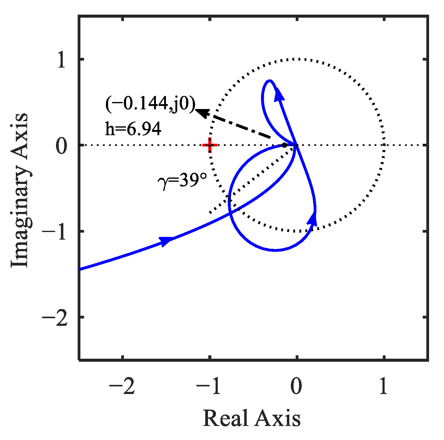
3.4. Stability Margin

To evaluate the system stability margins, the block diagram of the control system in Figure 1 can be simplified as shown in Figure 4. The current loop has a relatively high bandwidth compared with the speed loop, and its transfer function can be approximated as 1.

In Figure 4, the controlled object $G_P(s)=1/(Js+D)$. The speed measurement value ${\omega }_m$ is obtained from the RDC output value ${\theta }_m$ through backward differentiation. For convenience, the transfer function $G_m(s)$ is expressed as follows:

$$G_m(s)={\displaystyle \frac{1}{1+b{T}_{s}s}}$$

(37)

where $T_s$ is the sampling period, and $b$ is the ratio of the differential time interval to the sampling period.

In this paper, AD2S1210 (Analog Devices, Wilmington, MA, USA) is utilized as the RDC, and its transfer function is expressed as follows [31]:

$$G_{RDC}(s)={\displaystyle \frac{k_a{t}_{1}s+k_a}{t_2{s}^3+s^2+k_a{t}_{1}s+k_a}}$$

(38)

where $k_a$, $t_1$, and $t_2$ are constant parameters set according to the user manual.

The control system is equivalent to a unit negative feedback system. The open-loop transfer function $G_o(s)$ of the system is expressed as follows:

$$G_o(s)=G_{PIR}(s)G_P(s)G_{RDC}(s)G_m(s)$$

(39)

Then, the characteristic polynomial of (39) is derived as follows:

$${\lambda }_o(s)=s(s^2+{\omega }_r^2)(Js+D)(t_2{s}^3+s^2+k_a{t}_{1}s+k_a)(1+b{T}_{s}s)$$

(40)

The parameters of the RDC are set according to the user manual, as follows: $k_a=92.7\times {10}^3$, $t_1=8\times {10}^{-3}$, $t_2=728\times {10}^{-6}$. Plant parameters are set according to the experimental system, as follows: $J=0.6821\mathrm{k}\mathrm{g}·{\mathrm{m}}^2$, $D=0.008\mathrm{N}\mathrm{m}/(\mathrm{r}\mathrm{a}\mathrm{d}·{\mathrm{s}}^{-1})$. The parameters of the PIR controller are shown in Table 1. Below, a Nyquist diagram of the open-loop transfer function $G_o(s)$ is shown in Figure 5.

As shown in Figure 5, the gain margin is 6.94 and the phase margin is 39°. While ensuring system stability, the controller parameters should be tuned to move the Nyquist diagram away from the point $(-1,\mathrm{j}0)$ to improve stability margins.

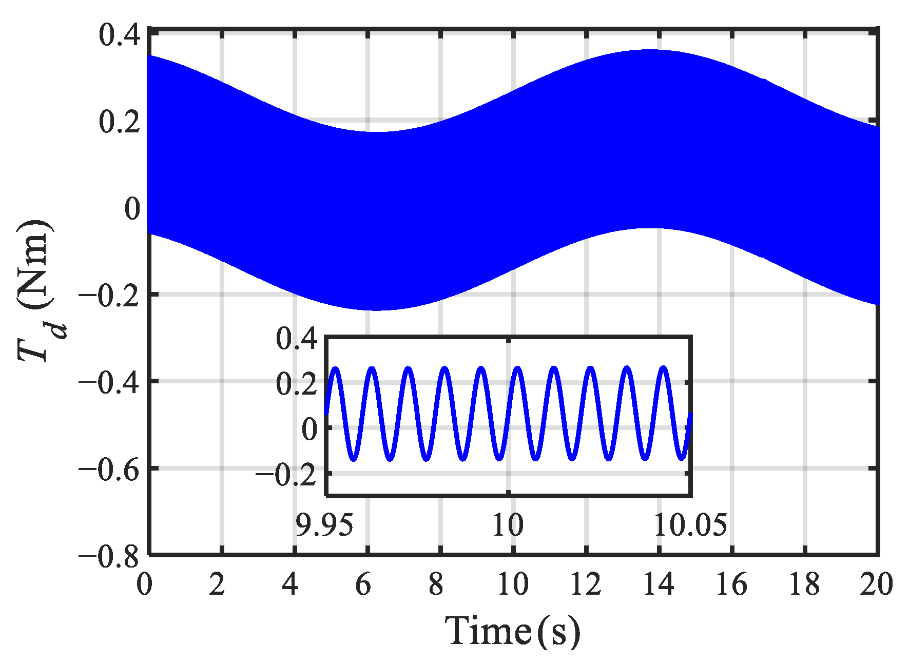
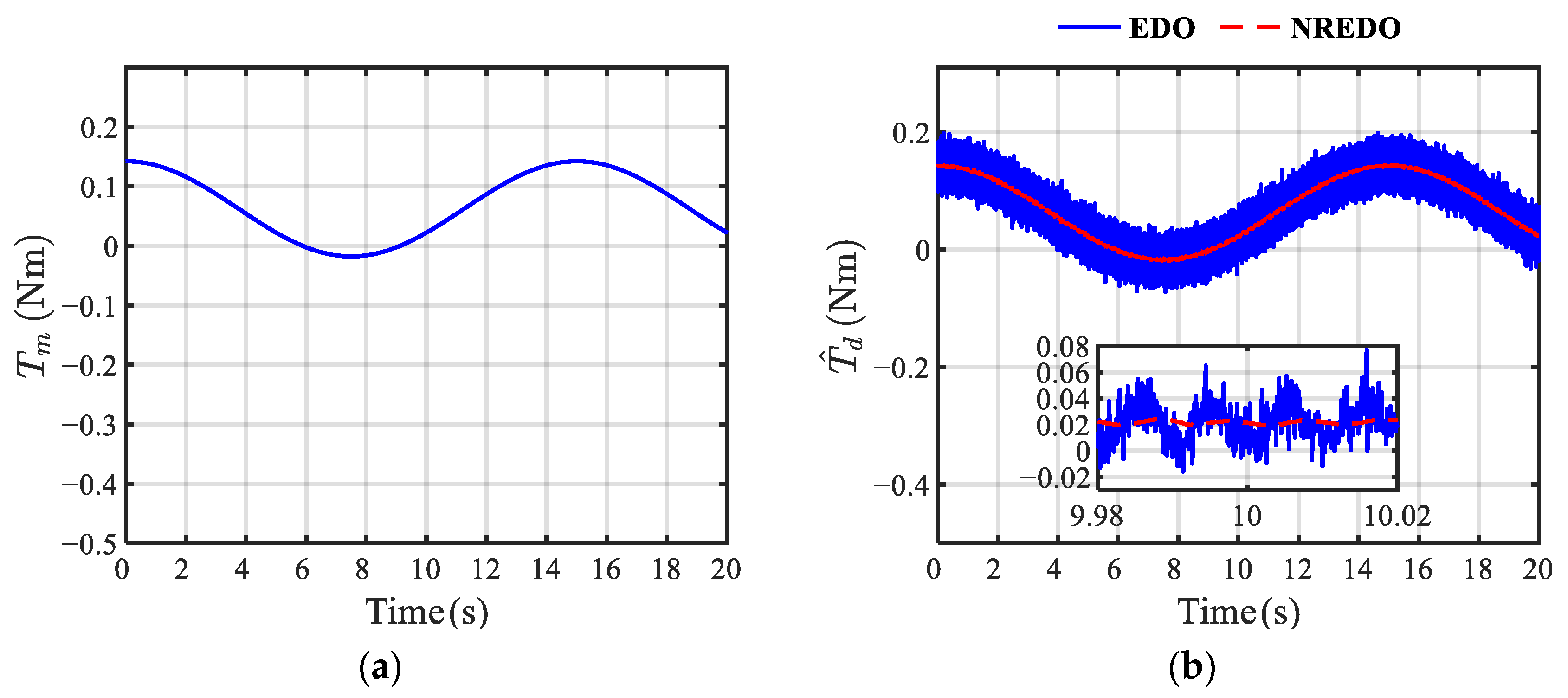
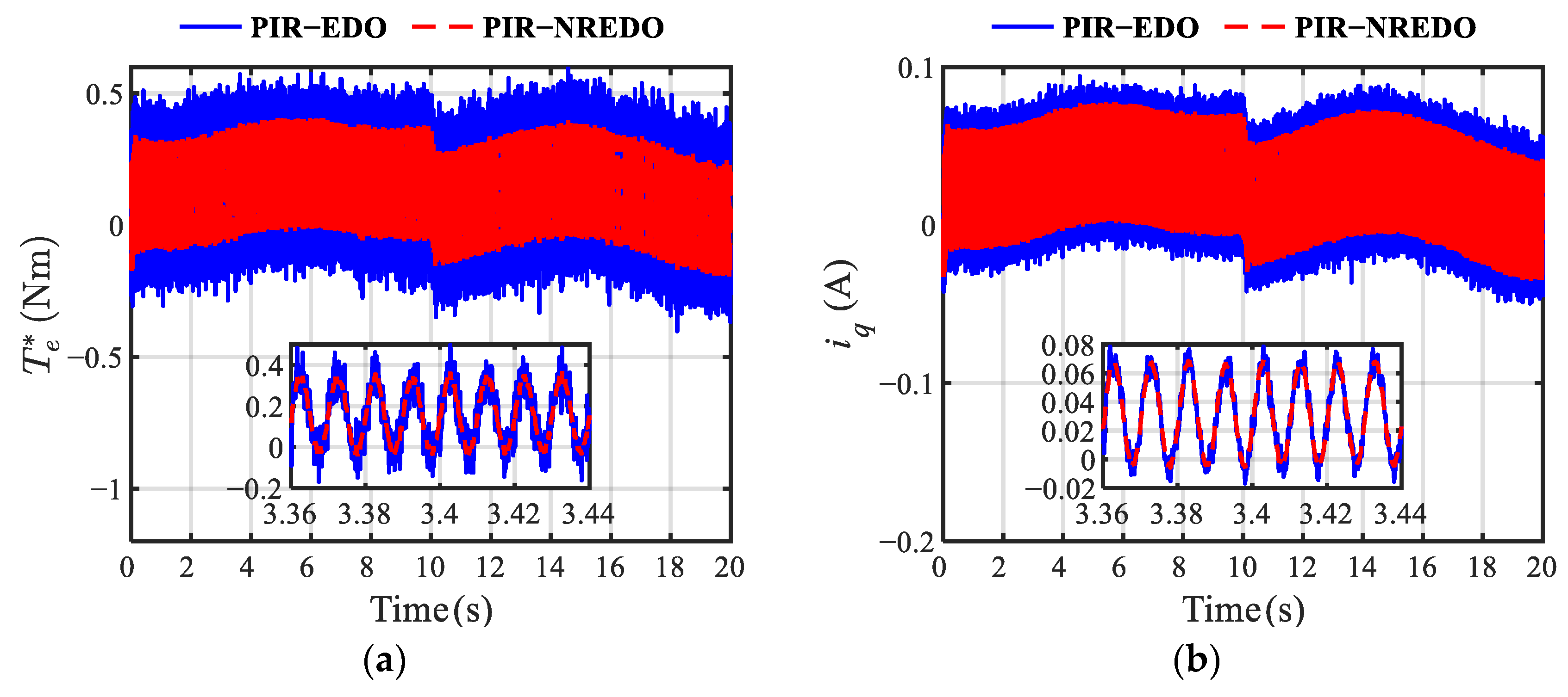
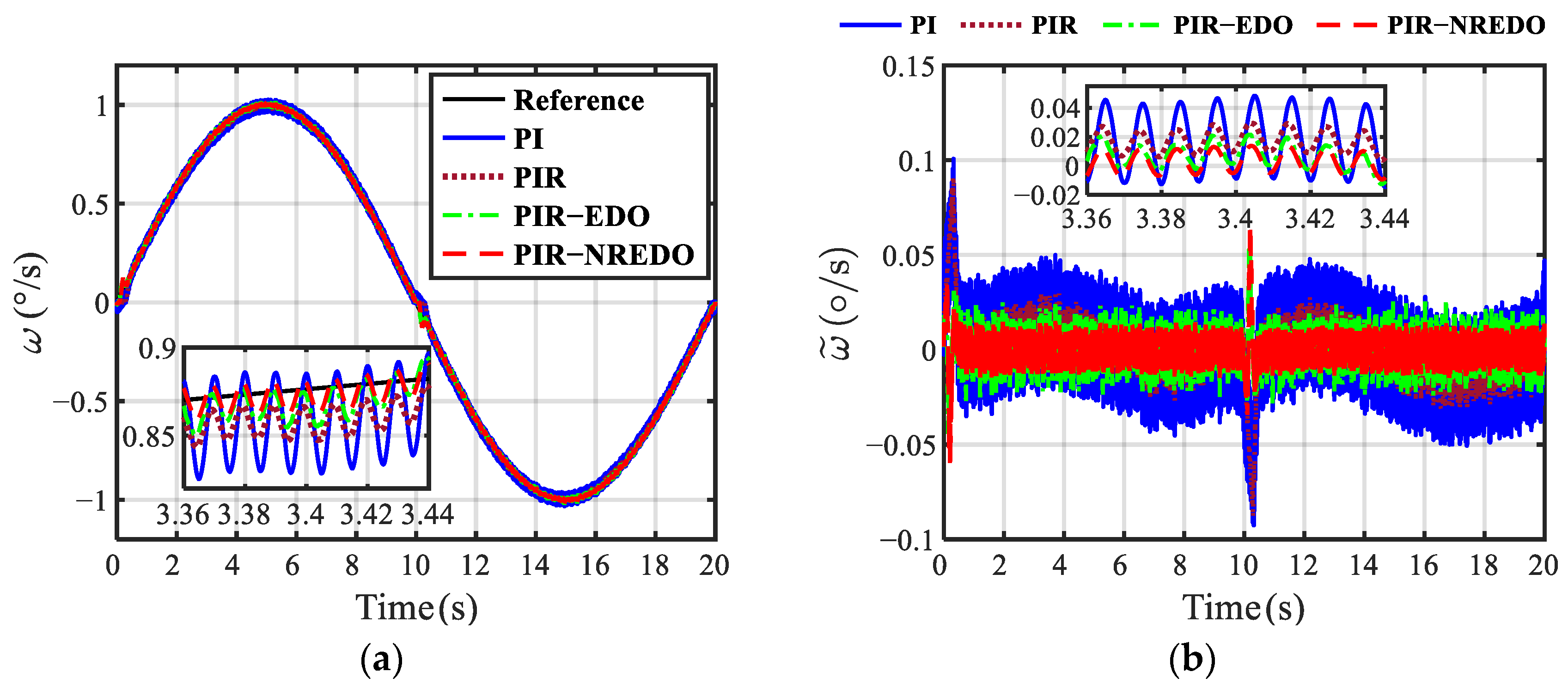
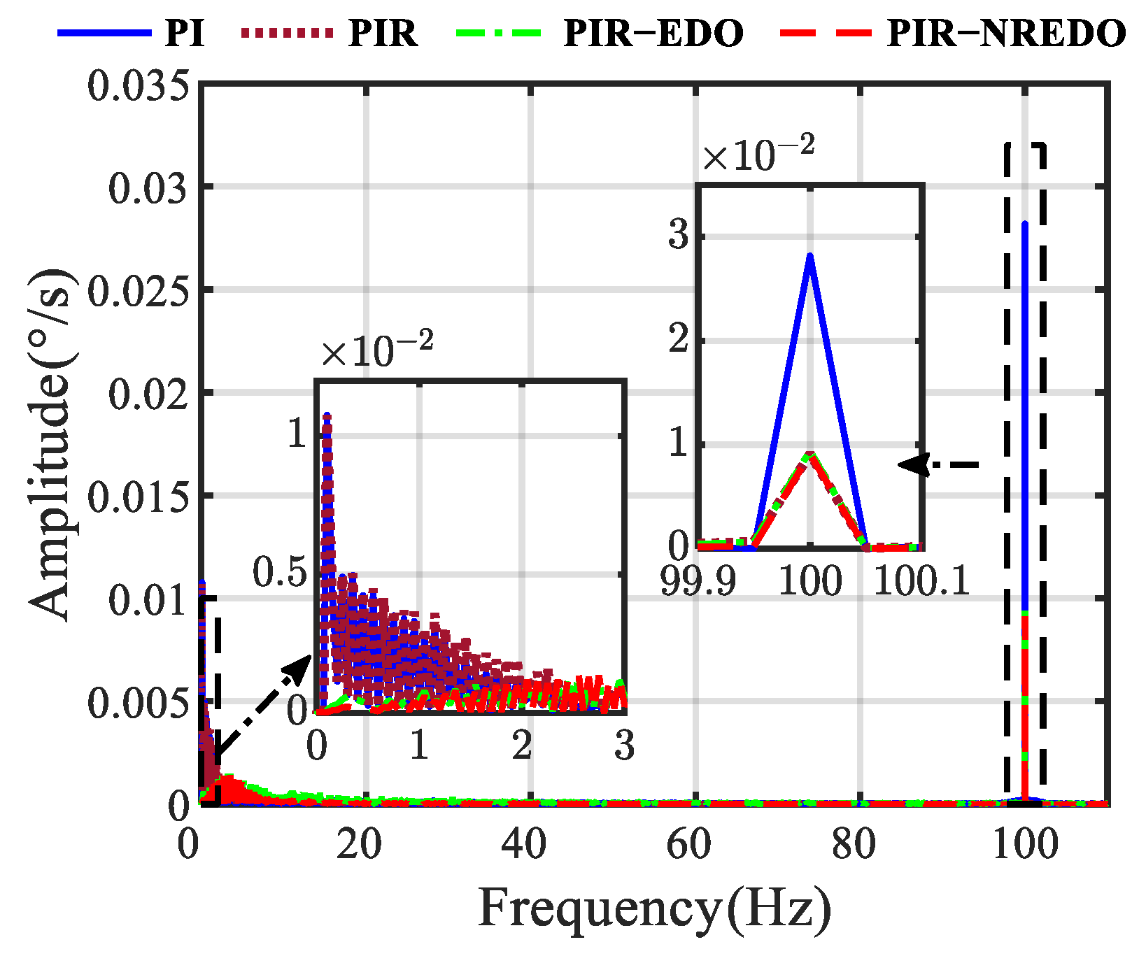
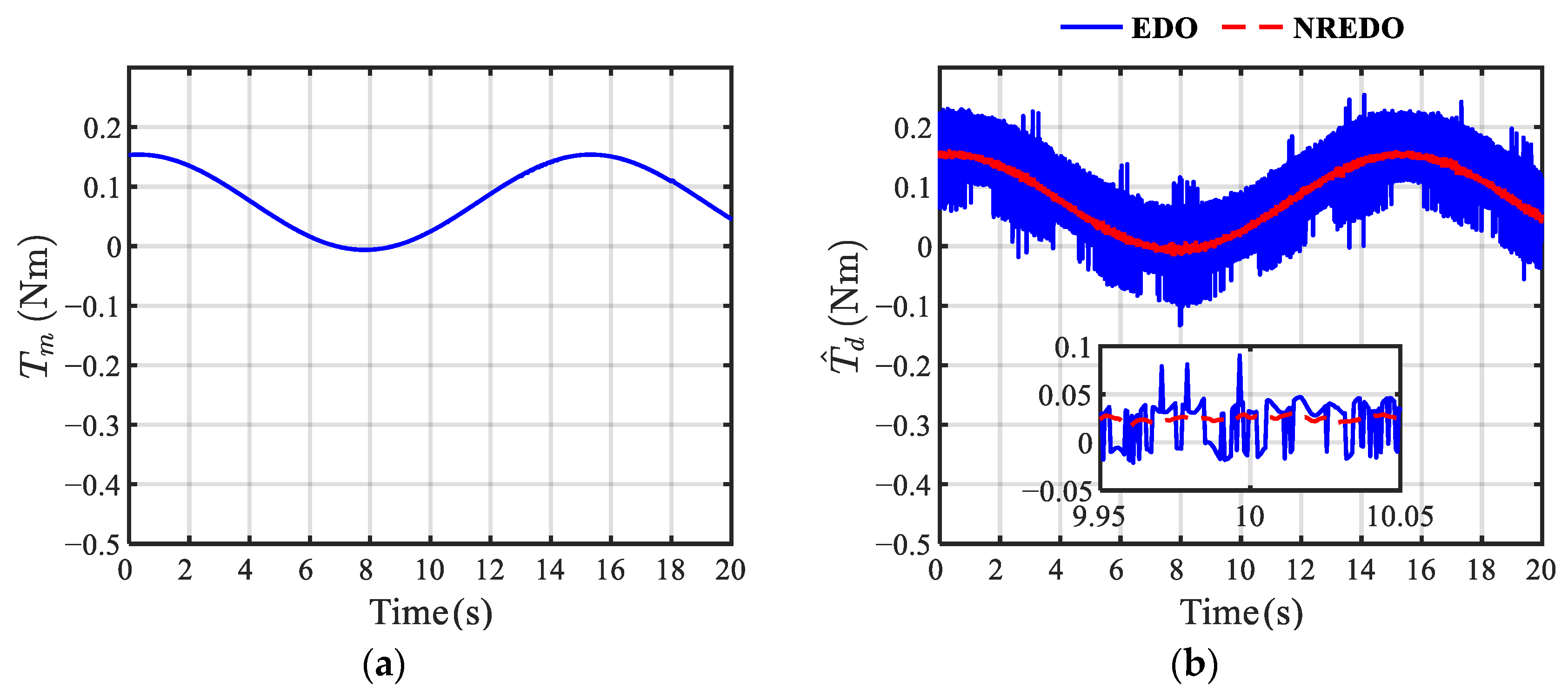
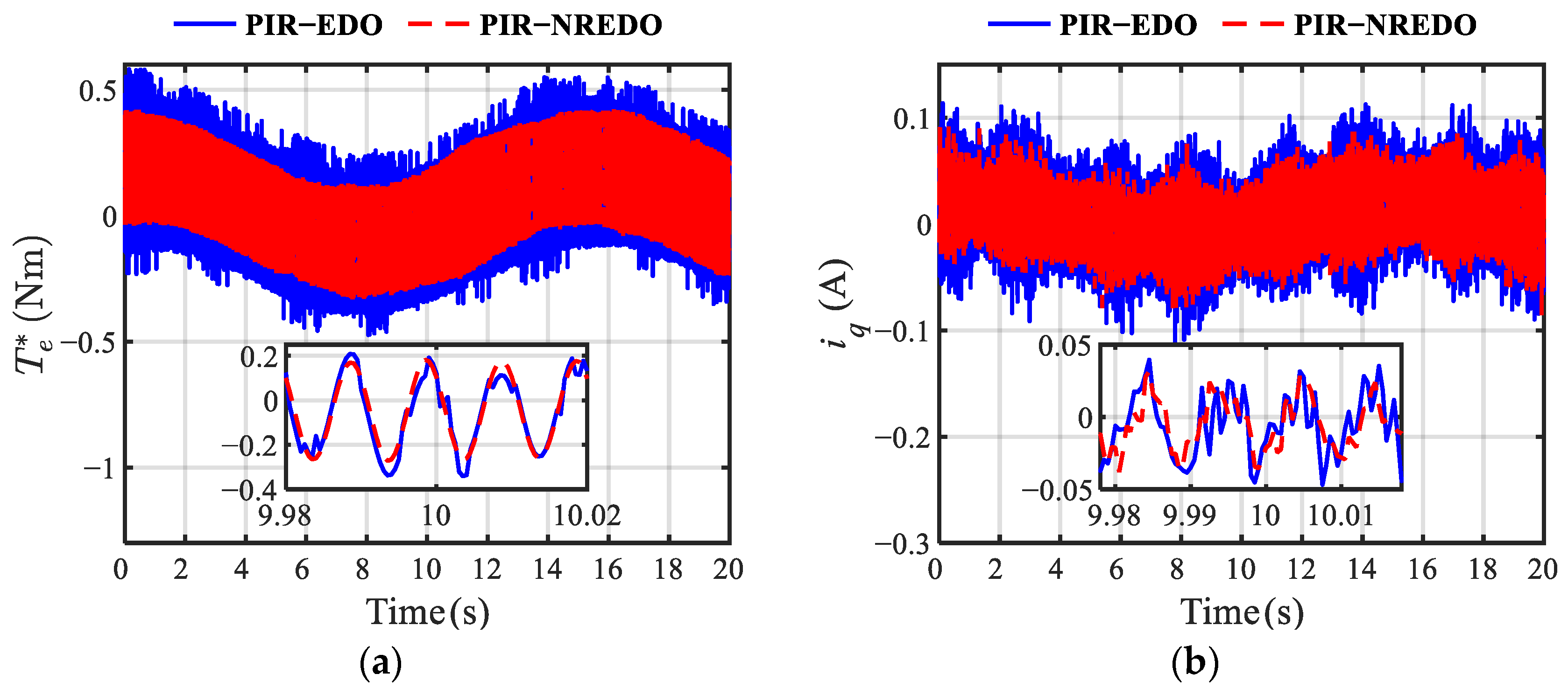
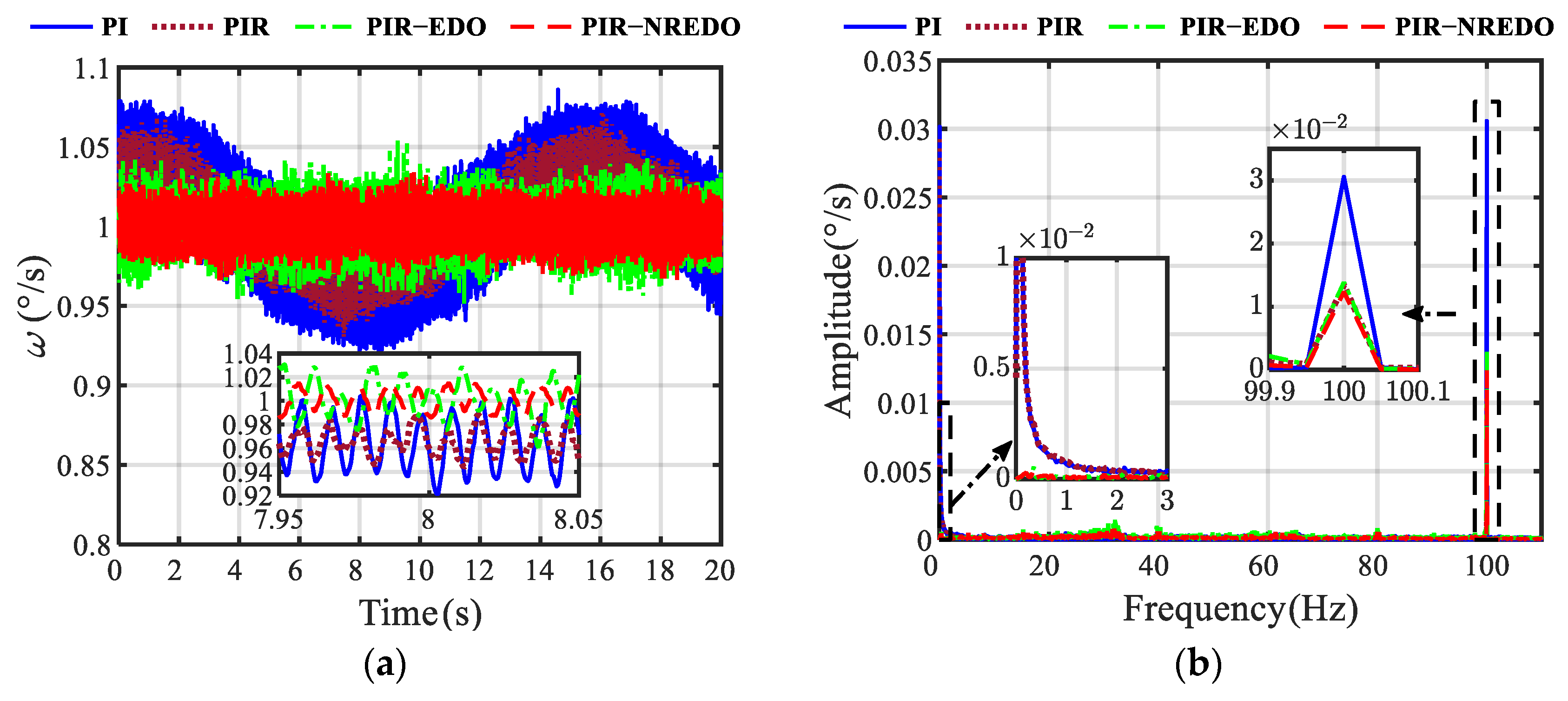
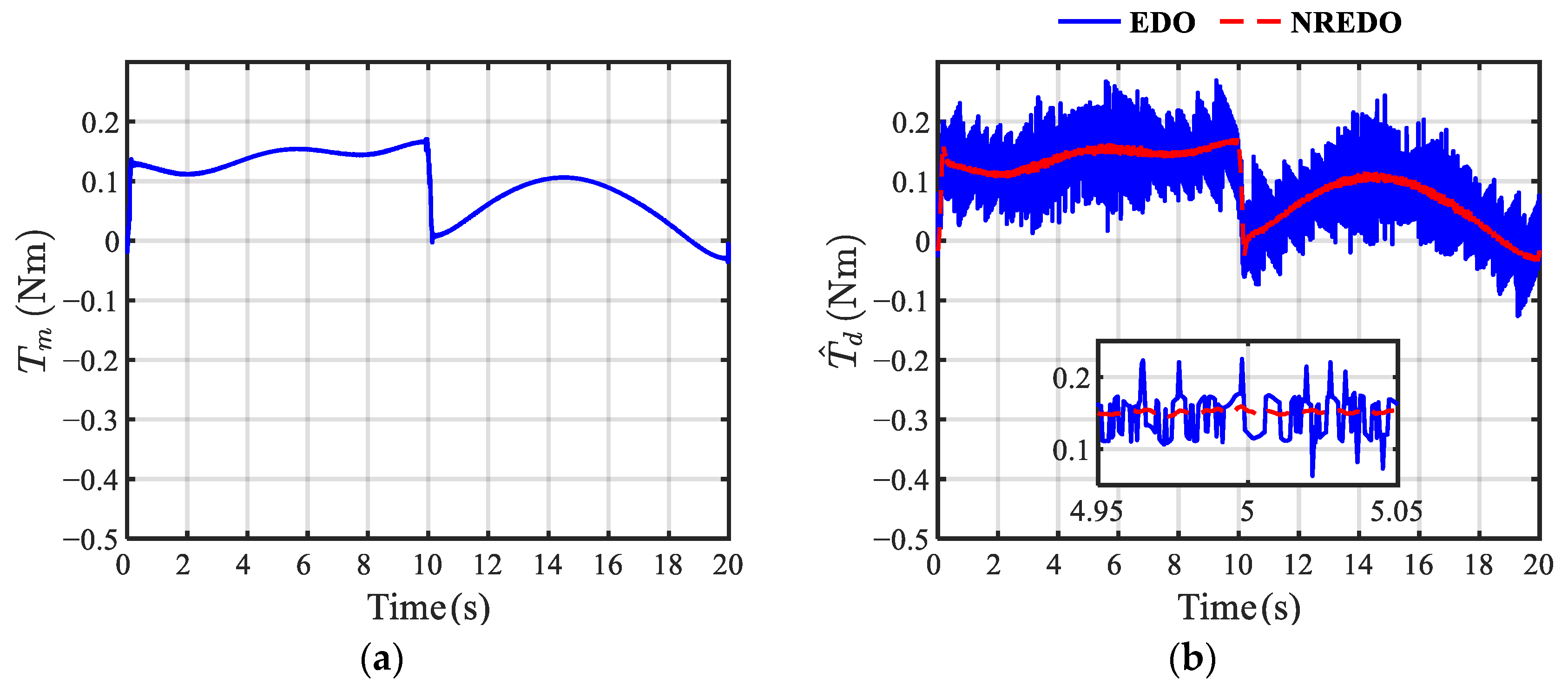
4. Simulation Results

To validate the effectiveness of the proposed method, numerical simulation was conducted using four different control methods, i.e., PI, PIR, PIR-EDO, and PIR-NREDO. The gimbal servo system was set to track two different desired speeds: a fixed speed and a sinusoidal speed. A simulation model was built in MATLAB(R2023b)/Simulink according to Figure 1. The parameters of the gimbal servo system used in the model are shown in

Table 2. The parameters of the gimbal servo system.

Parameters	Values
Moment of inertia	0.6821 kg⋅m2
Damping coefficient	0.008 Nm/(rad⋅s−1)
Torque coefficient	5 Nm/A
Back EMF coefficient	5 V(rad/s)
Pole pairs	6
Phase inductance	14.5 mH
Phase resistance	2.5 Ω

. The disturbance parameters were set as shown in

Table 3. Disturbance parameters in simulation.

Parameters	Values	Parameters	Values
$F_c$(Nm)	0.01	$T_1$(Nm)	0.08
$F_s$ (Nm)	0.04	$N_{cog}$	24
$F_v$ (Nm)	0.05	$u_d$(g⋅cm2)	5.066
${\omega }_s$(rad/s)	0.01	$\Omega$(rpm)	6000

. Additionally, Gaussian white noise with an average amplitude of $5\times 10^{-4}°/\mathrm{s}$ was added to the gimbal angular speed. The current controllers of the d-axis and q-axis were both PI controllers. The transfer function of current controllers can be expressed as follows:

$$U_d\left(s\right)=K_{pd}+{\displaystyle \frac{K_{id}}{s}}$$

(41)

$$U_q\left(s\right)=K_{pq}+{\displaystyle \frac{K_{iq}}{s}}$$

(42)

where $K_{pd}$ and $K_{pq}$ are the proportional coefficients of the d-axis and q-axis current controllers, respectively; and $K_{id}$ and $K_{iq}$ are the integral coefficients of the d-axis and q-axis current controllers, respectively.

To facilitate the comparison of the EDO and NREDO, the $(n+1)$th-order EDO can be expressed as follows:

$$\left\{\begin{array}{l}\dot{\widehat{\mathit{z}}}={\mathit{A}}_{\mathit{E}}\widehat{\mathit{z}}+{\mathit{L}}_{\mathit{E}}(T_{dm}-{\widehat{T}}_{dm})\\ {\widehat{T}}_{dm}={\mathit{C}}_{\mathit{E}}\widehat{\mathit{z}}\end{array}\right.$$

(43)

where the observer states are $\widehat{\mathit{z}}={\left[\begin{array}{cccc}{\widehat{T}}_d& {\widehat{\dot{T}}}_d& \cdots & {\widehat{T}}_d^{(n+1)}\end{array}\right]}^{\mathrm{T}}$, ${\mathit{A}}_{\mathit{E}}=\left[\begin{array}{cc}{\mathit{O}}_{n\times 1}& {\mathit{I}}_n\\ {\mathit{O}}_{1\times 1}& {\mathit{O}}_{1\times n}\end{array}\right]$, and ${\mathit{C}}_{\mathit{E}}=\left[\begin{array}{cc}1& {\mathit{O}}_{1\times n}\end{array}\right]$; the observer gain matrix is ${\mathit{L}}_{\mathit{E}}={\left[\begin{array}{cccc}{l}_{E,1}& l_{E,2}& \cdots & l_{E,n+1}\end{array}\right]}^{\mathrm{T}}$; and ${\widehat{T}}_{dm}$ is the estimated value of $T_{dm}$.

It can be observed from (43) that the observer states of the EDO are updated by utilizing the estimation error of $T_{dm}$. Consequently, the measurement noise will be significantly amplified by the observer gain matrix ${\mathit{L}}_{\mathit{E}}$ compared with the NREDO.

The parameters of the PIR controller are shown in Table 1. The bandwidth of the NREDO is set as ${\omega }_o=10\mathsf{\pi }\mathrm{r}\mathrm{a}\mathrm{d}/\mathrm{s}$. Notably, the bandwidth ${\omega }_o$ and the gain matrices of the third-order EDO and the third-order NREDO are set to be the same. The parameters of the current loop PI controllers of the d-axis and q-axis are set as $K_{pd}=K_{pq}=20$ and $K_{id}=K_{iq}=0.2$.

Case 1: Fixed Speed: The gimbal angular speed is set as ${\omega }_d=1°/\mathrm{s}$; the numerical simulation curves at fixed speed are presented in Figure 6, Figure 7, Figure 8 and Figure 9. The lumped disturbance $T_d$ is shown in Figure 6. $T_d$ consists of the 100 Hz high-frequency disturbance $T_r$ and the low-frequency disturbance $T_m$. As shown in Figure 6, $T_r$ has a large amplitude.

The low-frequency disturbance $T_m$ is shown in Figure 7a. $T_m$ is estimated utilizing the EDO and NREDO, respectively, as shown in Figure 7b. The disturbance estimation result of the EDO is severely affected by measurement noise, whereas the NREDO obviously improves the signal-to-noise ratio. This indicates that the NREDO has an improved noise attenuation ability compared to the EDO of the same bandwidth. The simulation results are consistent with the frequency-domain performance analysis in Section 3.1.

The electromagnetic torque and q-axis current under the PIR-EDO and PIR-NREDO are shown in Figure 8. During the control process, the disturbance estimation result ${\widehat{T}}_d$ is directly fed forward to the desired electromagnetic torque $T_e^{*}$. Consequently, the PIR-EDO has a higher distortion in the electromagnetic torque, as shown in Figure 8a, because the estimation noise of the EDO is much higher than that of the NREDO. In addition, due to the high bandwidth of the current loop, the noise in ${\widehat{T}}_d$ will also be amplified, causing a high-frequency current ripple, as shown in Figure 8b.

The speed control results of the gimbal angular speed are shown in Figure 9. As shown in Figure 9a, the gimbal angular speed for the PIR controller has a smaller high-frequency fluctuation compared with the PI controller. This indicates that the resonant controller can effectively suppress $T_r$. However, the PIR controller has limited rejection ability for $T_m$. Consequently, the speed still includes low-frequency fluctuation. Subsequently, the EDO is added to the PIR controller to enhance the estimation of $T_m$. Then, the low-frequency speed fluctuation is obviously suppressed. Furthermore, the NREDO can mitigate the influence of measurement noises compared with the EDO. It can be observed from Figure 9a that the PIR-NREDO has the smallest angular speed fluctuation under multiple disturbances. As shown in Figure 9b, the FFT results demonstrate that the resonant controller can significantly suppress the 100 Hz high-frequency periodic disturbance. Moreover, the suppression of low-frequency disturbances is improved with the inclusion of both the EDO and NREDO. Notably, the NREDO has better noise attenuation performance compared with the EDO, as can also be observed in Figure 9a.

Case 2: Sinusoidal Speed: The gimbal angular speed is set as ${\omega }_d=\mathrm{s}\mathrm{i}\mathrm{n}\left(\mathsf{\pi }t/10\right)°/\mathrm{s}$. Numerical simulation curves at sinusoidal speed are presented in Figure 10, Figure 11, Figure 12, Figure 13 and Figure 14. Figure 10 shows the lumped disturbance at sinusoidal speed. Due to the nonlinearity of the friction torque $T_f$, there is a sudden change when the speed crosses zero. Figure 11 shows that measurement noise is obviously reduced by the NREDO. In addition, the PIR-NREDO significantly decreases the high-frequency ripple caused by the measurement noise in $T_e^{*}$ and $i_q$, as shown in Figure 12.

As shown in Figure 13, the PIR-NREDO has higher speed accuracy than other methods. Figure 14 also demonstrates that the 100 Hz periodic disturbance and the 0~3 Hz low-frequency disturbance are effectively rejected by utilizing the PIR-NREDO. Based on the simulation data, the root mean square error (RMSE) is calculated as shown in

Table 4. Gimbal angular speed RMSE in simulation.

Methods		PI	PIR	PIR-EDO	PIR-NREDO
$\mathrm{RMSE}(°/\mathrm{s}$)	Case1	0.0216	0.0101	0.0077	0.0068
	Case2	0.0241	0.0157	0.0097	0.0085

.

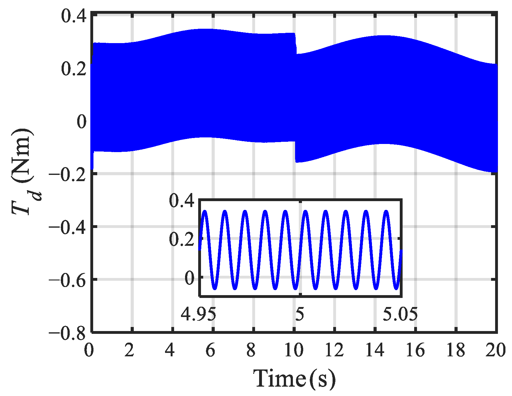
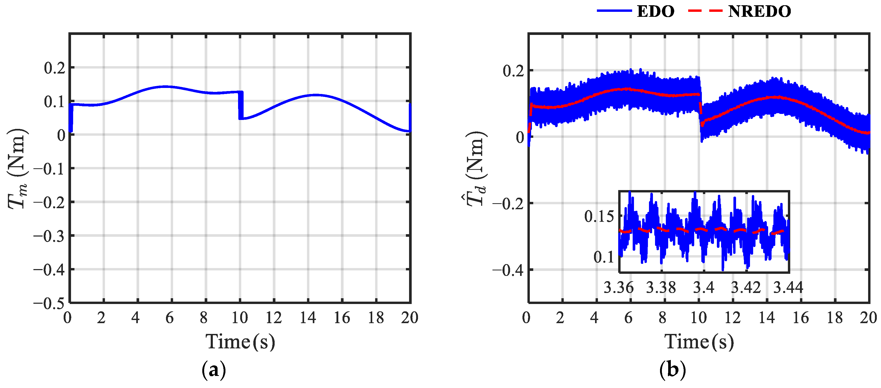
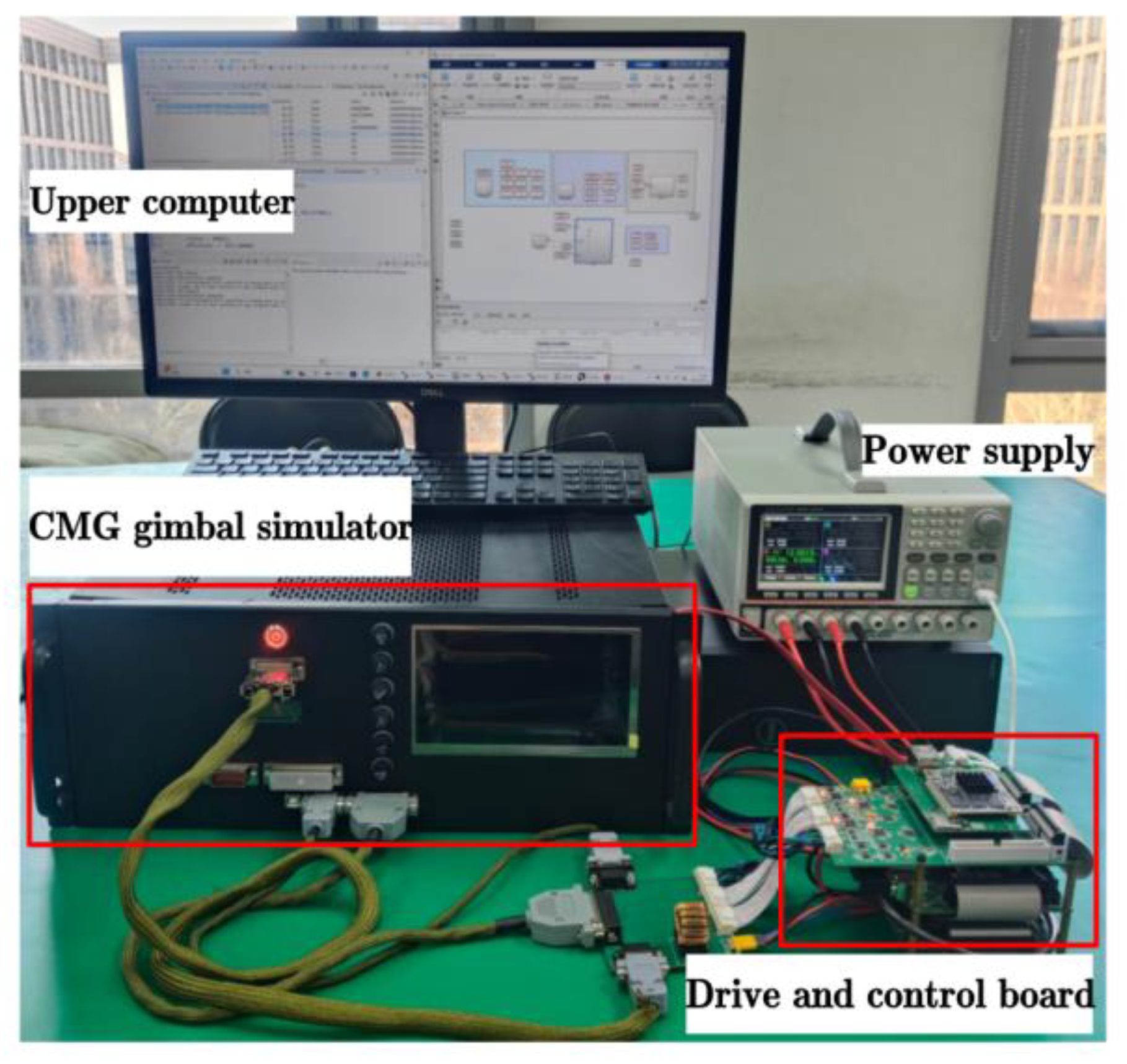
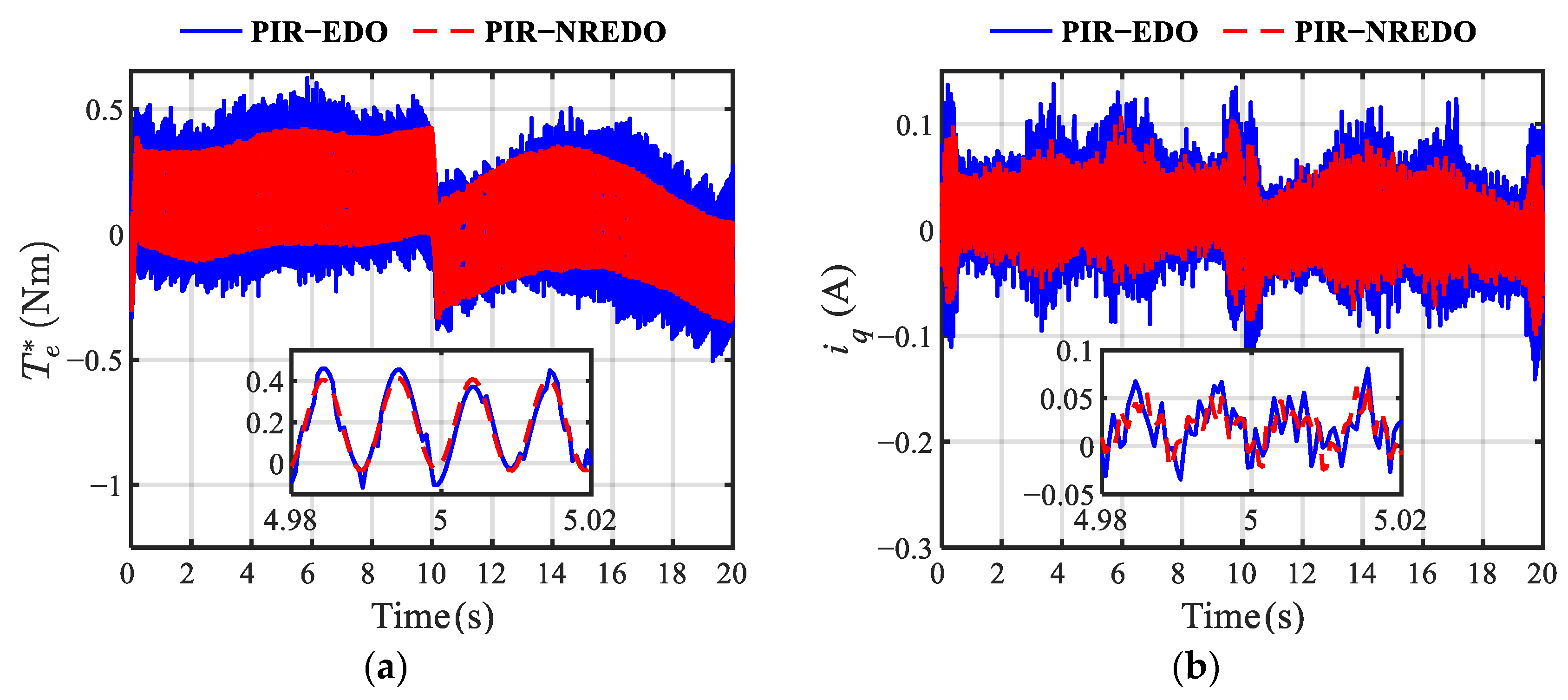
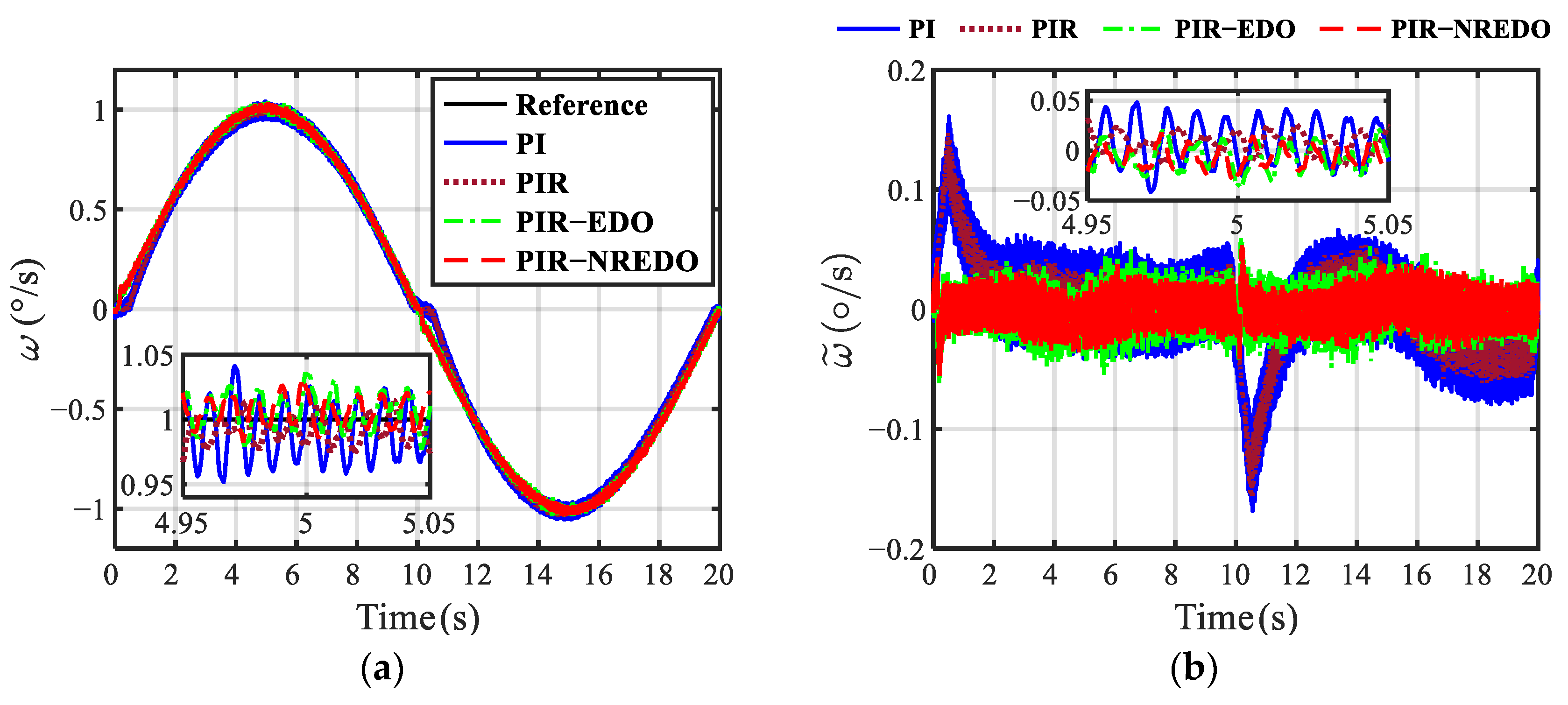
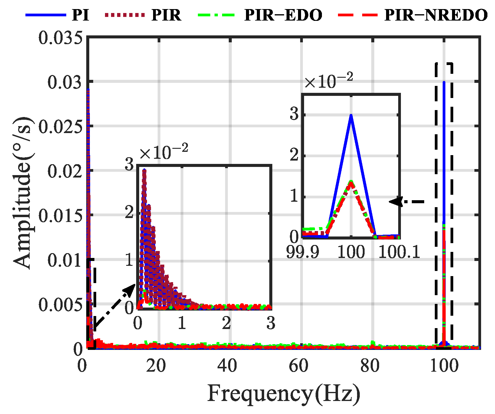
5. Experimental Results

In order to further verify the effectiveness of the proposed method, a semi-physical experiment was conducted. As shown in Figure 15, the experiment platform included a CMG gimbal simulator, a power supply, an upper computer, and a drive and control board.

The CMG gimbal simulator mainly has two advantages. First, the simulator can be utilized to simulate the mechanical and electrical characteristics of the real gimbal motor. Second, it is convenient to obtain the actual values of the disturbances and state parameters of the gimbal servo system compared with the real gimbal motor. Therefore, the performance of the proposed method could be conveniently evaluated by adopting the CMG gimbal simulator. Additionally, disturbance parameters could be directly set in real time via the upper computer during the experiment. Notably, the parameters of the gimbal servo system were the same as those in Table 2.

The digital signal processor used in the drive and control circuit was TMS320F28377D, with an execution period of 50 μs. As shown in Figure 1, an FOC-based control structure with the proposed method was adopted. The control period of the speed loop was 1 ms, and the control period of the current loop was 100μs. The disturbance parameters were set as shown in Table 3. The parameters of the speed controller in the experiment are as shown in

Table 5. The parameters of the speed controller in the experiment.

Parameters	${\mathit{K}}_{\mathit{p}}$	${\mathit{K}}_{\mathit{i}}$	${\mathit{K}}_{\mathit{r}}$	${\mathit{\varphi }}_{\mathit{r}}\left(°/\mathbf{s}\right)$	${\mathit{\omega }}_{\mathit{r}}(\mathbf{r}\mathbf{a}\mathbf{d}/\mathbf{s})$	${\mathit{\omega }}_{\mathit{o}}(\mathbf{r}\mathbf{a}\mathbf{d}/\mathbf{s})$
Values	10	10	200	250	$200\mathsf{\pi }$	$10\mathsf{\pi }$

. The desired speeds were the same as those in the simulation.

Case 1: Fixed Speed: The experiment curves at fixed speed are shown in Figure 16, Figure 17 and Figure 18. Figure 16 shows the estimation of $T_m$ by the EDO and NREDO. The disturbance estimation output of the EDO contains a significant amount of measurement noise. The measured gimbal angular speed used as the input to the observers contains significant measurement noise. However, the EDO does not take specific approaches to address this issue, resulting in decreased estimation accuracy. In contrast, the NREDO filters out most of the high-frequency noise through integral operations.

It can be observed from Figure 17a that the 100 Hz harmonic component in $T_e^{*}$ based on the PIR-NREDO maintains a better sinusoidal characteristic compared with the PIR-EDO. Due to the lower noise level in the NREDO, the waveform distortion in the q-axis current is also obviously reduced, as shown in Figure 17b.

As shown in Figure 18, the gimbal angular speed obtained when utilizing different control methods is presented. Obviously, the output of the speed controller based on the PIR-NREDO can maximize the suppression of multiple disturbances. Thus, the speed control performance is improved. The experimental results indicate that the PIR-NREDO can effectively suppress the effects of multiple disturbances and measurement noise. Therefore, the PIR-NREDO substantially improves the gimbal angular speed control accuracy.

Case 2: Sinusoidal Speed: The experiment curves at sinusoidal speed are presented in Figure 19, Figure 20, Figure 21 and Figure 22. As shown in Figure 19, the NREDO obviously decreases measurement noise in disturbance estimation. Thus, the torque ripple and current ripple are significantly reduced, as shown in Figure 20. This is substantially beneficial for the long-term operation of the gimbal motor. It can be observed from Figure 21 that the proposed method has superior speed control performance compared to other methods. In addition, the speed accuracy at the zero-crossing point is improved by utilizing the proposed method. The FFT results in Figure 22 indicate that the proposed method can suppress multiple disturbances simultaneously.

The gimbal angular speed RMSE in experiment is shown in

Table 6. Gimbal angular speed RMSE in experiment.

Methods		PI	PIR	PIR-EDO	PIR-NREDO
$\mathrm{RMSE}(°/\mathrm{s}$)	Case1	0.0338	0.0275	0.0135	0.0108
	Case2	0.0413	0.0373	0.0143	0.0124

. Due to non-ideal factors, such as current sampling errors and resolver measurement inaccuracies in the experiment, there is a certain amount of deviation between the accuracy of the experimental results and the simulation results. Compared with the PI controller, PIR controller, and PIR-EDO, the speed control accuracy based on the PIR-NREDO is improved by 68.05%, 60.73%, and 20% at fixed speed, respectively. At sinusoidal speed, the RMSE of the PIR-NREDO is reduced by 69.98%, 66.76%, and 13.29% in comparison with the PI controller, PIR controller, and PIR-EDO, respectively.

The numerical results in Section 4 and the experimental results in Section 5 indicate that the NREDO is superior to the EDO in measurement noise suppression, and the resonant controller can obviously reduce the high-frequency speed fluctuation caused by $T_r$. This demonstrates that the proposed method has significant application potential in practical scenarios.

6. Conclusions

To achieve high-precision speed control of CMG gimbal servo systems under multiple disturbances, a PIR-NREDO is proposed in this paper. Multiple disturbances are separated into the high-frequency periodic disturbance caused by rotor dynamic imbalance torque and other low-frequency disturbances. The NREDO is designed to estimate low-frequency disturbances. Notably, the NREDO more effectively balances disturbance estimation ability and measurement noise suppression ability, compared with an EDO. Subsequently, a resonant controller was utilized to suppress the high-frequency periodic disturbance. Compared with the PI controller, the PIR controller substantially enhanced the suppression of the 100 Hz periodic disturbance. The numerical simulation and experimental results demonstrate that the proposed method can significantly improve the speed control accuracy of CMG gimbal servo systems.

References

1. Li, H.; Wang, Y.; Han, B.; Chen, X. High-Precision Composite Control Based on Dual-Sampling-Rate Extended State Observer for Ultra-Low Speed Gimbal Servo System. IEEE J. Emerg. Sel. Top. Power Electron. 2022, 10, 5423–5434. [Google Scholar] [CrossRef]
2. Lu, M.; Hu, Y.; Wang, Y.; Li, G.; Wu, D.; Zhang, J. High Precision Control Design for SGCMG Gimbal Servo System. In Proceedings of the 2015 IEEE International Conference on Advanced Intelligent Mechatronics (AIM), Busan, Republic of Korea, 7–11 July 2015; pp. 518–523. [Google Scholar]
3. Luo, Q.; Li, D.; Zhou, W.; Jiang, J.; Yang, G.; Wei, X. Dynamic Modelling and Observation of Micro-Vibrations Generated by a Single Gimbal Control Moment Gyro. J. Sound Vib. 2013, 332, 4496–4516. [Google Scholar] [CrossRef]
4. Hekimoglu, B. Optimal Tuning of Fractional Order PID Controller for DC Motor Speed Control via Chaotic Atom Search Optimization Algorithm. IEEE Access 2019, 7, 38100–38114. [Google Scholar] [CrossRef]
5. Kelly, R.; Moreno, J. Learning PID Structures in an Introductory Course of Automatic Control. IEEE Trans. Educ. 2001, 44, 373–376. [Google Scholar] [CrossRef]
6. Shin, H.-B.; Park, J.-G. Anti-Windup PID Controller with Integral State Predictor for Variable-Speed Motor Drives. IEEE Trans. Ind. Electron. 2012, 59, 1509–1516. [Google Scholar] [CrossRef]
7. Tang, K.S.; Man, K.F.; Chen, G.; Kwong, S. An Optimal Fuzzy PID Controller. IEEE Trans. Ind. Electron. 2001, 48, 757–765. [Google Scholar] [CrossRef]
8. Hong, Y.; Yao, B. A Globally Stable High-Performance Adaptive Robust Control Algorithm with Input Saturation for Precision Motion Control of Linear Motor Drive Systems. IEEE/ASME Trans. Mechatron. 2007, 12, 198–207. [Google Scholar] [CrossRef]
9. Valente, G.; Formentini, A.; Papini, L.; Gerada, C.; Zanchetta, P. Performance Improvement of Bearingless Multisector PMSM With Optimal Robust Position Control. IEEE Trans. Power Electron. 2019, 34, 3575–3585. [Google Scholar] [CrossRef]
10. Mendoza-Mondragon, F.; Hernandez-Guzman, V.M.; Rodriguez-Resendiz, J. Robust Speed Control of Permanent Magnet Synchronous Motors Using Two-Degrees-of-Freedom Control. IEEE Trans. Ind. Electron. 2018, 65, 6099–6108. [Google Scholar] [CrossRef]
11. Xu, S.; Wu, Z. Adaptive Learning Control of Robot Manipulators via Incremental Hybrid Neural Network. Neurocomputing 2024, 568, 127045. [Google Scholar] [CrossRef]
12. Li, X.; Li, S. Speed Control for a PMSM Servo System Using Model Reference Adaptive Control and an Extended State Observer. J. Power Electron. 2014, 14, 549–563. [Google Scholar] [CrossRef]
13. Yin, Y.; Liu, L.; Vazquez, S.; Xu, R.; Dong, Z.; Liu, J.; Leon, J.I.; Wu, L.; Franquelo, L.G. Disturbance and Uncertainty Attenuation for Speed Regulation of PMSM Servo System Using Adaptive Optimal Control Strategy. IEEE Trans. Transp. Electrific. 2023, 9, 3410–3420. [Google Scholar] [CrossRef]
14. Choi, H.H.; Leu, V.Q.; Choi, Y.-S.; Jung, J.-W. Adaptive Speed Controller Design for a Permanent Magnet Synchronous Motor. IET Electr. Power Appl. 2011, 5, 457. [Google Scholar] [CrossRef]
15. Comanescu, M.; Xu, L.; Batzel, T.D. Decoupled Current Control of Sensorless Induction-Motor Drives by Integral Sliding Mode. IEEE Trans. Ind. Electron. 2008, 55, 3836–3845. [Google Scholar] [CrossRef]
16. Li, S.; Zhou, M.; Yu, X. Design and Implementation of Terminal Sliding Mode Control Method for PMSM Speed Regulation System. IEEE Trans. Ind. Inf. 2013, 9, 1879–1891. [Google Scholar] [CrossRef]
17. Lu, H.; Yang, D.; Su, Z. Improved Sliding Mode Control for Permanent Magnet Synchronous Motor Servo System. IET Power Electron. 2023, 16, 169–179. [Google Scholar] [CrossRef]
18. Yepes, A.G.; Freijedo, F.D.; Lopez, O.; Doval-Gandoy, J. Analysis and Design of Resonant Current Controllers for Voltage-Source Converters by Means of Nyquist Diagrams and Sensitivity Function. IEEE Trans. Ind. Electron. 2011, 58, 5231–5250. [Google Scholar] [CrossRef]
19. Xia, C.; Ji, B.; Yan, Y. Smooth Speed Control for Low-Speed High-Torque Permanent-Magnet Synchronous Motor Using Proportional–Integral–Resonant Controller. IEEE Trans. Ind. Electron. 2015, 62, 2123–2134. [Google Scholar] [CrossRef]
20. Hu, M.; Hua, W.; Ma, G.; Xu, S.; Zeng, W. Improved Current Dynamics of Proportional-Integral-Resonant Controller for a Dual Three-Phase FSPM Machine. IEEE Trans. Ind. Electron. 2021, 68, 11719–11730. [Google Scholar] [CrossRef]
21. Tian, M.; Wang, B.; Yu, Y.; Dong, Q.; Xu, D. Robust Adaptive Resonant Controller for PMSM Speed Regulation Considering Uncertain Periodic and Aperiodic Disturbances. IEEE Trans. Ind. Electron. 2023, 70, 3362–3372. [Google Scholar] [CrossRef]
22. Kim, K.-S.; Rew, K.-H.; Kim, S. Disturbance Observer for Estimating Higher Order Disturbances in Time Series Expansion. IEEE Trans. Autom. Control 2010, 55, 1905–1911. [Google Scholar] [CrossRef]
23. Yan, R.; Wu, Z. Attitude Stabilization of Flexible Spacecrafts via Extended Disturbance Observer Based Controller. Acta Astronaut. 2017, 133, 73–80. [Google Scholar] [CrossRef]
24. He, T.; Wu, Z. Extended Disturbance Observer with Measurement Noise Reduction for Spacecraft Attitude Stabilization. IEEE Access 2019, 7, 66137–66147. [Google Scholar] [CrossRef]
25. Zhang, Y.; Wu, Z.; Wei, T. Aerodynamic Disturbance Estimation in Quadrotor Landing on Moving Platform via Noise Reduction Extended Disturbance Observer. IEEE Sens. J. 2024, 24, 37566–37574. [Google Scholar] [CrossRef]
26. Jiang, Y.; Yang, J.; Li, S. Multi-Frequency-Band Uncertainties Rejection Control of Flexible Gimbal Servo Systems via a Comprehensive Disturbance Observer. IEEE Trans. Circuits Syst. I 2023, 71, 794–804. [Google Scholar] [CrossRef]
27. Wang, C.; Peng, J.; Pan, J. A Novel Friction Compensation Method Based on Stribeck Model with Fuzzy Filter for PMSM Servo Systems. IEEE Trans. Ind. Electron. 2023, 70, 12124–12133. [Google Scholar] [CrossRef]
28. Fei, Q.; Deng, Y.; Li, H.; Liu, J.; Shao, M. Speed Ripple Minimization of Permanent Magnet Synchronous Motor Based on Model Predictive and Iterative Learning Controls. IEEE Access 2019, 7, 31791–31800. [Google Scholar] [CrossRef]
29. Huang, L.; Wu, Z.; Wang, K. High-Precision Anti-Disturbance Gimbal Servo Control for Control Moment Gyroscopes via an Extended Harmonic Disturbance Observer. IEEE Access 2018, 6, 66336–66349. [Google Scholar] [CrossRef]
30. Cui, Y.; Yang, Y.; Zhao, L.; Zhu, Y.; Qiao, J.; Guo, L. Composite Control for Gimbal Systems with Multiple Disturbances: Analysis, Design, and Experiment. IEEE Trans. Syst. Man Cybern Syst. 2023, 53, 4789–4798. [Google Scholar] [CrossRef]
31. Analog Devices. Available online: https://www.analog.com/media/en/technical-documentation/data-sheets/ad2s1210.pdf (accessed on 12 March 2025).
Figure 1. The structure of the system under the proposed method.
Actuators 14 00196 g001
Figure 2. Amplitude–frequency characteristic curves of a 3rd-order and 4th-order EDO and NREDO: (a) disturbance estimation ability; (b) noise suppression ability.
Actuators 14 00196 g002
Figure 3. A Bode diagram of the closed-loop system by utilizing PI and PIR.
Actuators 14 00196 g003
Figure 4. A simplified block diagram of the control system.
Actuators 14 00196 g004
Figure 5. The Nyquist diagram of the open-loop transfer function G o ( s ) .
Actuators 14 00196 g005
Figure 6. Simulation curve of T d at fixed speed.
Actuators 14 00196 g006
Figure 7. Simulation curves of T m and disturbance estimation under EDO and NREDO at fixed speed: (a) T m ; (b) T ^ d .
Actuators 14 00196 g007
Figure 8. Simulation curves of desired electromagnetic torque T e * and q-axis current i q under PIR-EDO and PIR-NREDO at fixed speed: (a) T e * ; (b) i q .
Actuators 14 00196 g008
Figure 9. Simulation curves of gimbal angular speed at fixed speed: (a) gimbal angular speed; (b) FFT results of gimbal angular speed.
Actuators 14 00196 g009
Figure 10. Simulation curve of T d at sinusoidal speed.
Actuators 14 00196 g010
Figure 11. Simulation curves of T m and disturbance estimation under EDO and NREDO at sinusoidal speed: (a) T m ; (b) T ^ d .
Actuators 14 00196 g011
Figure 12. Simulation curves of desired electromagnetic torque T e * and q-axis current i q under PIR-EDO and PIR-NREDO at sinusoidal speed: (a) T e * ; (b) i q .
Actuators 14 00196 g012
Figure 13. Simulation curves of gimbal angular speed at sinusoidal speed: (a) gimbal angular speed; (b) gimbal angular speed errors.
Actuators 14 00196 g013
Figure 14. Simulation curves of FFT results of gimbal angular speed at sinusoidal speed.
Actuators 14 00196 g014
Figure 15. Experiment platform.
Actuators 14 00196 g015
Figure 16. Experiment curves of T m and disturbance estimation under EDO and NREDO at fixed speed: (a) T m ; (b) T ^ d .
Actuators 14 00196 g016
Figure 17. Experiment curves of desired electromagnetic torque T e * and q-axis current i q under PIR-EDO and PIR-NREDO at fixed speed: (a) T e * ; (b) i q .
Actuators 14 00196 g017
Figure 18. Experiment curves of gimbal angular speed at fixed speed: (a) gimbal angular speed; (b) FFT of gimbal angular speed.
Actuators 14 00196 g018
Figure 19. Experiment curves of T m and disturbance estimation under EDO and NREDO at sinusoidal speed: (a) T m ; (b) T ^ d .
Actuators 14 00196 g019
Figure 20. Experiment curves of desired electromagnetic torque T e * and q-axis current i q under PIR-EDO and PIR-NREDO at sinusoidal speed: (a) T e * ; (b) i q .
Actuators 14 00196 g020
Figure 21. Experiment curves of gimbal angular speed at sinusoidal speed: (a) gimbal angular speed; (b) gimbal angular speed errors.
Actuators 14 00196 g021
Figure 22. Experiment curves of FFT results of gimbal angular speed at sinusoidal speed.
Actuators 14 00196 g022