Abstract
In an intelligent driving system, the rationality of driving decisions and the trajectory planning scheme directly determines the safety and stability of the system. Existing research mostly relies on high-definition maps and empirical parameters to estimate road adhesion conditions, ignoring the direct impact of real-time road status changes on the dynamic feasible domain of vehicles. This paper proposes an intelligent driving decision-making and trajectory planning method that comprehensively considers the influence factors of vehicle–road interaction. Firstly, real-time estimation of road adhesion coefficients was achieved based on the recursive least squares method, and a dynamic adhesion perception mechanism was constructed to guide the decision-making module to restrict lateral maneuvering behavior under low-adhesion conditions. A multi-objective lane evaluation function was designed for adaptive lane decision-making. Secondly, a longitudinal and lateral coupled trajectory planning framework was constructed based on the traditional lattice method to achieve smooth switching between lateral trajectory planning and longitudinal speed planning. The planned path is tracked based on a model predictive control algorithm and dual PID algorithm. Finally, the proposed method was verified on a co-simulation platform. The results show that this method has good safety, adaptability, and control stability in complex environments and dynamic adhesion conditions.
1. Introduction
An autonomous driving system typically consists of four basic modules: perception, decision-making, planning, and control. Driving decisions and trajectory planning are the key bridge connecting perception and execution control [1]. Road conditions, lane infrastructure, and surrounding vehicles influence the process of vehicle driving decisions and trajectory planning [2]. Road friction, damage, or water accumulation limit the available adhesion, affecting braking and acceleration strategies. Lane width, marking, and guardrail deformation define lateral driving space, left and right lane changes, and obstacle avoidance feasibility, and the speed and intention of the surrounding vehicles form a dynamic constraint, which prompts the system to switch between lane keeping, overtaking, or longitudinal driving in real time. The decision-making and trajectory planning module must integrate this information to generate an executable path that is both safe, compliant, efficient, and smooth [3]. Most current research obtains accurate road layout and lane infrastructure information through high-definition maps and self-positioning, and acquires dynamic obstacle information through onboard sensors [4]. At the same time, it assumes that road adhesion conditions ( the tire–road friction coefficient) can be provided by high-definition maps or empirical values [5], while ignoring the direct impact of real-time road changes (snow accumulation, water accumulation, wear, etc.) on the vehicle’s dynamic limits and safety indicators [6]. In fact, the road adhesion coefficient determines the maximum force that the tire can exert during acceleration, braking, and steering. If the adhesion coefficient is overestimated, it may cause the control system to request excessive power output, leading to tire slipping, skidding, and even vehicle loss of control. If the estimated value is too conservative, it will limit the vehicle’s dynamic performance and reduce traffic efficiency and maneuverability [7]. Therefore, considering real-time road changes at the front end of the planning–control link and designing a reasonable and efficient driving decision mechanism can help vehicles reasonably plan a driving path in highly dynamic scenarios such as emergency braking, obstacle avoidance, lane changing, and high-speed steering, and ensure that the motion control strategy is safely and effectively executed. This is of great significance for improving the safety, comfort, and traffic efficiency of intelligent vehicles in complex environments [8,9].
Current methods for estimating road adhesion coefficients can be classified into those based on causes, effects, and data-driven and hybrid approaches [10]. Effect-based methods typically establish the longitudinal and lateral dynamics of the vehicle and design filters or observers to measure and analyze the vehicle response caused by road changes to estimate the road adhesion coefficient [11,12]. This method does not require expensive sensor equipment and has better real-time performance and higher accuracy compared to other methods. It is widely used in vehicles [13,14]. An expectation maximization robust extended Kalman filter, which considers the influence of sensor data loss on the estimation accuracy of sideslip angle, yaw rate and vehicle speed, was proposed by Wang [15]. A method based on model learning, combined with an event-triggered cubature Kalman filter and extended Kalman neural network, was proposed by Wang to identify the road adhesion coefficient [16]. Liu proposed a method for estimating vehicle state parameters and road adhesion coefficients by integrating sliding mode theory, trigonometric function group fitting, and cubic spline interpolation within an extended Kalman filter framework [17]. A strong tracking unscented Kalman filtering method [18] with faster convergence speed and ability to dynamically estimate the road adhesion coefficient on time-varying roads was designed by Ping. RLS is one of the effect-based methods, converting the complex nonlinear adhesion coefficient estimation of the vehicle into a linear model parameter tracking problem [19]. It achieves efficient calculation and real-time updates through recursive characteristics and adapts to sudden road changes through forgetting factors. Compared to traditional offline algorithms or complex nonlinear methods such as Kalman filtering, the RLS method demonstrates strong practical value on resource-constrained on-board ECUs [20]. The least squares method was employed by Chen to perform multivariate fitting on the relationship curve between slip rate and adhesion coefficient, thereby estimating the road status [21]. A three-dimensional mapping model of slip rate, road adhesion coefficient, and road peak adhesion coefficient was established by He, and the road status was estimated based on the slope of the curve of the surface model [22].
Recently, research on intelligent vehicle driving decision-making has been evolving from rule-driven to data-driven game decision-making, with the core being to achieve multi-objective dynamic balance within a safety framework [23]. A driving operation diagram was utilized by Zhang to implicitly represent the driving styles of a self–driving vehicle and other vehicles. Through supervised learning, decision-making strategies were learned from human driving data and rule-based indicators were explicitly introduced to achieve adaptive lane-changing decisions based on driving styles [24]. Yang proposed a human–machine collaborative continuous learning framework. The driver provided demonstration data through the takeover mechanism, dynamically corrected the AV’s decision deviations, designed an anti-forgetting learning algorithm, and combined behavior cloning with Q-value optimization to generate personalized strategies [25]. Trajectory planning research has evolved multiple technical routes at “global–local” levels: traditional graph search, sampling-, optimization-, and learning-based methods [26,27]. The traditional graph search method demonstrates stability in structured environments due to its determinism and explainability, making it suitable for global path planning. However, when dealing with dynamic obstacles, unstructured roads, or uncertain behaviors of traffic participants, its adaptability is poor [28]. The sampling-based method, relying on the discretization approach, quickly forms in unknown environments, but has the bottleneck of rough trajectories and inability to meet vehicle kinematic constraints [29] directly. The optimization-based method obtains smooth trajectories and differentiable control instructions through continuous optimization. However, it is prone to falling into computational bottlenecks or local optima when the obstacle complexity or search space dimensionality is high [30]. To balance the efficiency of discrete search and the feasibility of continuous optimization, the academic community proposed the state lattice trajectory planning: first, design offline a set of motion primitives that comply with vehicle kinematics and form a “gridded” state lattice in the pose space, then use online heuristic searching to concatenate the primitives between grid points to generate a fully dynamic and feasible trajectory [31]. The lattice method benefits from its prior kinematic feasibility, discrete search convergence, real-time heuristic cost, offline optimization for comfort, and easy integration with vehicle dynamic models and constraints, and has become the mainstream solution in scenarios such as highway lane changing, urban road overtaking, and multi-vehicle formation, which combines real-time performance and trajectory quality [32]. Currently, the lattice method mainly performs a gridded search in the lateral direction. It is often used for lateral trajectory planning, ignoring the dynamic coupling effect of the longitudinal dimension in the trajectory generation process. In complex dynamic environments such as variable obstacle avoidance, emergency braking, or low-adhesion road surfaces, the longitudinal behavior is closely coupled with the lateral path, and relying solely on lateral search makes it difficult to exactly reflect overall dynamic feasibility and safety [33]. To address this issue, this paper improves the lattice method.
The primary innovations of this paper are:
- In the motion decision and trajectory planning module, the influence of road conditions (adhesion coefficient, curvature) is considered to improve the safety of the autonomous driving system.
- A longitudinal and lateral coupled lattice trajectory planning method is proposed, which can improve the dynamic feasibility of the trajectory and ensure longitudinal–lateral consistency under complex working conditions.
The rest of this article is arranged as follows. In the Section 2, the overall research framework of this article is introduced. In the Section 3, vehicle–road comprehensive influencing factors are considered to aid in designing the vehicle driving decision mechanism. In the Section 4, the lattice method is improved, the longitudinal and lateral coupled trajectory planning algorithm for vehicles is studied, and the trajectory tracking module is constructed to achieve intelligent vehicle motion control. In the Section 5, Simulink–CarSim–Prescan joint simulation verification is carried out. In the Section 6, the entire article is summarized and future work is presented.
2. Overall Research Framework
This paper proposes a driving decision-making and trajectory planning framework that comprehensively considers the influencing factors of vehicles and roads, as shown in Figure 1. Firstly, in the environmental perception stage, the longitudinal adhesion coefficient of the road surface represents the maximum longitudinal traction/braking force capability that the tires can provide under the current road conditions, and is one of the basic parameters for the safety and stability control of intelligent vehicles. This paper utilizes the RLS method to estimate the longitudinal road status in real time and with high accuracy. It combines onboard sensors to gather information on surrounding obstacles, thereby providing environmental perception information that supports subsequent system safety feasibility judgments, path and strategy optimization, and other related tasks. Secondly, in the motion decision-making stage, vehicle behavior decisions are made based on road adhesion conditions and a lane weighting function reflecting the feasibility and risk level of the lane is designed, thereby constructing a driving decision-making mechanism that comprehensively considers the influence factors of vehicles and roads. In the trajectory planning and motion control stage, a longitudinal and lateral coupled trajectory planning algorithm based on lattice is developed. Longitudinal speed planning and lateral trajectory planning are carried out according to the decision results, and smooth switching between the two is achieved. Combined with model predictive control (MPC) and dual PID control algorithms, the intelligent vehicle can achieve precise trajectory tracking and stable control in complex scenarios. The algorithm is simulated and verified on a horizontal structured road, and the influence of road slope is not considered. The proposed decision-making and planning framework for autonomous driving vehicles effectively enhances the system’s adaptability to complex dynamic environments, realizes robust planning and control in low-adhesion and high-interference scenarios, significantly improves the rationality of vehicle system decision-making, trajectory feasibility, and operational safety, and lays a foundation for the practical deployment of autonomous driving systems.
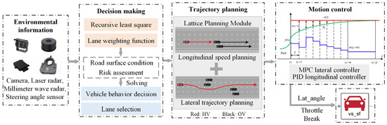
Figure 1.
Overall research framework.
3. Vehicle Driving Decision-Making Mechanism Considering the Comprehensive Impact of Vehicles and Roads
3.1. Estimation of Longitudinal Road Adhesion Coefficient Based on RLS
To obtain a real-time and accurate estimate of the longitudinal pavement adhesion coefficient and to support the subsequent development of the vehicle’s longitudinal and lateral motion controllers, this chapter constructs a two-degree-of-freedom vehicle dynamic model. A tire mechanical model combining a linear region and saturation region is used, with an emphasis on the relationship between longitudinal force and slip rate.
Establish the vehicle dynamic model:
The conversion relationship between the resultant force acting on the tire in the longitudinal and lateral directions and the actual lateral force and longitudinal force exerted on the tire is as follows:
where is the curb weight, is the longitudinal acceleration, is the lateral acceleration, is the rotational inertia of the vehicle around the z-axis, is the rotation angle of the front wheels, is the roll angle, is the roll angular velocity, is the camber angle of the center of gravity, is the camber angle of the front wheels, is the camber angle of the rear wheels, is the speed of the front wheels, is the speed of the rear wheels, are the forces exerted by the front and rear wheels in the x-axis direction, are the forces exerted by the front and rear wheels in the y-axis direction, are the longitudinal forces exerted by the front and rear wheels of the vehicle, are the lateral forces exerted by the front and rear wheels of the vehicle, is the distance from the center of gravity to the front axle, and is the distance from the center of gravity to the rear axle.
The lateral and longitudinal velocities of the vehicle have different expressions in the vehicle body coordinate system and the earth coordinate system. The conversion relationship between the two can be expressed as:
Whole-vehicle longitudinal dynamic model:
where represent the rotational inertia of the front and rear wheels, is the gravitational acceleration, is the longitudinal acceleration of the vehicle, is the rolling radius of the wheel, is the road adhesion coefficient, is the air resistance coefficient, is the frontal area, is the air density, is the driving torque, and is the braking torque, .
Braking or driving force of the front and rear axles of the vehicle:
where represents the road adhesion coefficient, is an empirical constant, and is the longitudinal slip rate of the wheel.
Slip ratio during vehicle acceleration/deceleration:
where represents the radius of the wheel, while (wheel speed) and (vehicle speed) are known quantities.
From the wheel rotation dynamic equation:
where represents the braking or driving torque of the wheels and is the coefficient of rolling resistance of the wheels.
When a vehicle is accelerating or braking, the acceleration is constrained by the road status, with the relationship being . Within a small slip rate range, there is approximately a direct proportional relationship between the adhesion coefficient and the slip rate:
where is the slope, is the longitudinal force of the tire, and is the vertical force of the tire. In the small slip rate range, the reaction force of the ground on the driving wheel can approximately represent the longitudinal force of the tire .
Transform it into the recursive least squares method expression:
where .
where represents the maximum slip rate within the linear region, and p is the proportion coefficient of the maximum road adhesion coefficient within the linear region to the peak road adhesion coefficient. The derivation process of the longitudinal road adhesion coefficient estimation algorithm based on the RLS method is as shown in Algorithm 1.
| Algorithm 1. RLS method |
| Input: the braking or driving force , the longitudinal acceleration , the adhesion coefficient at the previous moment , the covariance matrix at previous time |
| Output: the adhesion coefficient at the current moment , the covariance matrix at current time |
|
3.2. Intelligent Vehicle Driving Decision Mechanism Considering the Comprehensive Impact of Vehicles and Road Surfaces
To enhance the dynamic adaptability of the autonomous driving system in complex environments, this paper proposes a driving decision-making mechanism that integrates dynamic vehicle–road information, aiming to ensure driving safety and adaptability under different adhesion conditions and traffic flow distributions.
Based on the real-time estimation method of the road adhesion coefficient proposed in Section 3.1, the current road adhesion capacity is characterized by the estimated value . The maximum lateral acceleration that the vehicle can withstand is approximately . According to the ISO 3888-1 double-lane-change test [34], it is indicated that during the period when the risk of vehicle skidding and rollover during lane changing is higher, resulting in lane change-related accidents accounting for more than 17% of all accidents in icy and snowy weather. Based on the above risk trend, driving behavior decision-making for low-adhesion road surfaces is designed:
where is the curvature coefficient. During the simulation process, when the penalty for the low-adhesion section is insufficient, resulting in a low lane-changing success rate and an increased risk of vehicle skidding. When overly conservative behavior occurs, leading to a decrease in lane-changing efficiency. Therefore, in this framework, to ensure successful lane changes while also paying attention to lane-changing efficiency. ensures that the current lane is not penalized. This switching mechanism ensures that the vehicle can dynamically adjust its operational capability boundaries according to the actual ground conditions.
Normalized processing, attachment condition evaluation function:
Under the longitudinal and lateral coupling planning mode, the system further takes into account the current road traffic scene information of the vehicle, comprehensively perceives the obstacle status and traffic flow speed distribution of each lane around the vehicle, and conducts dynamic assessment of the available lanes. The current lane of the HV is defined as and a lane set is constructed within the lane expansion range . For each candidate lane, the comprehensive evaluation function is constructed as:
where represents the forward available distance of the HV on this lane, reflecting the spatial smoothness of the lane. represents the deviation between the target vehicle speed and the HV’s expected speed, measuring the potential following efficiency. represents the potential risk estimation of this lane, taking into account obstacle density, the behavior of the preceding vehicle changing lanes, and interference from adjacent lanes. represents the road adhesion condition score. The lower the adhesion coefficient, the greater the penalty. represents the curvature of the road, avoiding the choice of a fast-turning lane and improving stability and safety.
where represents the vertical distance between the obstacle vehicle and the self-vehicle and is the sensor’s line of sight distance, which is set at 50 m:
where represents the speed of the vehicle itself, while represents the speed of the vehicle immediately in front. When the speed difference is greater than 0, the speed is reduced.
The risk function is used to quantify the probability that a vehicle will encounter potential conflicts, collisions, or dynamic disturbances after entering the candidate lane . It is the core quantity for safety assessment in the decision-making module and is divided into the following key components:
where represents the static obstacle risk term, indicating the density and distance of fixed obstacles on lane is the dynamic risk term, reflecting the potential interference that other dynamic vehicles in the lane may cause to this vehicle, such as relative speed, relative position, and lane-changing tendency, and is used to represent the uncertain term, reflecting the possible errors in the perception system [35].
In the comprehensive evaluation function, are weight factors. The adaptive adjustment strategy for the weight factors is as follows:
Establish the security level of the scene:
where represents the road adhesion coefficient, represents the curvature information, is a constant term, and indicates selecting the median value within the parentheses. Through the construction of the scene safety degree, in slippery/sudden turns/high-speed conditions, is close to 1, and the selection of the weight factor leans more towards safety, while in straight roads/dry conditions/low-speed conditions, is close to 0 and the selection of the weight factor leans more towards efficiency.
where represents the security weight vector and represents the efficiency weight vector. The sizes of the corresponding elements of in the vectors are determined through parameter adjustment. Each vector contains elements.
The system selects the lane that maximizes the benefit for each candidate lane as the current optimal driving lane:
The decision-making module outputs specific behavior instructions based on the selected optimal lane and calls the trajectory planner to generate dynamic trajectories, ensuring adaptive, robust, and efficient autonomous driving behavior in real-time changing road and traffic conditions.
4. Coupled Longitudinal and Lateral Trajectory Planning of Vehicles Based on the Lattice Method
This paper improves the traditional lattice method and designs a trajectory planning framework with both longitudinal and lateral coupling capabilities. This method can dynamically switch between joint longitudinal and lateral trajectory planning and the single longitudinal planning mode based on the behavioral instructions issued by the upper-level decision module and the current environmental perception results. It enables a smooth transition between lateral trajectory planning and longitudinal speed planning, enhancing the consistency and robustness of the decision-making and planning in complex scenarios such as slippery roads and dense obstacles. The key variables in the planning algorithm are summarized as Table 1.

Table 1.
Main parameters of the planning algorithm.
4.1. Coordinate Transformation
In intelligent vehicle trajectory planning and control, the Frenet coordinate system is based on the reference line and represents the vehicle position as the arc length along the path direction and the lateral offset which can effectively simplify the trajectory generation problem and make the planning more efficient and compliant with road constraints [36]. The Cartesian coordinate system reflects the actual position of the vehicle in the global environment and is necessary for perception data processing, map interaction, and control execution. The conversion between the two coordinate systems is shown in Figure 2. During the planning process, global coordinate systems are constructed to record road information, including lanes and road curvatures, and a global reference path is generated, as shown in Figure 3.
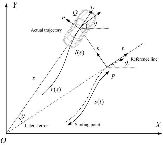
Figure 2.
Coordinate system transformation diagram.
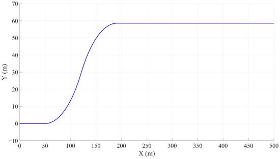
Figure 3.
Global reference path.
According to Figure 2, the position coordinates of the vehicle at the current moment are:
where represents the position vector of the HV, represents the point obtained by projecting the vehicle onto the reference line, is the curve distance from the starting point to point represents the position vector of the vehicle on the reference line, and represents the normal unit vector at point .
After conversion, the vehicle motion state is represented as while in the Frenet system, it is expressed as represents the heading angle, represents the curvature in the current state, represents the vehicle speed, and represents the acceleration. represent the derivatives of the lateral displacement with respect to time, and represent the derivatives of the lateral displacement with respect to the longitudinal displacement. is the distance between adjacent points.
The tangential and normal unit vectors at the projection point of the vehicle position on the reference line are expressed as:
Course angle and curvature calculation:
The conversion relationship between the two coordinate systems is summarized as follows.
- Conversion from Cartesian coordinate system to Frenet coordinate system:
- Conversion from Frenet coordinate system to Cartesian coordinate system:
4.2. Lateral Trajectory Planning
In order to take into account the feasibility of the path and the smoothness of the trajectory, this paper adopts a two-stage trajectory generation structure combining dynamic programming (DP) and quadratic programming (QP), conducting path search and trajectory optimization separately. This achieves a balance between search efficiency and trajectory quality. Firstly, from the obstacle information in the global coordinate system, obstacles existing in the forward field of view and the lateral perceptible area are selected. The obstacle information is classified and the static obstacle position, dynamic obstacle position, and velocity vector are output, which are used as input for local path planning. The position vector and longitudinal–lateral relative distance of the obstacle relative to the host vehicle are calculated:
For the square of the distance between each obstacle point and each trajectory point:
Based on the starting position of the vehicle and the position of static obstacles, a dynamic programming method is used to search for a lateral trajectory path with the minimum cost within the prescribed lateral grid, and the sequence of the optimal trajectory is output. A quintic polynomial trajectory function is constructed, with the initial state and the target state . For the lateral motion of the vehicle:
Derivation:
Matrix form:
When :
When :
where coefficient vector is obtained by solving the system of equations.
Separately construct the trajectory smoothing cost term and the obstacle avoidance cost term:
where are weighting coefficients, is the Euclidean distance between the vehicle trajectory point and the obstruction, is the set collision penalty coefficient, indicating a strong penalty, and serves as a progressive penalty function, with a closer distance resulting in a greater cost. By constructing a trajectory smoothness cost term and an obstacle avoidance cost term, the degree of fluctuation of the trajectory is minimized, preventing the trajectory from approaching or crossing the obstacle and achieving a balance between safety and feasibility during driving.
In order to further enhance the continuity and dynamic controllability of the trajectory, this paper introduces a quadratic programming optimization module based on the DP dynamic programming path. The QP module takes the output of DP as the reference path, constructs a cubic derivative smoothing objective function, optimizes the lateral offset of the vehicle and its first-order, second-order, and third-order derivative terms, and optimizes the variable vector:
The cost function is defined as follows:
where is a symmetric positive definite cost weight matrix, including the centerline deviation cost the lateral velocity penalty term the lateral acceleration penalty term and the jerk penalty term (rate of change of acceleration) is a linear term.
Establishing dynamic continuity constraints:
Establishing constraints on the variation range of derivatives:
Establishing the lateral boundary of the obstacle, taking into account the vehicle width and the offset positions of the front axles:
4.3. Longitudinal Speed Planning
To achieve the integration and smooth transition of lateral trajectory planning and longitudinal speed planning, in this section, the longitudinal speed distribution is optimized and designed, and the longitudinal speed is independently planned to generate a complete time sequence trajectory. Given the position sequence under the reference line, continuous curves for time parameter speed and acceleration are generated to realize the integration from a spatial trajectory to a spatial–temporal trajectory.
Establish boundary conditions:
Based on the integral constraints of first-order and second-order derivatives, the continuity of the vehicle’s position and velocity and acceleration are ensured at each time period:
Based on the end position of the dynamic planning path and the recommended planning duration an initial longitudinal velocity trajectory consisting of three dimensions—position, speed, and acceleration—is constructed. A minimum jerk trajectory optimization model with position constraints, speed limits, and acceleration constraints is adopted, and the objective function is:
where represents the acceleration at the moment, the second term constrains the jerk smoothness, and is the weighting coefficient.
Using as the index, interpolate the lateral trajectory as the function . According to the Frenet transformation formula, restore it to the Cartesian trajectory and generate the final complete trajectory . Finally, concatenate the current frame’s trajectory with the remaining trajectory from the previous frame to construct a complete prediction trajectory queue, ensuring smoothness, continuity, and control tracking performance of the trajectory.
4.4. Trajectory Tracking
In this paper, the MPC algorithm is employed to achieve high-precision lateral trajectory control for vehicles. By optimizing the vehicle’s future short-term motion trajectory in real time, considering vehicle dynamic constraints and road boundary conditions, it effectively improves the path tracking accuracy and stability of the vehicle in complex conditions such as cornering and lane changing. The vehicle dynamic prediction model is as follows:
where represents the quantity of state, represents the control input, and represent the system matrices obtained through the linearization of vehicle dynamics.
MPC cost function:
where represents the length of the prediction time domain, represents the length of the control time domain, and represent the weight matrices, which are used to balance the trajectory error and the smoothness of the control input.
In longitudinal trajectory tracking, a dual-closed-loop PID control strategy based on position loop and speed loop is designed and implemented. The outer-loop position controller generates the expected speed command based on the longitudinal position information of the target path, while the inner-loop speed controller adjusts the throttle and braking system to rapidly converge the actual vehicle speed to the expected value, ensuring the rapid response characteristic of longitudinal tracking and effectively suppressing the speed overshoot phenomenon, enabling the vehicle to smoothly follow the longitudinal changes of the target path.
Definition of error:
where represents the vehicle’s expected trajectory and represents the actual vehicle trajectory.
PID control law:
Discrete version:
The collaborative application of these two control algorithms provides a reliable guarantee for the safe and efficient driving of intelligent vehicles in complex traffic environments. More details can be found in [37].
5. Simulink–CarSim–Prescan Joint Experimental Verification
To verify the validity and stability of the intelligent vehicle trajectory planning and control method proposed in this paper, experiments were conducted based on a Simulink–CarSim–Prescan joint simulation environment. The main parameters of the simulated vehicles are shown in Table 2.
Table 2.
Main parameters of the simulation vehicles.
Three scenarios were designed for a highway with four lanes on each carriageway: avoiding stationary obstacles on the curve, wet road conditions, and multiple moving vehicles. The width of each lane is 3.5 m. The simulated environment in global coordinates is shown in Figure 4. The X and Y axes represent the global coordinates. Additionally, a comparison was made between the results from the traditional lattice method, which does not consider changes in the road adhesion coefficient, and those from the proposed method under the same simulation environment. The simulation result videos, including the comparison of the proposed method that accounts for vehicle–road interaction factors, have been uploaded to bilibili. The links are https://www.bilibili.com/video/BV172tqz9E8b/ (accessed on 7 August 2025) and https://www.bilibili.com/video/BV1E1tqzsEJd/ (accessed on 7 August 2025).
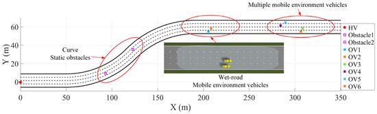
Figure 4.
Overall simulation environment.
Scene 1 consists of a straight 50 m section connected to two circular arc sections with a total length of 78.5 m, each having a curvature radius of 100 m, and no transition curves were set between each section of the road. The initial speed of the host vehicle (HV) is 0. In each of the second and third lanes, there is a static obstacle with a volume of 1 cubic meter. The vehicle trajectory is shown in Figure 5. In the initial stationary state of the HV, based on the lattice trajectory planning algorithm, it achieved safe passage around multiple obstacles on the continuous curved sections. By calculating the Euclidean distance between each trajectory point and the obstacles, the minimum distances between the vehicle trajectory and the two obstacles are 3.03 m and 2.97 m, respectively, meeting the vehicle safety envelope. By directly incorporating the curvature constraint as an optimization condition to limit the lateral acceleration and the vehicle’s optimal speed curve, a moderate increase in speed in long-radius curves and more uniform longitudinal and lateral control are achieved. The vehicle’s driving trajectory always remains between the road boundary and the lane lines, and the obstacle avoidance process is continuous, smooth, and without sudden changes. This verifies the effectiveness and feasibility of the proposed method in the mixed scenarios of curved roads and obstacles. The overall trajectory exhibits good trajectory continuity, dynamic feasibility, and obstacle safety margin, which can meet the requirements of safety and real-time performance in high-speed scenarios.
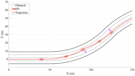
Figure 5.
Avoiding stationary obstacles on the curve.
In this study, an RLS observer was built on the Simulink simulation platform, and the longitudinal road adhesion coefficient estimation model was simulated and verified jointly with CarSim. The simulation results are shown in Figure 6. Between the driving distances of 200 to 260 m, the road adhesion coefficient suddenly changed from 0.85 to 0.3. Through the RLS algorithm, the estimated curve tracked the changes in the adhesion conditions, with good real-time performance. The average estimated error was 0.0124, and the estimation accuracy was relatively high.
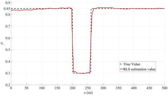
Figure 6.
Estimated results of road surface adhesion coefficient.
In Scene 2, there is a slippery road surface and moving obstacle vehicles in the first and second lanes. In Figure 7, based on the comprehensive framework for driving decision-making and trajectory planning constructed in this paper, the system can accurately identify sudden changes in road conditions. According to the simulation results in Section 3.1, when the HV reaches 200 m, the road adhesion coefficient suddenly changes from 0.85 to 0.3. At this point, the action instructions are issued by the decision-making layer, and the longitudinal and lateral coupling planning is smoothly converted to longitudinal speed planning. The HV slows down and maintains a safe distance from the preceding vehicle. After leaving the slippery road surface, the system switches back to the longitudinal and lateral coupling trajectory planning mode. Based on the environmental perception results, the decision module triggers the lane change and acceleration–overtaking actions and the HV accelerates and overtakes, effectively avoiding dynamic targets. Through the wet road–moving vehicle scenario, the intelligent decision-making and trajectory planning framework proposed in this paper has been verified to be able to coordinate multiple sources of information, reasonably switch planning modes, and effectively avoid high-risk situations such as skidding and rollover caused by insufficient adhesion under sudden road changes, thereby improving the environmental adaptability, safety, and stability of the autonomous driving system.
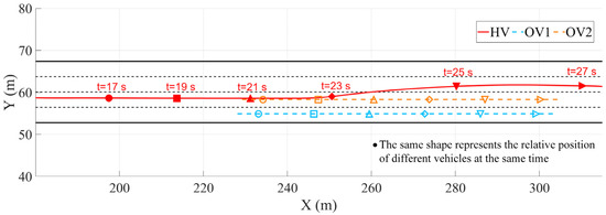
Figure 7.
Wet road.
Scene 3 is a complex scenario involving multiple moving vehicles. The HV is faced with multiple moving vehicles (ov3 to ov6) distributed continuously across different lanes, and needs to dynamically complete multiple lane changes and overtaking maneuvers. In Figure 8, the HV is traveling in the third lane. After detecting ov4 in the same lane ahead, the decision-making module actively plans the lane change strategy based on the surrounding traffic conditions and autonomously changes lanes to the second lane to complete the overtaking. During the continued driving process, the HV again recognizes ov3 in the current lane, and the system promptly completes the second right lane change, successfully returning to the third lane to complete the overtaking operation. Throughout the process, the trajectory planning module generates paths that maintain good continuity and feasibility, with smooth trajectory curves, timely obstacle avoidance behaviors, and no sudden changes or dangerous deviations. The system effectively integrates the results of multi-vehicle situation awareness and lateral dynamic constraints, achieving coordinated avoidance of multiple dynamic targets in dense traffic flows and demonstrating the advantages of the decision-making and planning framework proposed in this paper in terms of security.
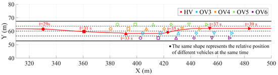
Figure 8.
Multiple-moving-vehicle environment.
To further verify the physical feasibility and security of the generated trajectories, the curves of longitudinal velocity, lateral acceleration, and front wheel angle changing with driving distance are extracted. These three parameters are extracted from the whole simulation process, including all three scenarios, as shown in Figure 9.
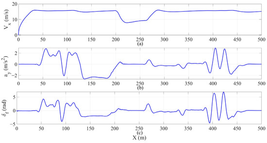
Figure 9.
(a) Longitudinal speed; (b) lateral acceleration; (c) front wheel angle.
In Figure 9a, the longitudinal velocity of the HV is shown. The initial speed is 0 m/s, and it accelerates smoothly to the desired speed of 16 m/s. During the obstacle avoidance process, there is a slight fluctuation. When it reaches 200 m, due to a sudden change in the road surface condition, the vehicle speed drops to 8 m/s. It maintains a safe distance and continues driving, then accelerates to overtake after leaving the slippery road surface. This verifies that the intelligent vehicle driving decisions and trajectory planning framework proposed in this paper fully considers the influence of road surface conditions, which is of great significance for improving driving safety.
The lateral acceleration curve of the HV is shown in Figure 9b. When HV is traveling in the curve in Scenario 1, the curvature radii of both sections of the curve are 100. Therefore, there are downward and upward centrifugal accelerations of 2.56 m/s2 in the lateral direction. On the first section of the curve, due to the lane change to the third lane to avoid obstacles, the lateral acceleration is pulled back. On the second section of the curve, there is no lane change behavior, and the lateral acceleration fluctuates slightly. In Scenario 3, multiple obstacle vehicles are interlaced in adjacent lanes, forming a dynamic dense traffic environment. The HV needs to perform multiple consecutive lane changes and obstacle avoidance actions. The lateral acceleration curve in this section shows high-frequency fluctuations, with the maximum value being ±2.8 m/s2. This mainly reflects the continuous lateral maneuvering behavior of the vehicle in complex traffic scenarios, but it has never exceeded the adhesion limit allowed range (), and there is a certain safety margin without exceeding the physical limit of vehicle stability.
In Figure 9c, there is a curve showing the variation of the front wheel angle. The vehicle maintains excellent steering control performance during the driving process. There are obvious fluctuations when encountering the high-density dynamic obstacle targets in Scenario 3, but the maximum angle amplitude is controlled within a range of ±7°, not exceeding the physical limitations of lateral control. The system responds quickly and acts reasonably during the lane changing–obstacle avoidance process, verifying the controllability and stability of the proposed planning framework in complex dynamic environments.
To verify the control method used in this paper, the lateral position and speed data were extracted from the planning results, and corresponding data were also obtained from the control results. The lateral position error and speed error were calculated. The parameter comparison and error results are shown in Figure 10, Figure 11 and Figure 12.
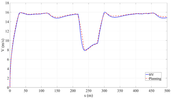
Figure 10.
Vehicle speed tracking.
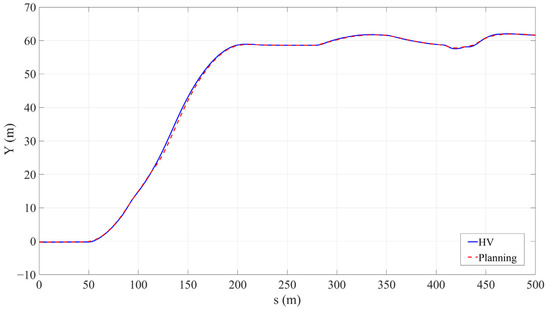
Figure 11.
Lateral position tracking.
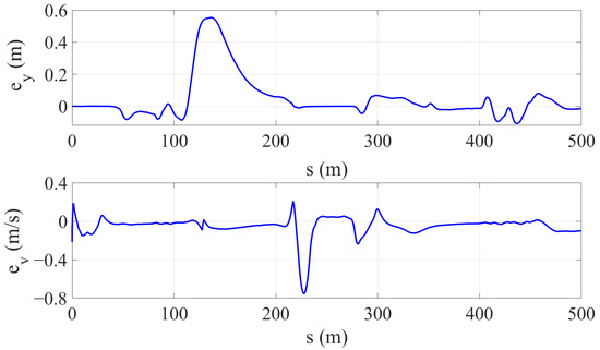
Figure 12.
Lateral position and velocity tracking error.
To present the accuracy of the control algorithm more intuitively, the root mean square errors of the lateral displacement and longitudinal velocity are calculated. The maximum errors of the lateral displacement and longitudinal velocity are shown in Table 3.
Table 3.
Quantitative index.
In this table, it can be seen that in Scenario 1, due to the main vehicle avoiding obstacles in consecutive curves, the peak value of the lateral position error is 0.516 m. However, through calculation, the root mean square error is 0.125 m per second, proving that the overall lateral position error is relatively small. In Scenario 2, there is a slippery road surface, and the main vehicle needs to slow down and follow closely during driving. The peak value of the speed tracking error is 0.781 m, and the root mean square error is 0.230 m per second, still at an excellent level. This confirms that the tracking method adopted in this paper has good tracking accuracy.
6. Summary and Future Work
This paper focuses on the key issues of vehicle decision-making and trajectory planning in intelligent driving systems, and proposes a vehicle driving decision-making and trajectory planning framework that comprehensively considers the influencing factors of vehicles and roads. Various scenarios were constructed for experimental verification. The main work included a lane-level driving decision-making mechanism based on environmental perception information, fully considering key factors such as surrounding vehicle information, lane boundaries, and road adhesion conditions. The lattice longitudinal–lateral coupling trajectory planning method was improved, generating fifth-order polynomial lateral trajectories based on the decision results and planning longitudinal speed based on a cubic acceleration model, ensuring consistency of longitudinal and lateral movements while meeting obstacle avoidance and stability requirements. The MPC algorithm and dual PID algorithm were used to achieve precise trajectory tracking and stable control of intelligent vehicles in different scenarios. Finally, a complex traffic scene including continuous obstacle avoidance in curves, slippery road surfaces, and multiple moving vehicles was constructed through the joint simulation platform to verify the comprehensive capabilities of the proposed method in dynamic decision-making, environmental adaptability, and safety control.
In future research, we will consider enhancing the dynamic traffic scenario adaptability of the autonomous driving system. By introducing multi-vehicle interaction game modeling mechanisms and other methods, we will strengthen the multi-agent coordination and conflict avoidance capabilities in complex traffic scenarios. At the same time, we will introduce driver style modeling methods to conduct personalized trajectory optimization for different driving behavior patterns such as aggressive and conservative types, thereby improving the human–vehicle collaboration experience and the explainability of driving behaviors. Finally, we will consider conducting hardware-in-the-loop verification and real road vehicle tests. We will build an HIL platform including ECU, IMU, GPS, and onboard Ethernet communication to test the performance and timeliness of the algorithm in a real-time closed loop and conduct road experiments under different adhesion coefficients (slippery, icy), multi-sensor error injection, and external disturbance scenarios to systematically evaluate the stability and safety margin of the method.
Author Contributions
Conceptualization, Y.Y.; methodology, Y.Y. and C.D.; software, C.D.; validation, Y.Y. and C.D.; formal analysis, C.D.; investigation, Y.W.; resources, Y.Y.; data curation, Y.Y. and C.D.; writing—original draft preparation, C.D.; writing—review and editing, C.D.; visualization, Y.W.; supervision, Y.W.; project administration, D.P.; funding acquisition D.P. All authors have read and agreed to the published version of the manuscript.
Funding
This research was funded by the Key Project of the National Key Laboratory of Advanced Off-Road Systems Fund (201NKL-2024-P-02-07) and National Natural Science Foundation of China (NSFC) under grant 52332013.
Data Availability Statement
The data reported in this manuscript are accessible upon reasonable request to the corresponding author.
Conflicts of Interest
The authors declare no conflicts of interest.
Abbreviations
The following abbreviations are used in this manuscript.
| RLS | recursive least squares |
| MPC | model predictive control |
| DP | dynamic programming |
| QP | quadratic programming |
| HV | host vehicle |
| OV | obstacle vehicle |
| PID | proportional–integral–differential |
References
- Zhu, B.; Jia, S.Z.; Zhao, J. A Review of Research on Decision-Making and Planning for Autonomous Vehicles. China J. Highw. Eng. 2024, 37, 215–240. [Google Scholar]
- Claussmann, L.; Revilloud, M.; Gruyer, D.; Glaser, S. A review of motion planning for highway autonomous driving. IEEE Trans. Intell. Transp. Syst. 2020, 21, 1826–1848. [Google Scholar] [CrossRef]
- Guerrieri, M.; Parla, G.; Corriere, F. A new methodology to estimate deformations of longitudinal safety barrier. ARPN J. Eng. Appl. Sci. 2013, 8, 763–769, ISSN 1819-6608. [Google Scholar]
- Li, B.; Yin, Z.; Ouyang, Y.; Zhang, Y.; Zhong, X.; Tang, S. Online trajectory replanning for sudden environmental changes during automated parking: A parallel stitching method. IEEE Trans. Intell. Veh. 2022, 7, 748–757. [Google Scholar] [CrossRef]
- Yagüe-Cuevas, D.; Paz-Sesmero, M.; Marín-Plaza, P.; Sanchis, A. Organizing Planning Knowledge for Automated Vehicles and Intelligent Transportation Systems. IET Intell. Transp. Syst. 2024, 18 (Suppl. S1), 2977–2994. [Google Scholar] [CrossRef]
- Li, X.X.; Ren, M.L. Road Adhesion Coefficient Estimation: Physics-Informed Deep Learning Method with Vehicle Dynamics Model. Expert Syst. Appl. 2025, 260, 0957–4174. [Google Scholar] [CrossRef]
- Zhou, G.; Gao, C.; Wang, Y. A Road Adhesion Coefficient Estimation Method Based on Feature Screening and Ensemble Learning. Proc. Inst. Mech. Eng. Part D J. Automob. Eng. 2025, 09544070251319071. [Google Scholar] [CrossRef]
- Zhao, T.; He, J.; Lv, J.; Min, D.; Wei, Y. A Comprehensive Implementation of Road Surface Classification for Vehicle Driving Assistance: Dataset, Models, and Deployment. IEEE Trans. Intell. Transp. Syst. 2023, 24, 8361–8370. [Google Scholar] [CrossRef]
- Guo, Y.; Guo, Z.; Wang, Y.; Yao, D.; Li, B.; Li, L. A Survey of Trajectory Planning Methods for Autonomous Driving—Part I: Unstructured Scenarios. IEEE Trans. Intell. Veh. 2024, 9, 5407–5434. [Google Scholar] [CrossRef]
- Han, Y.; Lu, Y.; Wang, H.; Wang, Y. A New Preprocessment Method for Road Peak Adhesion Coefficient Fusion Estimation. Proc. Inst. Mech. Eng. Part D J. Automob. Eng. 2024, 238, 224–240. [Google Scholar] [CrossRef]
- Xu, Z.; Lu, Y.; Chen, N.; Han, Y. Integrated Adhesion Coefficient Estimation of 3D Road Surfaces Based on Dimensionless Data-Driven Tire Model. Machines 2023, 11, 189. [Google Scholar] [CrossRef]
- Wang, Y. An Integrated Scheme for Coefficient Estimation of Tire–Road Friction with Mass Parameter Mismatch Under Complex Driving Scenarios. IEEE Trans. Ind. Electron. 2022, 69, 13337–13347. [Google Scholar] [CrossRef]
- Wang, Y.; Hu, J.; Wang, F. Tire Road Friction Coefficient Estimation: Review and Research Perspectives. Chin. J. Mech. Eng. 2022, 35, 6. [Google Scholar] [CrossRef]
- Wang, X.; Gu, L.; Dong, M.M.; Li, X.L. State estimation of tire-road friction and suspension system coupling dynamic in braking process and change detection of road adhesive ability. Proc. Inst. Mech. Eng. Part D J. Automob. Eng. 2022, 236, 1170–1187. [Google Scholar]
- Wang, Y.; Tian, F.; Wang, J. A Bayesian expectation maximization algorithm for state estimation of intelligent vehicles considering data loss and noise uncertainty. Sci. China Technol. Sci. 2025, 68, 1220801. [Google Scholar] [CrossRef]
- Wang, Y.; Yin, G.; Hang, P.; Zhao, J.; Lin, Y.; Huang, C. Fundamental Estimation for Tire Road Friction Coefficient: A Model-Based Learning Framework. IEEE Trans. Veh. Technol. 2025, 74, 481–493. [Google Scholar] [CrossRef]
- Liu, R.Q.; Wei, M.X.; Sang, N.; Wei, J.W. Research on Curved Path Tracking Control for Four-Wheel Steering Vehicle considering Road Adhesion Coefficient. Math. Probl. Eng. 2020, 18, 3108589. [Google Scholar] [CrossRef]
- Ping, X.; Cheng, S.; Yue, W.; Du, Y.; Wang, X.; Li, L. Adaptive Estimations of Tyre–Road Friction Coefficient and Body’S Sideslip Angle Based on Strong Tracking and Interactive Multiple Model Theories. Proc. Inst. Mech. Eng. Part D J. Automob. Eng. 2020, 234, 3224–3238. [Google Scholar] [CrossRef]
- Somalwar, R.S.; Kadwane, S.G.; Ruikar, J. Advanced Active Islanding Method with Recursive Least Square for Microgrid. IEEE J. Emerg. Sel. Top. Ind. Electron. 2024, 5, 1055–1064. [Google Scholar] [CrossRef]
- Wu, D.; Zhang, L.B.; Zhang, Y.X. Visual Detection Method of Vehicle Braking Time Series Based on Slip Rate Identification. J. Jilin Univ. (Eng. Ed.) 2021, 51, 206–216. [Google Scholar]
- Guo, C.; Wang, X.L.; Su, L.L.; Wang, Y.S. Safety Distance Model for Longitudinal Collision Avoidance of Logistics Vehicles Considering Slope and Road Adhesion Coefficient. Proc. Inst. Mech. Eng. Part D J. Automob. Eng. 2021, 235, 498–512. [Google Scholar] [CrossRef]
- He, R.; Feng, H.P. Road Surface Identification Algorithm Based on Peak Adhesion Coefficient Surface. J. Jilin Univ. (Eng. Ed.) 2020, 50, 1245–1256. [Google Scholar]
- Hussain, K.; Moreira, C.; Pereira, J.; Jardim, S.; Jorge, J. A Comprehensive Literature Review on Modular Approaches to Autonomous Driving: Deep Learning for Road and Racing Scenarios. Smart Cities 2025, 8, 79. [Google Scholar] [CrossRef]
- Zhang, Y.; Xu, Q.; Wang, J.; Wu, K.; Zheng, Z.; Lu, K. A Learning-Based Discretionary Lane-Change Decision-Making Model with Driving Style Awareness. IEEE Trans. Intell. Transp. Syst. 2023, 24, 68–78. [Google Scholar] [CrossRef]
- Yang, H.; Zhou, Y.; Wu, J.; Liu, H.; Yang, L.; Lv, C. Human-Guided Continual Learning for Personalized Decision-Making of Autonomous Driving. IEEE Trans. Intell. Transp. Syst. 2025, 26, 5435–5447. [Google Scholar] [CrossRef]
- Huang, J.; Wu, B.; Duan, Q.; Dong, L.; Yu, S. A Fast UAV Trajectory Planning Framework in RIS-Assisted Communication Systems with Accelerated Learning via Multithreading and Federating. IEEE Trans. Mob. Comput. 2025, 24, 6870–6885. [Google Scholar] [CrossRef]
- Xia, T.; Chen, H. A Survey of Autonomous Vehicle Behaviors: Trajectory Planning Algorithms, Sensed Collision Risks, and User Expectations. Sensors 2024, 24, 4808. [Google Scholar] [CrossRef]
- Zheng, Y.; Yi, L.; Wei, Z. A Survey of Dynamic Graph Neural Networks. Front. Comput. Sci. 2025, 19, 196323. [Google Scholar] [CrossRef]
- Gao, S.; Huang, S.; Xiang, C.; Lee, T.H. A Review of Optimal Motion Planning for Unmanned Vehicles. J. Mar. Sci. Technol. 2020, 28, 321–330. [Google Scholar]
- Receveur, J.; Victor, S.; Melchior, P. Autonomous Car Decision Making and Trajectory Tracking Based on Genetic Algorithms and Fractional Potential Fields. Intel. Serv. Robot. 2020, 13, 315–330. [Google Scholar] [CrossRef]
- Menon, A.S.; Damm, E.R.; Howard, T.M. Homotopy-Aware Efficiently Adaptive State Lattices for Mobile Robot Motion Planning in Cluttered Environments. IEEE Robot. Autom. Lett. 2025, 10, 947–954. [Google Scholar] [CrossRef]
- Morsali, M.; Frisk, E.; Åslund, J. Spatio-Temporal Planning in Multi-Vehicle Scenarios for Autonomous Vehicle Using Support Vector Machines. IEEE Trans. Intell. Veh. 2021, 6, 611–621. [Google Scholar] [CrossRef]
- Zhang, H.Y.; Du, L.L. Real-Time Executable Platoon Formation Approach Using Hierarchical Cooperative Motion Planning Framework. Transp. Res. Part C Emerg. Technol. 2025, 171, 104942. [Google Scholar] [CrossRef]
- ISO 3888-1:2018; Passenger Cars—Test Track for a Severe Lane-Change Manoeuvre—Part 1: Double Lane-Change. International Organization for Standardization: Geneva, Switzerland, 2018.
- Richter, M.; Kabza, H. Strategic dynamic traffic routing algorithm for globally optimized urban traffic. IEEE Intell. Veh. Symp. (IV) 2013, 756–762. [Google Scholar] [CrossRef]
- Wang, J.; Chu, L.; Zhang, Y.; Mao, Y.; Guo, C. Intelligent Vehicle Decision-Making and Trajectory Planning Method Based on Deep Reinforcement Learning in the Frenet Space. Sensors 2023, 23, 9819. [Google Scholar] [CrossRef] [PubMed]
- Wang, J.; Yan, Y.; Zhang, K.; Chen, Y.; Cao, M.; Yin, G. Path planning on large curvature roads using driver-vehicle-road system based on the kinematic vehicle model. IEEE Trans. Veh. Technol. 2022, 71, 311–325. [Google Scholar] [CrossRef]


Disclaimer/Publisher’s Note: The statements, opinions and data contained in all publications are solely those of the individual author(s) and contributor(s) and not of MDPI and/or the editor(s). MDPI and/or the editor(s) disclaim responsibility for any injury to people or property resulting from any ideas, methods, instructions or products referred to in the content. |
© 2025 by the authors. Licensee MDPI, Basel, Switzerland. This article is an open access article distributed under the terms and conditions of the Creative Commons Attribution (CC BY) license (https://creativecommons.org/licenses/by/4.0/).