
Parameters Identification for a Composite Piezoelectric Actuator Dynamics


Abstract
:1. Introduction
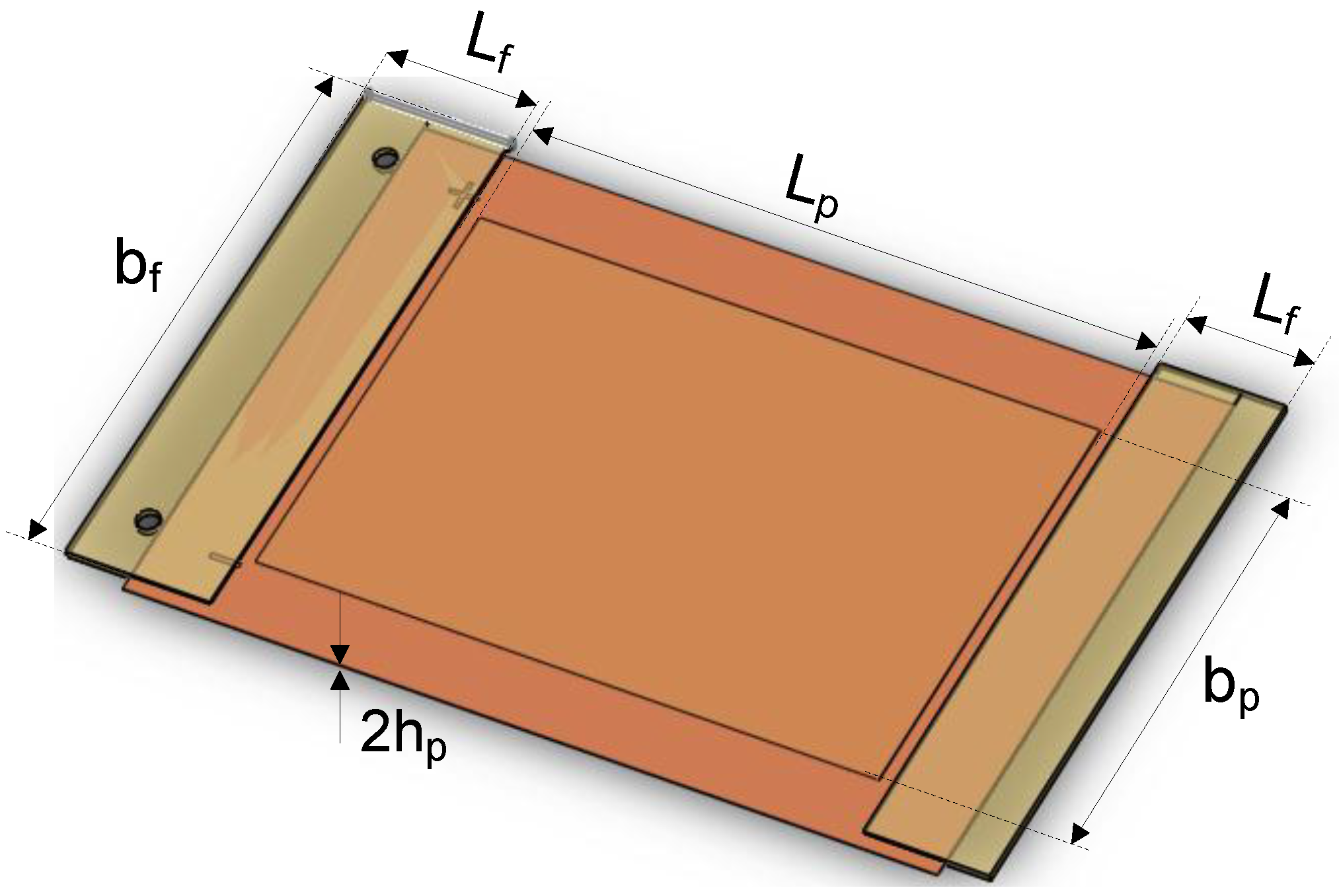
2. Prototype of the PZT Bimorph Actuator


| Variable | Fiberglass | MFC |
|---|---|---|
| Length (mm) | Lf = 17 | Lp = 85 (active length) |
| Width (mm) | bf = 75 | bp = 56 |
| Height (mm) | hf = 0.5 | hp = 0.3 |
| PZT strain constant d33 (m/V) | N/A | d33 = 4.275 × 10⁻¹⁰ |
| Electrode spacing es (mm) | N/A | es = 0.5 |
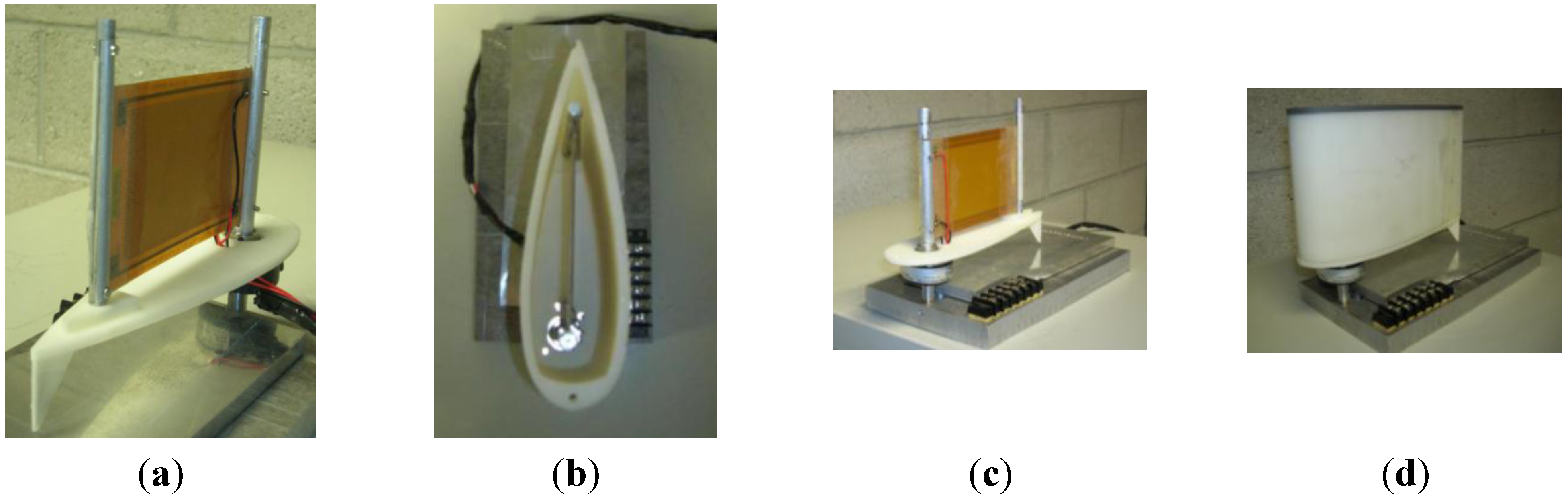
3. PZT Bimorph-Actuated Smart Fin

4. Modeling

Identification of the Damping, Hysteresis and Backlash Parameters

| Parameter | Value |
|---|---|
| Encoding technique | Binary |
| Number of bits | 3 for discrete, 14 for continuous |
| Population | 400 |
| Elitism | 50% |
| Crossover technique | 2-points |
| Mutation rate | 0.01 |
| Generation | 1000 |
| Parameter | Parameter Range | |||
|---|---|---|---|---|
| Lower Limit | Upper Limit | Gain | ||
| Damping | μ | 0 | 1 | 1 |
| δ | 0 | 300 | 300 | |
| Hysteresis | α | −0.1 | 0 | −0.1 |
| β | −0.1 | 0 | −0.1 | |
| γ | −0.1 | 0 | −0.1 | |
| Backlash | a1 | 0 | 2 | 2 |
| a2 | 0 | 2 | 2 | |
| Parameter | Number of Nodes | Lower Limit | Upper Limit | Binary Coding | Resolution |
|---|---|---|---|---|---|
| Input nodes | 2 | N/A | N/A | N/A | N/A |
| Output nodes | 7 | N/A | N/A | N/A | N/A |
| Hidden nodes | Adaptive | 2 | 9 | 3 bits | 1 |
| Learning rules | Adaptive | 1 | 8 | 3 bits | 1 |
| Connection weights | NA | −10 | 10 | 14 bits | 1.2 × 10⁻³ |
| Frequency | 0.25 Hz | 0.5 Hz | 1.0 Hz | |
|---|---|---|---|---|
| Voltage | ||||
| 375 V | Case 1 | Case 2 | Case 3 | |
| 500 V | Case 4 | Case 5 | Case 6 | |
| 750 V | Case 7 | Case 8 | Case 9 | |
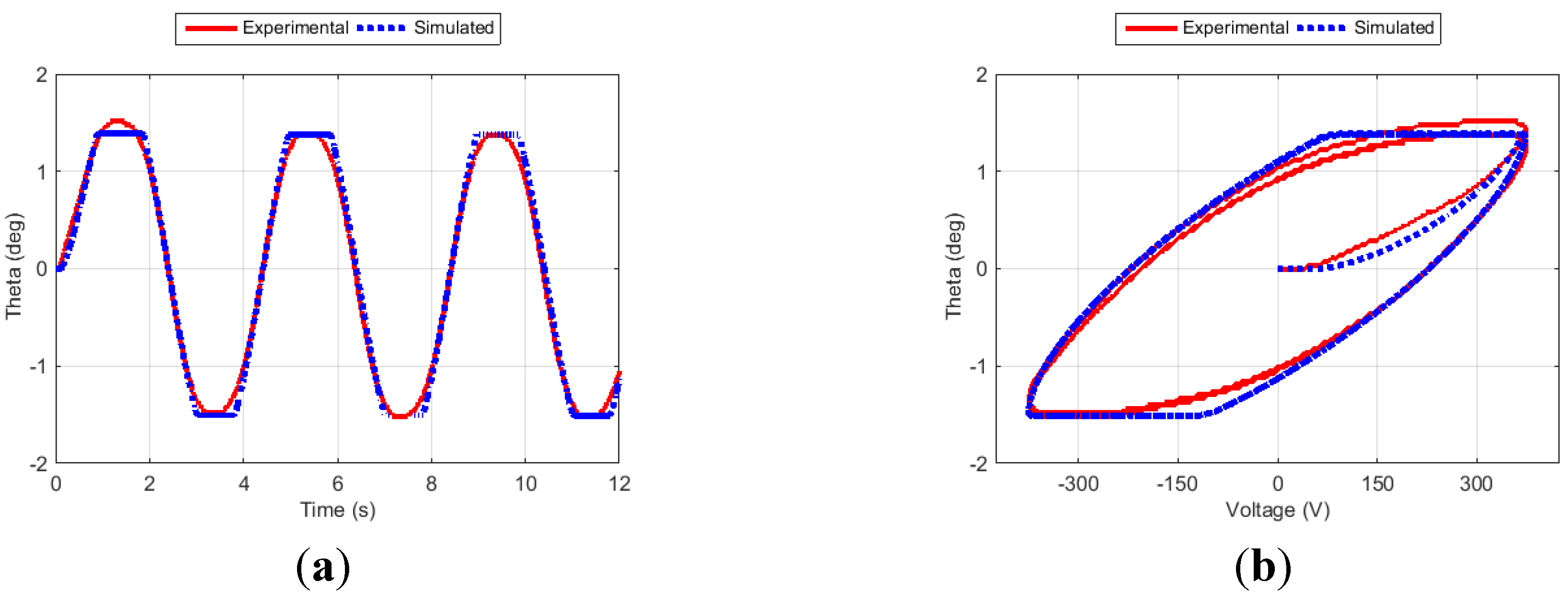
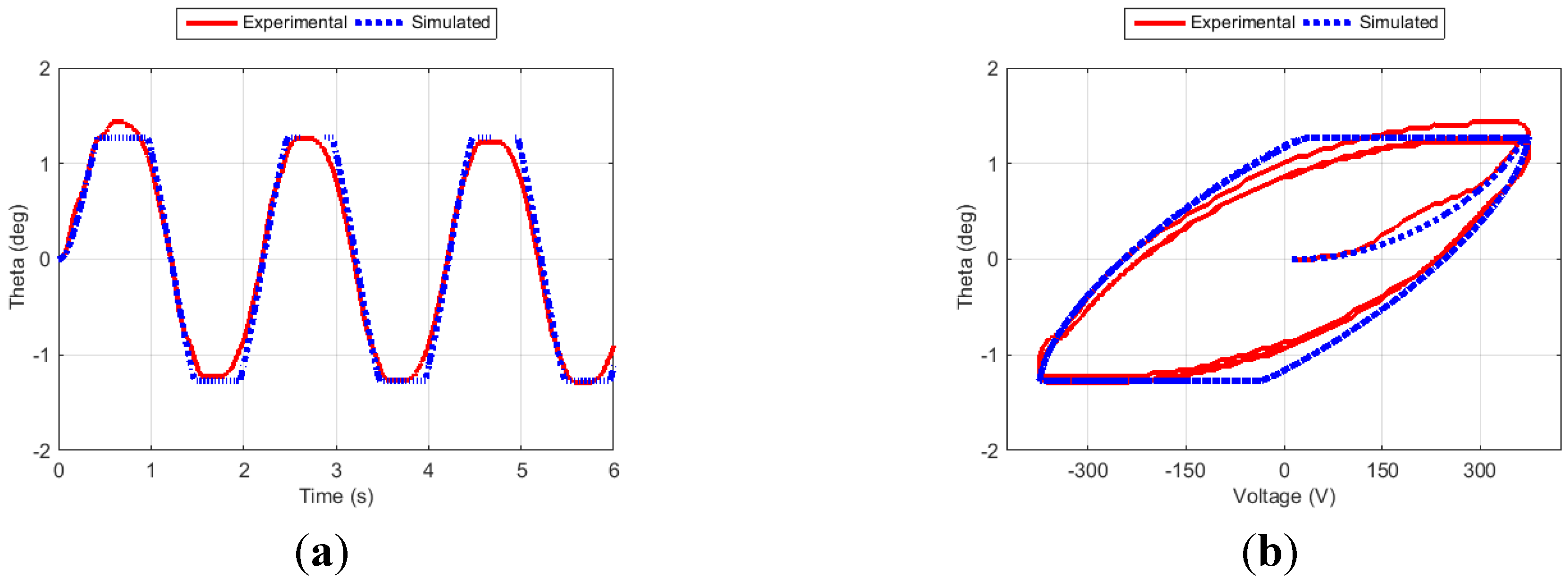
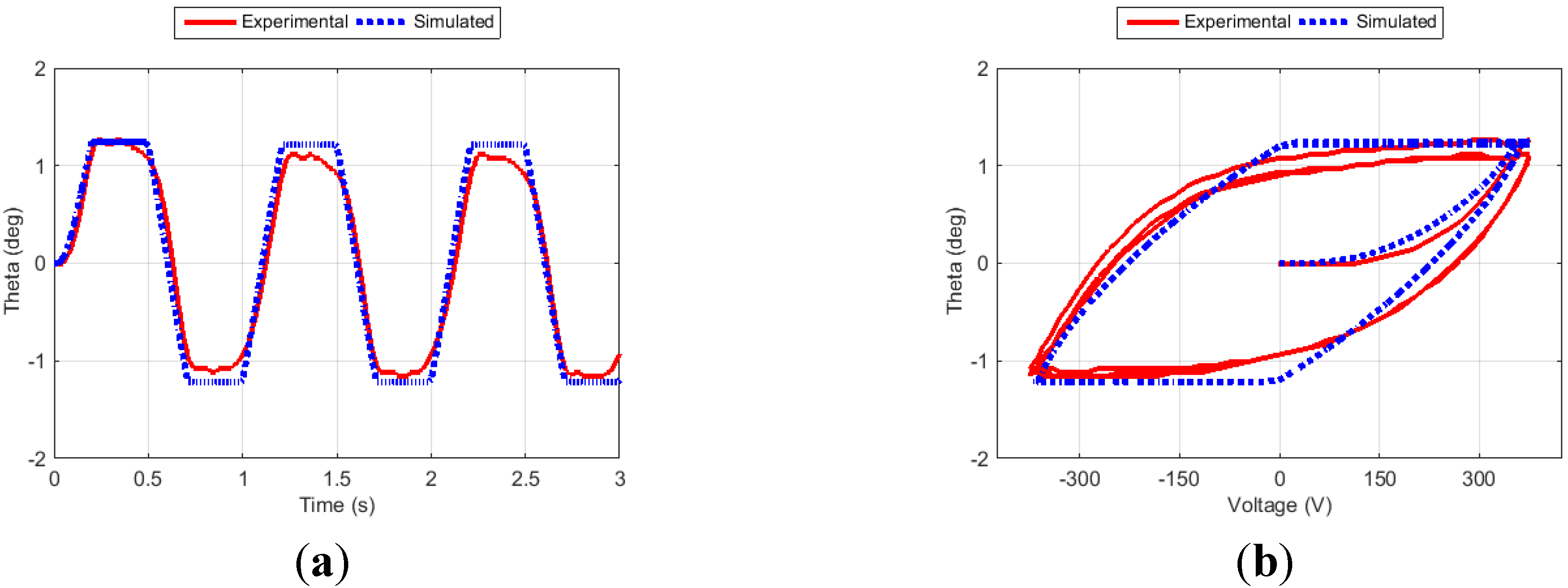
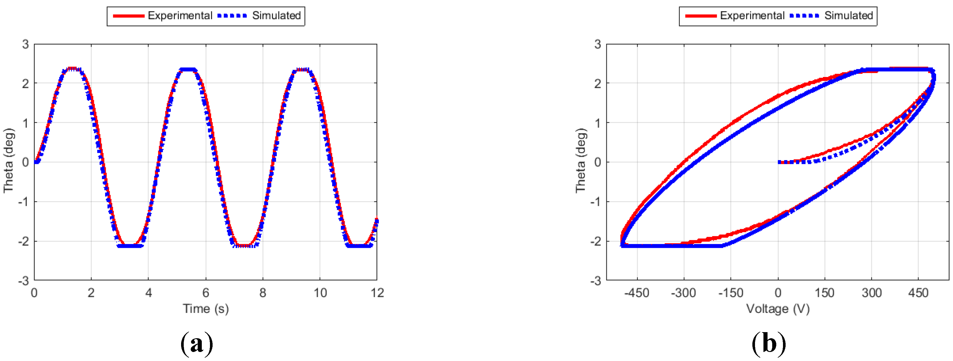
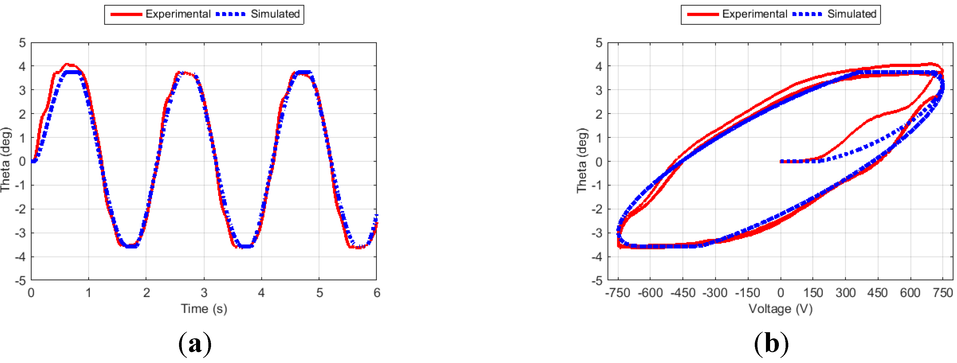
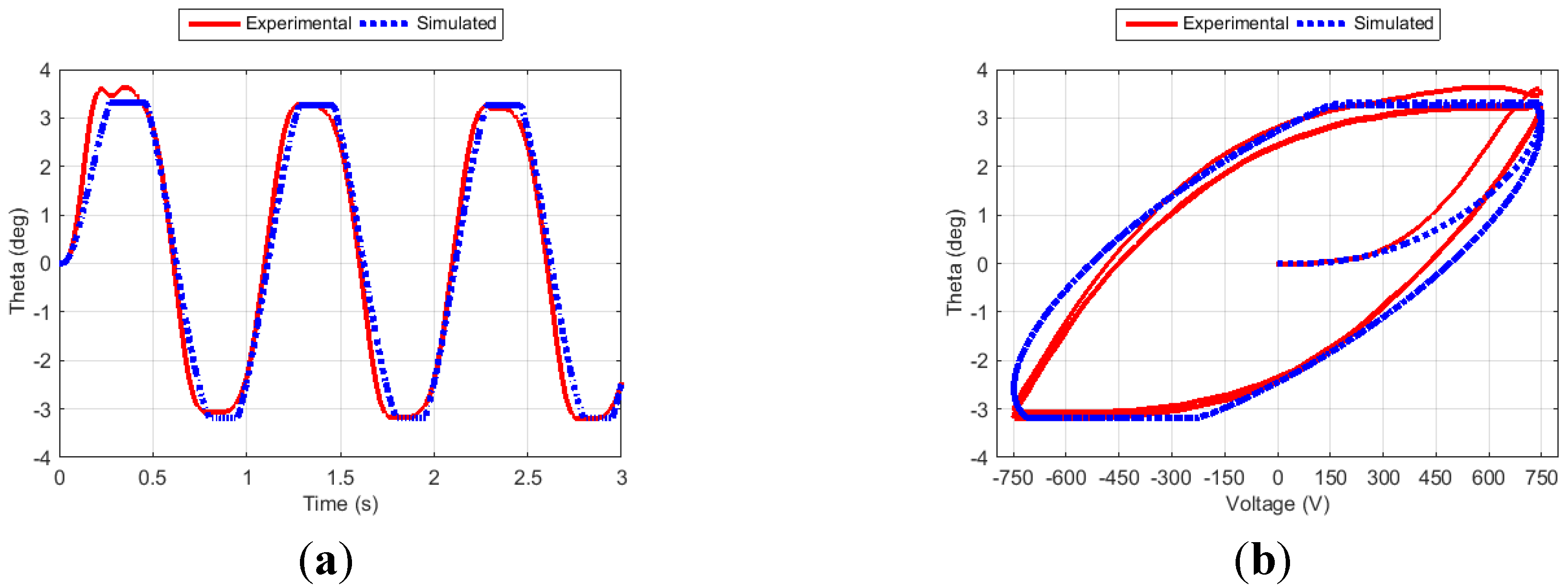
5. Results

| Case 1 | Case 5 | Case 6 | Case 7 | ||
|---|---|---|---|---|---|
| Damping | δ | 0.312 | 0.093 | 0 | 0.128 |
| μ | 98.650 | 94.666 | 75.626 | 109.210 | |
| Hysteresis | α | 0 | 0 | 0 | 0 |
| β | −7.49 × 10⁻² | −7.88 × 10⁻² | −8.06 × 10⁻² | −8.23 × 10⁻² | |
| γ | −6.51 × 10⁻² | −7.20 × 10⁻² | −7.84 × 10⁻² | −5.30 × 10⁻² | |
| Backlash | a1 | 0 | 0 | 0 | 0.281 |
| a2 | 0 | 0 | 0 | 0.294 |


6. Model Validation
| Case 2 | Case 3 | Case 4 | Case 8 | Case 9 | ||
|---|---|---|---|---|---|---|
| Damping | δ | 0.124 | 0 | 0.219 | 0.029 | 0 |
| μ | 93.534 | 72.812 | 104.47 | 97.144 | 81.792 | |
| Hysteresis | α | 0 | 0 | 0 | 0 | 0 |
| β | −7.61 × 10⁻² | −7.92 × 10⁻² | −7.75 × 10⁻² | −8.34 × 10⁻² | −8.32 × 10⁻² | |
| γ | −8.00 × 10⁻² | −8.44 × 10⁻² | −6.55 × 10⁻² | −5.59 × 10⁻² | −6.57 × 10⁻² | |
| Backlash | a1 | 0 | 0 | 0.041 | 0.149 | 0 |
| a2 | 0 | 0 | 0 | 0.344 | 0.255 |
| Excitation Frequency (Hz) | |||
|---|---|---|---|
| Amplitude↓ | 0.25 | 0.50 | 1.00 |
| 375 V | 1.42 | 2.08 | 2.38 |
| 500 V | 2.49 | 1.96 | 1.51 |
| 750 V | 5.64 | 3.23 | 6.78 |


| Excitation Frequency (Hz) | |||
|---|---|---|---|
| Amplitude↓ | 0.25 | 0.50 | 1.00 |
| 375 V | 0.312 | 0.124 | 0 |
| 500 V | 0.219 | 0.093 | 0 |
| 750 V | 0.128 | 0.029 | 0 |
| Excitation Frequency (Hz) | |||
|---|---|---|---|
| Amplitude↓ | 0.25 | 0.50 | 1.00 |
| 375 V | 98.650 | 93.534 | 72.812 |
| 500 V | 104.47 | 94.666 | 75.626 |
| 750 V | 109.210 | 97.144 | 81.792 |
| V (volts) | f (Hz) | Yintercept | Coefficient of Determination R2 |
|---|---|---|---|
| 0.0020 p = 0.001 | −36.525 p < 0.001 | 102.361 p < 0.001 | 0.988 |
| Excitation Frequency (Hz) | |||
|---|---|---|---|
| Amplitude↓ | 0.25 | 0.50 | 1.00 |
| 375 V | 0 | 0 | 0 |
| 500 V | 0.041 | 0 | 0 |
| 750 V | 0.281 | 0.149 | 0 |
| Excitation Frequency (Hz) | |||
|---|---|---|---|
| Amplitude↓ | 0.25 | 0.50 | 1.00 |
| 375 V | 0 | 0 | 0 |
| 500 V | 0 | 0 | 0 |
| 750 V | 0.294 | 0.344 | 0.255 |
7. Conclusions
Acknowledgments
Author Contributions
Conflicts of Interest
Appendix
Appendix A: Backlash Operators
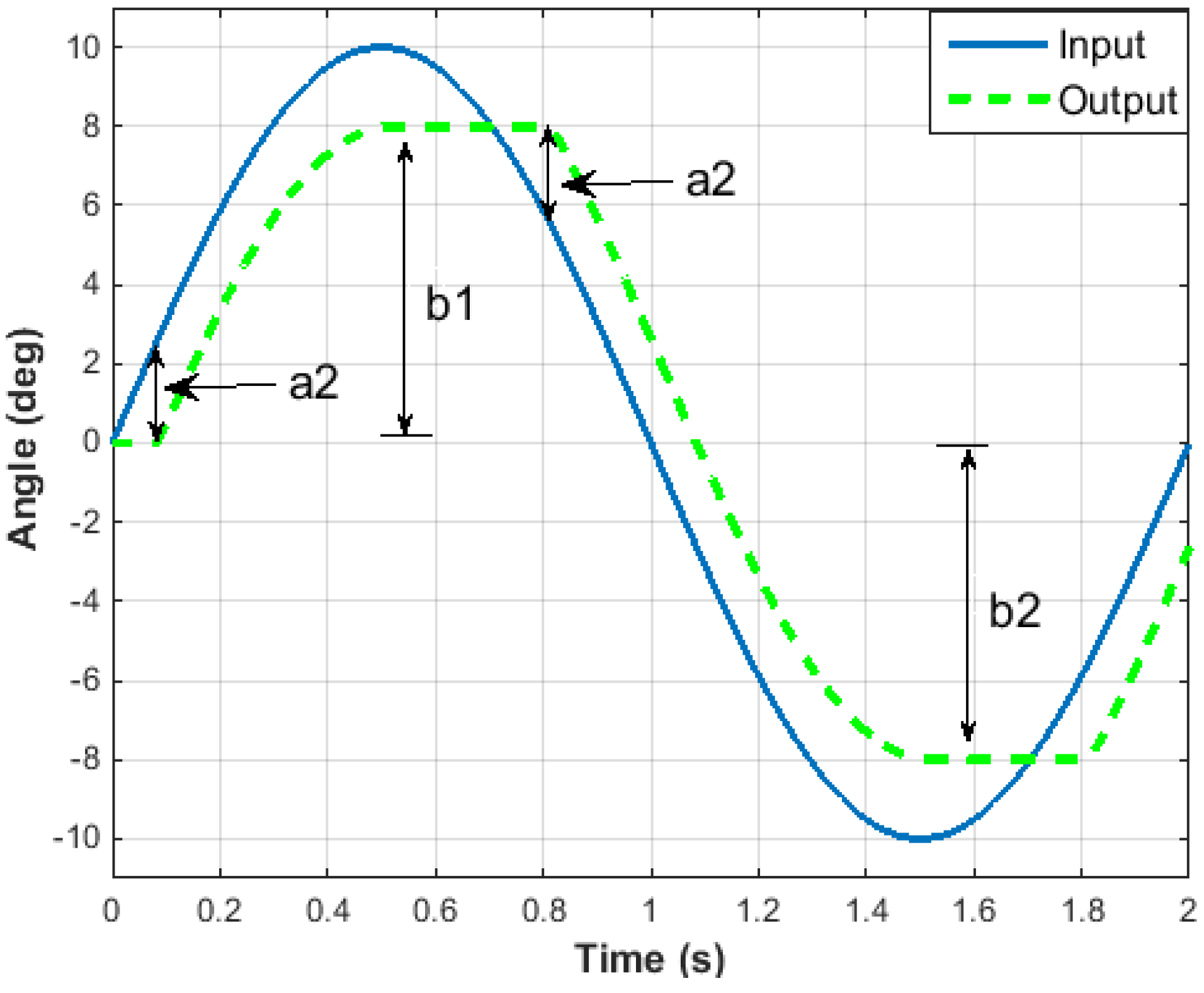
Appendix B: Identification of the Saturation Parameters
| Excitation Frequency (Hz) | |||
|---|---|---|---|
| Amplitude↓ | 0.25 | 0.50 | 1.00 |
| 375 V | b1 = 1.37 b2 = −1.50 | b1 = 1.26 b2 = −1.26 | b1 = 1.16 b2 = −1.16 |
| 500 V | b1 = 2.34 b2 = −2.12 | b1 = 2.05 b2 = −1.91 | b1 = 1.73 b2 = −1.66 |
| 750 V | b1 = 4.21 b2 = −4.03 | b1 = 3.74 b2 = −3.56 | b1 = 3.24 b2 = −3.17 |
| Parameter | V (volts) | f (Hz) | Yintercept | Coefficient of Determination R2 |
|---|---|---|---|---|
| b1 | 0.00645 p < 0.001 | −0.84771 p = 0.007 | −0.63061 p = 0.070 | 0.985 |
| b2 | −0.00622 p = 0.007 | 0.68371 p = 0.002 | 0.71011 p = 0.061 | 0.981 |
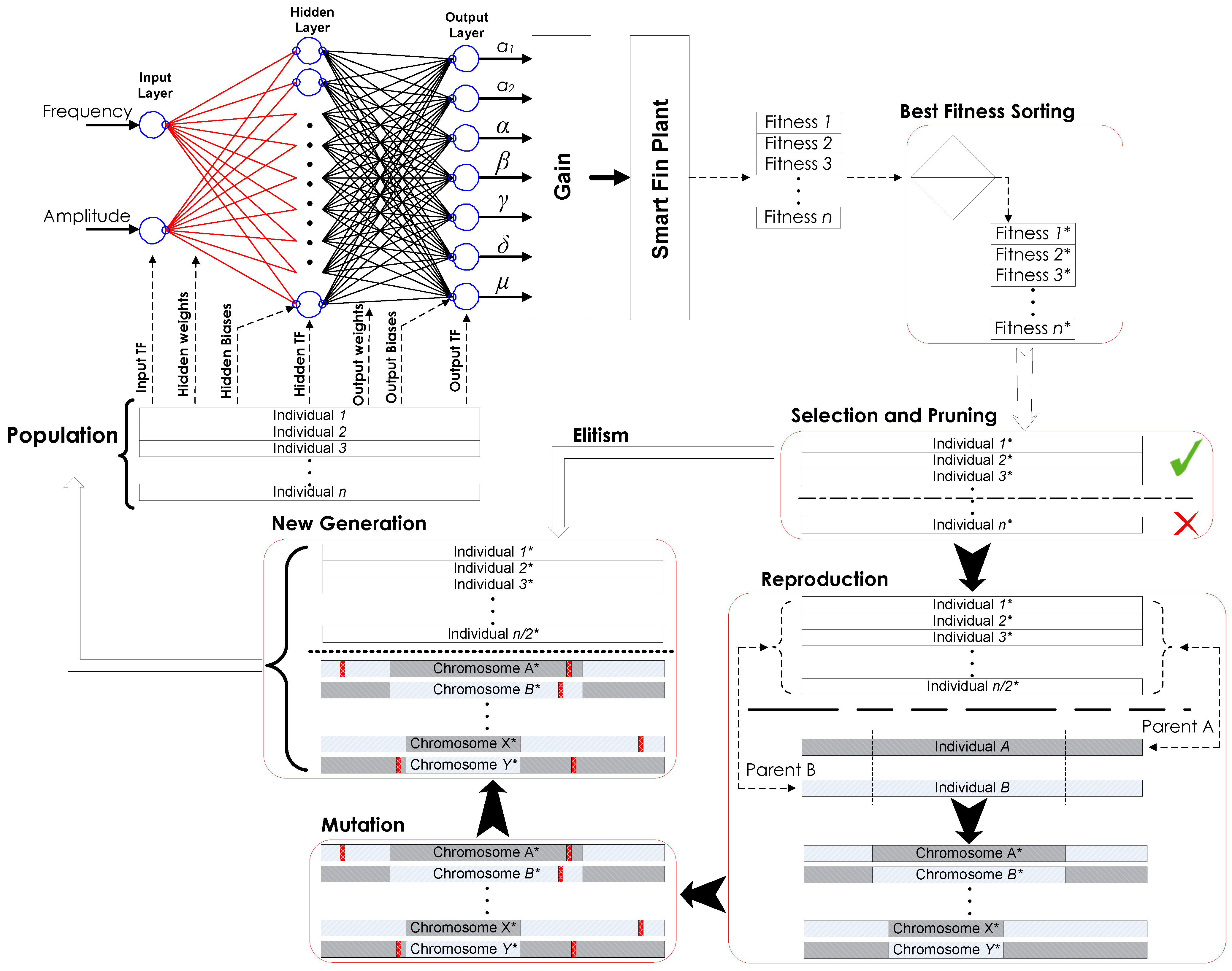
Appendix C: Hybrid Genetic Algorithm Neural Network
- Generate a random initial population where the NN characteristics are coded into the genetic material of each individual.
- Expand the compacted information of each individual and decode the genetic material into neural material, including; connection weights, biases, architecture and learning rules.
- Feed the four training cases for each individual at the input layer to identify the parameters of damping, hysteresis and backlash.
- Feed the parameters obtained at Step (3) into the dynamic model of the actuator to generate the simulated output angle.
- Evaluate the fitness of each individual. The individuals are then rearranged according to their fitness.
- Prune the least fitted individuals and select the best fitted ones as members of the new generation, as well as parents who will undergo the reproduction phases of crossover and mutation to produce new offspring for the next generation.
- Combine the new offspring with the best fitted individuals of the current generation to establish the population of the new generation.
- Repeat Steps 2 through 7 to progressively optimize a cost function until either the maximum number of generations is reached or there is no significant improvement recorded within the previous 200 successive generations.
Appendix D: NN Architecture
References
- Wilkie, W.; Bryant, R.; High, J.; Fox, R.; Hellbaum, R.; Jalink, A.; Little, B.; Mirick, P. Low-cost Piezocomposite Actuator for Structural Control Applications. Proc. SPIE 2000. [Google Scholar] [CrossRef]
- De Breuker, R.; Tiso, P.; Vos, R.; Barrett, R. Nonlinear Semi-Analytical Modeling of Post-Buckled Precompressed (PBP) Piezoelectric Actuators for UAV Flight Control. In Proceedings of the 47th AIAA/ASME/ASCE/AHS/ASC Structures, Structural Dynamics, and Materials Conference, Newport, RI, USA, 1–4 May 2006; pp. 1–13.
- LaCroix, B.; Ifju, P. Finite element modeling of macro fiber composite piezoelectric actuators on micro air vehicles. In Proceedings of the 53rd AIAA/ASME/ASCE/AHS/ASC Structures, Structural Dynamics, and Materials Conference, Honolulu, HI, USA, 23–26 April 2012; pp. 1–9.
- Barrett, R. Active Plate and missile wing development using directionally attached piezoelectric elements. AIAA J. 1994, 32, 601–609. [Google Scholar] [CrossRef]
- Barrett, R. All-moving active aerodynamic surface research. Smart Mater. Struct. 1995, 4, 65–74. [Google Scholar]
- Barrett, R.; Gross, R.; Brozoski, F. Missile flight control using active flexspar actuators. Smart Mater. Struct. 1996, 5, 121–128. [Google Scholar] [CrossRef]
- DeGiorgi, V.; Qidwal, A. An analysis of composite piezoelectric actuators incorporating nonlinear material behavior. In Proceedings of the ASME 2010 Conference on Smart Materials, Adaptive Structures and Intelligent Systems SMASIS 2010, Philadelphia, PA, USA, 28 September–1 October 2010; pp. 9–20.
- Trabia, M.; Yim, W.; Weinacht, P.; Mudupu, V. Control of a Projectile Smart Fin using an Inverse Dynamics-based Fuzzy Logic Controller. In Proceedings of the 21st Biennial Conference on Mechanical Vibration and Noise, Las Vegas, NV, USA, 4–7 September 2007; pp. 1823–1833.
- Mudupu, V.; Trabia, M.; Yim, W.; Weinacht, P. Design and validation of a fuzzy logic controller for a smart projectile fin with a piezoelectric macro-fiber composite bimorph actuator. Smart Mater. Struct. 2008, 17. [Google Scholar] [CrossRef]
- Trabia, M.; Yim, W.; Saadeh, M. Modeling of hysteresis and backlash for a smart fin with a piezoelectric actuator. J. Intell. Mater. Syst. Struct. 2011, 22, 1161–1176. [Google Scholar] [CrossRef]
- Aguirrea, G.; Janssens, T.; Brussel, H.V.; Al-Bender, F. Asymmetric-hysteresis compensation in piezoelectric actuators. Mech. Syst. Signal Process. 2012, 30, 218–231. [Google Scholar] [CrossRef]
- Li, P.; Yan, F.; Ge, C.; Wang, X.; Xu, L.; Guo, J.; Li, P. A simple fuzzy system for modelling of both rate-independent and rate-dependent hysteresis in piezoelectric actuators. Mech. Syst. Signal Process. 2013, 36, 182–192. [Google Scholar] [CrossRef]
- Novakova, K.; Mokry, P. Numerical simulation of mechanical behavior of a macro fiber composite piezoelectric actuator shunted by a negative capacitor. In Proceedings of the 10th International Workshop on Electronics, Control, Measurement and Signals (ECMS), Liberec, Czech Republic, 1–3 June 2011; pp. 1–5.
- Zhang, C.; Qiu, J.; Chen, Y.; Ji, H. Modeling hysteresis and creep behavior of macrofiber composite-based piezoelectric bimorph actuator. J. Intell. Mater. Syst. Struct. 2012, 24, 369–377. [Google Scholar] [CrossRef]
- Buchacz, A.; Placzek, M. The analysis of a composite beam with piezoelectric actuator based on the approximate method. J. Vibroeng. 2012, 14, 111–116. [Google Scholar]
- Novakova, K. Control of Static and Dynamic Mechanical Response of Piezoelectric Composite Shells: Applications to Acoustics and Adaptive Optics. Ph.D. Thesis, Technical University of Liberec, Liberec, Czech Republic, 2013. [Google Scholar]
- Piotr, K. Optimization and modeling composite structures with PZT layers. Adv. Mat. Res. 2014, 849, 108–114. [Google Scholar]
- Schaffer, J.; Whitley, D.; Eshelman, L. Combinations of Genetic Algorithms and Neural Networks: A Survey of the State of the Art. In Proceedings of the International Workshop on Combination of Genetic Algorithms and Neural Networks, Baltimore, MD, USA, 6 June 1992; pp. 1–37.
- Hinton, G.; Nowlan, S. How learning can guide evolution. Complex Syst. 1987, 1, 495–502. [Google Scholar]
- Ku, K.; Mak, M. Exploring the Effects of Lamarckian and Baldwinian Learning in Evolving Recurrent Neural Networks. In Proceedings of the IEEE International Evolutionary Computation, Indianapolis, IN, USA, 13–16 April 1997; pp. 617–621.
- Montana, D.; Davis, L. Training Feedforward Neural Networks using Genetic Algorithms. In Proceedings of the 11th International Joint Conference on Artificial Intelligence 1, Detroit, MI, USA, 20–26 August 1989; pp. 762–767.
- Zhang, B.; Mühlenbein, H. Evolving optimal neural networks using genetic algorithms with Occam’s razor. Complex Syst. 1993, 7, 199–220. [Google Scholar]
- Yao, X. Evolving artificial neural networks. Proc. IEEE 1999, 87, 1423–1447. [Google Scholar] [CrossRef]
- Fiszelew, A.; Britos, P.; Ochoa, A.; Merlino, H.; Fernández, E.; García-Martínez, R. Finding optimal neural network architecture using genetic algorithms. Res. Comput. Sci. 2007, 27, 15–24. [Google Scholar]
- Castillo, P.; Arenas, M.; Castellano, J.; Merelo, J.; Prieto, A.; Rivas, V.; Romero, G. Lamarckian evolution and the baldwin effect in evolutionary neural networks. Eprint arXiv:cs/0603004 2006. [Google Scholar]
- Kim, M.; Aggarwal, V.; O’Reilly, U.; Médrad, M.; Kim, W. Genetic Representations for Evolutionary Minimization of Network Coding Resources. In Proceedings of EvoWorkshops 2007, Valencia, Spain, 11–13 April 2007; pp. 21–31.
- Marwala, T. Control of complex systems using bayesian networks and genetic algorithm. IJES 2004, 5, 28–37. [Google Scholar]
- Su, C.; Yang, S.; Huang, W. A two-stage algorithm integrating genetic algorithm and modified Newton method for neural network training in engineering systems. Expert Syst. Appl. 2011, 38, 12189–12194. [Google Scholar] [CrossRef]
- Trabia, M.; Saadeh, M. A Hybrid Master-Slave Genetic Algorithm-Neural Network Approach for Modeling a Piezoelectric Actuator. In Proceedings of the Smart Materials, Adaptive Structures and Intelligent Systems, Stone Mountain, GA, USA, 19–21 September 2012; pp. 281–294.
- Istook, E.; Martinez, T. Improved backpropagation learning in neural networks with momentum. Int. J. Neural Syst. 2002, 12, 303–318. [Google Scholar] [CrossRef] [PubMed]
- Gori, M.; Tesi, A. On the problem of local minima in backpropagation. IEEE Trans. Pattern Anal. Mach. Intell. 1992, 14, 76–86. [Google Scholar] [CrossRef]
- Mangasarian, O.; Solodov, M. Backpropagation convergence via deterministic nonmonotone perturbed minimization. Optim. Methods Softw. 1994, 4, 103–116. [Google Scholar] [CrossRef]
- Lawrence, S.; Giles, L.; Tsoi, A. What Size Neural Network Gives Optimal Generalization? Convergence Properties of Backpropagation; Technical Report UMIACSTR-96-22; Institute for Advanced Computer Studies, University of Maryland: College Park, MD, USA, April 1996. [Google Scholar]
- Koehn, P. Combining genetic algorithms and neural networks: The encoding problem. Master’s Thesis, The University of Tennessee, Knoxville, TN, USA, 1994. [Google Scholar]
- Porto, V.; Fogel, D.; Fogel, L. Alternative neural network training methods. IEEE Expert 1995, 10, 16–22. [Google Scholar] [CrossRef]
- Gupta, J.; Sexston, R. Comparing backpropagation with a genetic algorithm for neural network training. Omega 1999, 27, 679–684. [Google Scholar] [CrossRef]
- Smart Material Macro Fiber Composite MFC. Available online: http://www.smart-material.com/media/Datasheet/MFC-V2.0-2011-web.pdf (accessed on 8 January 2015).
- Baburaj, V.; Okazaki, H.; Koga, T. Simulations on Dynamic Response of Adaptive SMA Composite Laminated Plates. In Proceedings of the 7th International Conference on Adaptive Structures, Rome, Italy, 23–25 September 1996; pp. 308–320.
- Wen, K. Equivalent linearization for hysteretic systems under random excitation. J. App. Mech. 1980, 47, 150–154. [Google Scholar] [CrossRef]
- Garmón, F.; Ang, W.; Khosla, P.; Riviere, C. Rate-dependent Inverse Hysteresis Feedforward Controller for Microsurgical Tool. In Proceedings of the 25th Annual Conference IEEE Engineering in Medicine and Biology Society, Cancun, Mexico, 17–21 September 2003; pp. 3415–3418.
- Beale, M.; Hagon, A.; Demuth, H. Neural Network Toolbox™ User’s Guide R2014b; The MathWorks, Inc.: Natick, MA, USA, 2014. Available online: https://www.mathworks.com/help/pdf_doc/nnet/nnet_ug.pdf (accessed on 5 January 2015).
© 2015 by the authors; licensee MDPI, Basel, Switzerland. This article is an open access article distributed under the terms and conditions of the Creative Commons Attribution license (http://creativecommons.org/licenses/by/4.0/).
Share and Cite
Saadeh, M.; Trabia, M. Parameters Identification for a Composite Piezoelectric Actuator Dynamics. Actuators 2015, 4, 39-59. https://doi.org/10.3390/act4010039
Saadeh M, Trabia M. Parameters Identification for a Composite Piezoelectric Actuator Dynamics. Actuators. 2015; 4(1):39-59. https://doi.org/10.3390/act4010039
Chicago/Turabian StyleSaadeh, Mohammad, and Mohamed Trabia. 2015. "Parameters Identification for a Composite Piezoelectric Actuator Dynamics" Actuators 4, no. 1: 39-59. https://doi.org/10.3390/act4010039