Abstract
Feed-forward control of hysteretic systems is a challenging task due to the hysteresis nonlinearity. Hysteresis models are utilized not only for identification, but also for hysteresis control. The feed-forward control, which is not an error-based (feedback-based) algorithm, plays a significant role in hysteresis control problems. Instead, it works based on knowledge about the process in the form of a mathematical model of the process. In feed-forward control problems, it is important to identify the inverse relationship of the output and input of the system, i.e., determining the mapping of the output and input of the system plays a key role in feed-forward controlling. This paper presents a new feed-forward controller model to control an actuator in a laboratory to tackle the restrictions of feedback control systems. For this purpose, first, a numerical model of a Proportional-Integral-Derivative (PID)-controlled actuator was created, and sets of numerical data of inputs and outputs of the plant were generated. Then, a least-squares support-vector machine (LS-SVM) hysteresis model was trained inversely on the generated data sets of the numerical modeling. Afterwards, to examine the efficacy of the proposed method for real-world hydraulic actuators in the presence of experimental errors and noise, sets of experimental data were obtained from physical modeling at KNTU’s Structural and Earthquake Engineering Laboratory (KSEEL). The results indicate the high performance of the proposed model.
1. Introduction
Hydraulic servo valve systems (HSS), which produce high torque and large forces with high speeds, are the critical components of the industrial field. The applications of HSS include, but are not limited to, manipulators, material test machines, fatigue testing, robotics, and aircraft [1]. In comparison to the other devices playing roles in the HSS, the role of the hydraulic servo valve systems is more advantageous. This is because of its high power and its high-speed response [1]. The response of hydraulic servo valve systems is highly nonlinear due to the directional changes of valve opening and friction; it would not be effortless to control such nonlinear systems using linear controllers [2,3]. One of the main goals in hydraulic control system problems is seeking a desired, satisfactory response of the system. An HSS consists of a motor, servo valve, controller, actuating cylinders, and measurement sensors. There are three main control categories in electrohydraulic problems: Position control, velocity control, and force control problems. In force control problems, the main goal is minimizing the force overshoot and preserving the load from failure. Bonchis et al. [4] introduced a new type of controller using acceleration feedback control, utilizing a variable-structure controller in the presence of friction nonlinearities. Sirouspour and Salcudean [5] proposed a nonlinear position controller for HSS, considering the valve dynamics presented in Lyapunov’s stability theories. The most commonly used controller in industrial applications is the Proportional-Integral-derivative (PID) controller [6,7], which uses the feedback of the systems to calculate the command of the system at each time step. In an HSS, the PID controller’s purpose is to minimize the difference between the desired set point and the measured output feedback of the plant by adjusting the command value sent to the valves [1,8]. It is well known that PID controllers show poor control performances for integrating processes and processes with large time delays. Moreover, they cannot incorporate ramp-type set-point changes or slow disturbances [9]. In feedback systems, small errors can propagate during the simulation. This error accumulation can significantly affect the simulation results, yielding inaccurate outcomes [10]. Many studies have been carried out on the design and tuning of PID controllers since 1942, in which Ziegler and Nichols presented their approaches. In addition, the specifications, stability, design, applications, and performance of PID controllers have been widely studied since then [11]. For systems showing highly nonlinear behaviors, controlling the outputs of the system is a demanding task. In these cases, hysteresis models are used for both system identifications of the HSS and controlling the outputs. Among the various methods for hysteresis control in the literature, feed-forward control has a special place in this field. It is not an error-based control algorithm. Instead, it works based on knowledge about the process in the form of a mathematical model of the process. In feed-forward controlling problems, having a precise model of the relation of the input and output of the plant in hand is necessary. In these cases, usually, the inverse hysteresis model of the plant is utilized. The success of the feed-forward control problem has also been termed the Open-Loop control problem; much depends on the performance of the inverse hysteresis models. It should be noted that in an open-loop system, once the command and control signal are calculated, they cannot be further adjusted [12]. Zhang and Wang [13] proposed a learning feed-forward control law based on the least-squares support-vector machine (LS-SVM) for the properties of inverter systems. The control scheme consists of feedback control and feed-forward control. In this control strategy, employing optimal control theory, PID parameters were tuned; then, the least-squares support-vector machine was utilized as a function approximator to model the inverse dynamics of the inverter. The results indicate the efficacy of the presented control law in improving the anti-disturbance of inverter systems. Sharghi et al. [14] predicted the highly nonlinear hysteresis behavior of a magnetorheological damper (MR Damper) using the LS-SVM model. They aimed to overcome the hybrid simulation constraints in the field of experimental studies, so they employed the least-squares support-vector machine model as an alternative to the rate-dependent physical substructure.
In this study, to overcome the limitations of feedback systems, a new model for controlling hydraulic actuators is proposed and evaluated both numerically and experimentally. The current study aims to evaluate the performance of the LS-SVM hysteresis model in an open-loop feed-forward hysteresis control. For this purpose, first, a numerical model of a PID-controlled actuator was created, and sets of numerical data of inputs and outputs of the plant were generated. Then, an LS-SVM hysteresis model was trained inversely on the generated data sets from the numerical modeling. Afterward, to examine the efficacy of the proposed method for real-world hydraulic actuators in the presence of experimental errors and noise, sets of experimental data were obtained from physical modeling at KNTU’s Structural and Earthquake Engineering Laboratory (KSEEL). In the following sections, the results and test procedures will be elaborated upon. Using the proposed open-loop method for controlling the actuator is beneficial where the implementation of the feedback control system is problematic (error propagation, time delay), and where a smooth, continuous moving of the head of the actuator is essential. The advantage of the proposed method is its ability to command the actuator without using the feedback signal of the system. Figure 1 represents the schematic view of the LS-SVM-controlled (feed-forward controlled) actuator.
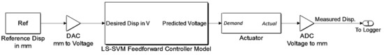
Figure 1.
Feed-forward control of the actuator utilizing the trained least-squares support-vector machine LS-SVM model.
2. Servo-Hydraulic Actuator Hysteresis
To provide a model for controlling actuators, it is necessary to examine the hysteresis behavior of the actuators. Hysteresis means lagging behind; the usage of the term in literature dates back to a century ago, when Alfred Ewing, the Scottish physicist, used this word [15]. Since then, it has been the collective name for a class of strongly nonlinear phenomena. Lagging in hysteretic systems usually has two different origins. It can occur by changing the internal state of the system or rate dependence. Unfortunately, the internal state change of the systems is not directly measurable; this property plays a decisive role and makes hysteresis a non-unique nonlinearity. Owing to this, hysteresis is considered a multiple-valued mapping in the literature.
Numerical Modeling of Servo-Hydraulic Actuators
To generate sets of data from the inputs and outputs of actuators, a numerical model of the actuator was simulated. For this purpose, a numerical model of a servo-hydraulic actuator presented in Qian et al. [16] was used. The model mostly considers the servo-valve flow and its controller, actuator pressure dynamics, and test specimen dynamics. The model consists of three transfer functions to simulate the servo valve, actuator dynamics, and test specimen [16]. In the model, Xd (reference or desired displacement) and X (feedback of the system or applied displacement) are the input and output of the model, respectively. There are five assumptions in this model, which are categorized in [16]:
- (1)
- Fluid properties are constant;
- (2)
- Servo valves are not saturated;
- (3)
- Supply pressure is much greater than the load pressure;
- (4)
- Friction force can be modeled as viscous damping;
- (5)
- The main stage spool opening is proportional to the pilot stage flow.
Qian et al. [16] identified parameters of the actuator, such as pilot stage valve flow, valve flow gains, pressure gain, piston area, piston leakage coefficient, effective actuator damping, and initial actuator mass. Among all of these parameters, the piston area is given by the manufacturer (in this model, 497 mm2), and the internal controller’s proportional gain can be adjusted through the controller’s user interface. All remaining parameters have been identified in their study. More details of the model and parameters as well as the block diagrams of the actuator are presented in Reference [16].
In this study, a numerical model of the actuator whose parameters have been identified by Qian et al. [16] was created using Matlab Simulink®, and specimen stiffness was chosen to be 67.6 kN/m.
3. Least-Squares Support-Vector Machine (LS-SVM)
Supervised learning systems that analyze data and recognize patterns are known as support-vector machines (SVMs), which are used for classification (machine learning) and regression analysis. Support-vector machines (SVMs) were introduced in 1992 [17]. In this method, one maps the data into a higher dimensional input space and constructs an optimal separating hyperplane in this space (more information is available in the “Least-Squares Support-Vector Machine” by Suykens and Vandewalle) [18]. The soft margin classifier was introduced by Cortes and Vapnik [19]; then, the algorithm was extended to the case of regression by Vapnik et al. [20]. SVMs can be used as linear and nonlinear classifiers as well as function approximators. Actually, they are known as sparse kernels. The standard form of the SVM adopts an ε-insensitive loss function, while LS-SVMs utilize a squared loss function. In this version, one finds the solution by solving a set of linear equations instead of the convex quadratic programming (QP) problem for classical SVMs. Least-squares SVM classifiers were proposed by Suykens and Vandewalle [18]. LS-SVMs are a class of kernel-based learning methods. The main relations utilized to estimate the static function by LS-SVMs are presented in the following. First, the input data maps z to a high-dimensional feature space by LS-SVM and approximates the output f through a linear regression using Equation (1):
where w is a weight vector, b is the bias, and ψ(0) indicates a nonlinear mapping from the input space to a feature space. Equation (1) approximates the unknown nonlinear function f = f(z), assuming the training data set , where N represents the number of training data sets.
The derivation of the following resulting LS-SVM model for function approximation is presented in Reference [21]:
where αm and b are the solution of the linear set. The solution is unique if the Mercer kernel is utilized [22]. In this case, the Gram matrix Ω is positive definite.
The kernel function’s role is to avoid the explicit definition of the mapping ψ(0). The simplest form of kernels is
converting LS-SVM to a linear regression. The Radial Base Function (RBF) kernel, which is widely utilized in nonlinear function estimation, is as follows:
where represents Euclidean distance and σ denotes the width parameter. Both aforementioned kernels are Mercer kernels; therefore, αn and b can be uniquely determined for the pre-assigned hyper-parameters σ and γ.
The numerical modeling of hysteretic behavior is challenging. To overcome this problem, Joghataie and Farrokh [23] proposed a Prandtl neural network based on the Prandtl–Ishlinskii operator. Prandtl proposed the modeling of the elastic–plastic behavior of materials with the following relation [24]:
In Equation (5), w(r) = the density function, εr = the elastic–plastic (stop) operator, r = yield point of the stop operator, x(t) = the input signal, and f(t) = the output signal. For positive real values, the integration over r can be defined. Equation (5) is known as the classical Prandtl–Ishlinskii model, which is also named the stop operator. The output is calculated by weighted summation of an immense number of stop operators. Detailed descriptions of the main relations utilized to estimate the static function by LS-SVMs are presented in Farrokh [25].
Readers are encouraged to refer to Farokh [25], Joghataei and Farrokh [23], and Sharghi et al. [21] for comprehensive descriptions of PNN (Prandtl neural network) and its applications.
LS-SVM Hysteresis Model
In this paper, the preliminary model proposed by Farrokh [25]—which is inspired by Preisach hysteresis, which contains a discrete hysteresis memory and multivariate function—is enhanced, and a new version for feed-forward controlling of hydraulic actuators is introduced. At first, Farrokh’s model [25] converts hysteresis into one-to-one mapping using stop operators (classical hysteresis operators); then, the converted mapping is learned by an LS-SVM. Details of the model can be seen in Figure 2.
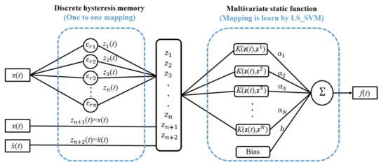
Figure 2.
LS-SVM hysteresis model architecture.
The discrete hysteresis memory part consists of n stop operators with distinct threshold values r1, r2, …, rn. These threshold values are assigned according to the equation below, where max is the maximum of the input signal absolute values.
In this study, an LS-SVM was chosen for modeling the second part (multivariate static function) to estimate the memoryless function (εr). Compared with neural networks, LS-SVMs take advantage of the error functions with a unique global minimum regarding their weights. Training of the LS-SVM would be done in one step with pre-assigned hyper-parameters γ and σ. The high generalization ability of the model relies on the appropriate tuning of these hyper-parameters. The tuning process is performed in two successive stages: (1) Coupled Simulated Annealing (CSA) [26] determines suitable values for the hyper-parameters, and (2) the Nelder–Mead simplex algorithm [27] uses these previous values as starting values in order to perform a fine-tuning of the hyper-parameters. Afterward, the training of the LS-SVM is done with the optimum hyper-parameters on the training data. The tuning and training procedures were implemented by utilizing the MATLAB LS-SVMlab Toolbox (Version 1.8) [28].
4. LS-SVM Hysteresis Model for the Servo-Hydraulic Actuator
4.1. Utilizing the LS-SVM Hysteresis Model for the Servo-Hydraulic Actuator
In this section, the procedure of training and testing of the LS-SVM hysteresis model for the servo-hydraulic actuator will be elaborated upon. Considering the characteristics of the actuator, the ranges of their displacement and frequency can be covered by utilizing proper excitations. Using the limits in the previous step, the proper excitations are used for the actuator. Thence, the suitable inputs for the input layer and stop operator are chosen. Finally, with the aid of MATLAB LS-SVMLab Toolbox (Version 1.8) [28], the training process is done. After that, if the results of the model’s anticipation of the input of the actuator from its output were satisfactory, then, the model should be tested by other excitations; otherwise, the excitation, input layer, or some tuning parameters in LS-SVMlab Toolbox should be modified. The steps for utilizing the LS-SVM hysteresis model for actuators are illustrated in Figure 3.
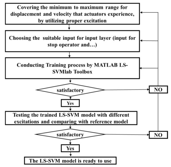
Figure 3.
Procedure of training and testing of the LS-SVM hysteresis model.
4.2. Performance Assessment of the LS-SVM Hysteresis Model for the Numerical Servo-Hydraulic Actuator
In this section, the capabilities of the LS-SVM hysteresis model for predicting the input voltage of the actuator for a given output displacement are evaluated. The most critical requirement for feed-forward hysteresis control is that the effect of the output of the system on the input should be known. Servo-hydraulic actuator hysteresis loops are categorized as rate-dependent hysteresis types. In rate-dependent hysteresis types, the output signal of the plant, X(t), depends on the rate at which the input signal, (t), changes. Figure 4 portrays the proposed version of the LS-SVM hysteresis model. For feed-forward hysteresis control, the LS-SVM model utilized is illustrated in Figure 4. Figure 5 portrays the flowchart of the required steps for evaluating the performance of the LS-SVM model for feed-forward controlling of actuators. In this study, (t) and X(t) are inputs for the Prandtl operator and (t) and X(t) are in the input layer, while the output layer contains V(t).
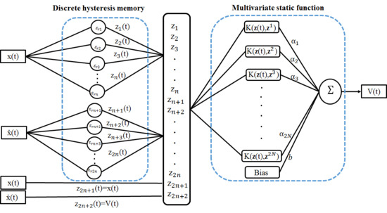
Figure 4.
Architecture of the inverse LS-SVM hysteresis model for the servo-hydraulic actuator.
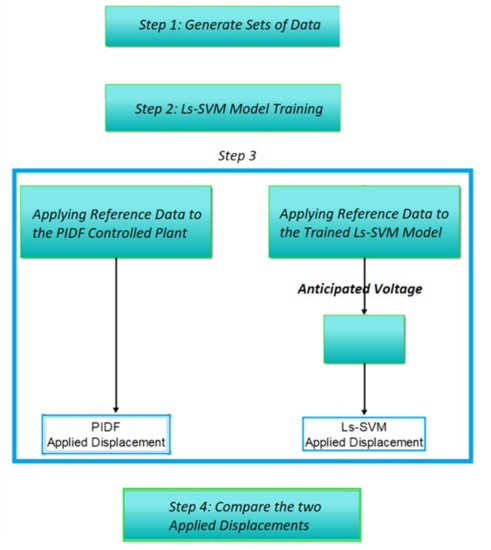
Figure 5.
Flowchart of the performance assessment of the LS-SVM feed-forward controller.
The reference model with the PIDF (Proportional-Integral-Derivative-Feed-forward) controller proposed by Karami Mohammadi et al. [29] was utilized for the assessment of the LS-SVM model. The controller that was used in the Qian et al. is an inner-loop P-controller (see Figure 6a) which works in conjunction with another outer-loop controller to have the best performance. However, in this study, the PIDF controller presented in Mohammadi et al. [29] was chosen for the control of the servo-hydraulic system (see Figure 6b) instead, since it is a well-known methodology used by most commercial hydraulic controllers and is also relatively simple to tune.
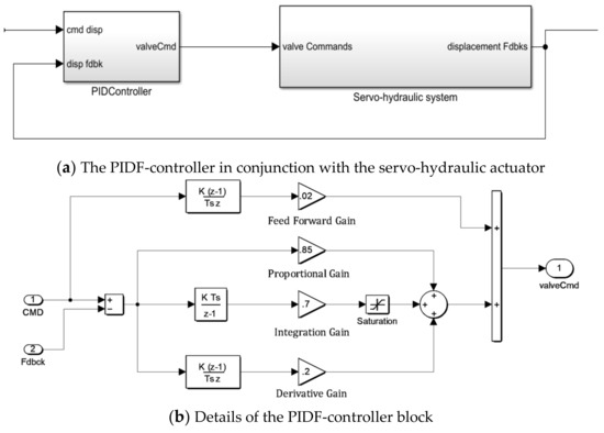
Figure 6.
Proportional-Integral-Derivative-Feed-forward (PIDF)-controller in conjunction with the servo-hydraulic actuator and the details.
For the LS-SVM, there was no need to define the network architecture and the number of neurons (which was taken as five); therefore, the training procedures were done only once. To compare the performances of the two controlling methods, the difference of the computed/predicted displacements of the two methods normalized by the maximum of the reference displacement was calculated. The normalized error can be expressed as follows:
where XREF,i and XMODEL,i represent the actuator displacement in Step i in the reference model, and in the considered system, respectively.
According to Figure 5, to assess the ability of the LS-SVM model for feed-forward controlling of actuator (predicting the required voltage for the servo valve (input voltage)), the first step was to create sets of inputs and outputs of the numerical actuator. For this purpose, different sets of pure sinusoidal and incremental-amplitude sine waves as the input voltages were generated. Then, the generated voltages were fed into the actuator without the controller, and the corresponding displacement was logged (referred to as reference displacements). Table 1 represents the sets of data prepared for the training and performance assessment of the LS-SVM feed-forward controller.

Table 1.
Input voltages.
Then, using different sets of input voltages and reference displacements, three different LS-SVM models were trained. Each model was then tested for other datasets with the same frequency as the training data. The properties of the trained models are presented in Table 2.
Table 2.
LS-SVM model properties.
In Step 3, the reference displacements obtained in Step 2 were set as the desired displacement of the PID-controlled actuator, and the applied displacement was logged. In addition, the trained LS-SVM models were tested for the datasets. Figure 7 shows the block diagram of the PID-controlled and LS-SVM-controlled plant.
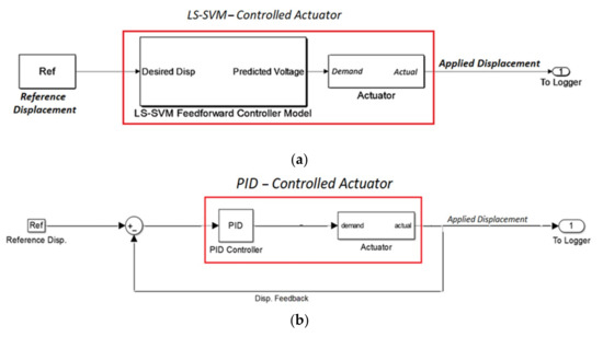
Figure 7.
Block diagrams of the models used for Step 3; (a) LS-SVM-controlled plant, (b) PID-controlled plant.
Finally, the applied displacements of the two methods were compared to the reference displacements. In addition, the normalized error of each method was plotted.
Results and Discussion
Model 1 was trained using Data #1 and Data #5; then, Data #2, Data #3, and Data #4 were utilized for testing the trained LS-SVM model. The results of the normalized errors of the two methods of controlling the actuator (PID and LS-SVM feed-forward) are depicted in Figure 8, Figure 9 and Figure 10.
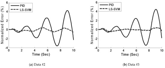
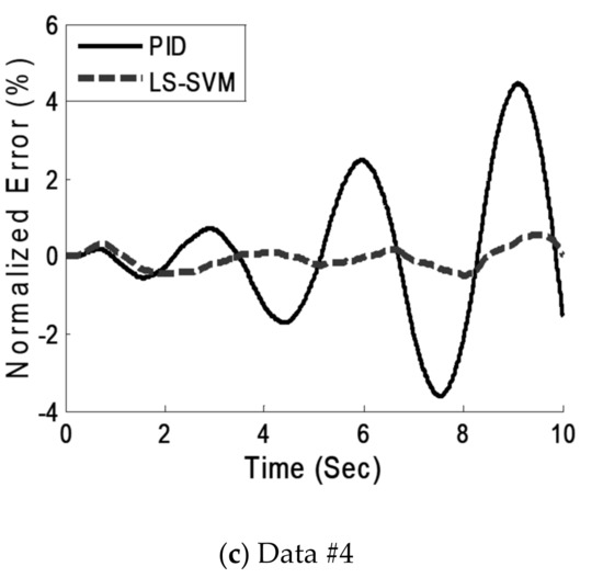
Figure 8.
Comparison of the normalized errors of Model 1 in different tests.
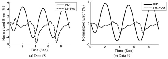
Figure 9.
Comparison of the normalized errors of Model 2 in different tests.
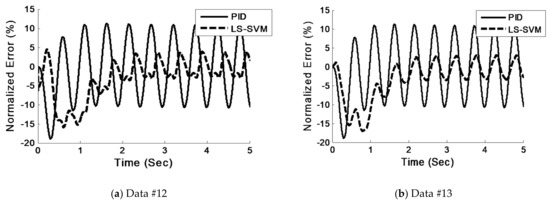
Figure 10.
Comparison of the normalized errors of Model 3 in different tests.
Model 2 was trained using Data #7 and Data #10. The Data #8 and Data #9 were utilized for testing the trained LS-SVM model. The results of the comparison of the normalized errors of the two methods of controlling the actuator (PID and LS-SVM feed-forward) are depicted in Figure 9.
Model 3 was trained using Data #11 and Data #14. The Data #12 and Data #13 were utilized for testing the trained LS-SVM model. The results of the comparison of the normalized errors of the two methods of controlling the actuator (PID and LS-SVM feed-forward) are depicted in Figure 10.
Comparing the applied displacement of the LS-SVM-controlled model with that of the PID-controlled plant, it can be seen that the LS-SVM-controlled plant shows great ability in predicting the input voltage in the training area. The normalized error of the LS-SVM-controlled plant is limited to 2% in most cases in the training zone. The values of normalized errors of PID-controlled plants in all cases are above those of the LS-SVM-controlled plants, confirming the better performance of the feed-forward LS-SVM controller.
As the simulation time goes on, the normalized error values are decreased, so the steady state of the error was reported and used in this study. The maximums of the steady states of the normalized error values in each test are tabulated in Table 3. In addition, the average error of the models is calculated. It can be seen that the maximum of the steady states of the normalized error of the models in the training zone is limited to 5%.
Table 3.
Normalized error of trained models.
4.3. Examining the Hysteresis Behavior of a Real Servo-Hydraulic Actuator
To examine the efficacy of the proposed method in practice, a database for training the LS-SVM was created using the HIFI-J servo-hydraulic actuator of the KNTU’s Structural and Earthquake Engineering Laboratory (KSEEL). For this purpose, the actuator HIFI-J (Quiri), which is illustrated in Figure 11, was utilized with no specimen attached. The actuator has a stroke of 300 mm (±150 mm) and a nominal maximum speed of 0.5 m/s at the frequency of 0.8 Hz. The maximum frequency of the actuator is limited to 5 Hz. The actuator’s characteristics are summarized in Table 4. In addition, the operational diagram of the actuator is depicted in Figure 12.
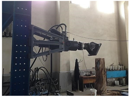
Figure 11.
Servo-hydraulic actuator.
Table 4.
Characteristics of the HIFI-J actuator.
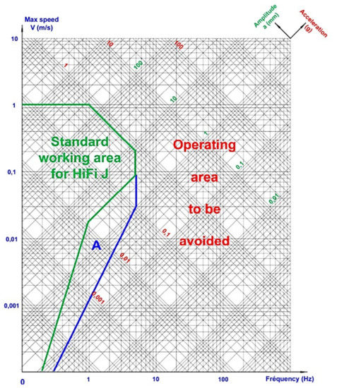
Figure 12.
Operational diagram of the actuator.
The main parts of a servo-hydraulic actuator can be expressed as follows:
- Hydraulic power unit (HPU)
- Manifold
- Servo valve
- Actuator
- Sensors (including load cell and LVDT (Linear variable differential transformer))
- Digital Controller
Each of these has a certain task during the test procedure. The controller gets the digital reference displacement in mm () and converts it to the analog reference voltage () (D/A (Digital/Analog) conversion). Then, comparing the reference voltage with the feedback voltage of the LVDT, it calculates the error value in volts. Afterward, using a P controller and multiplying the error value by 4.0, it sends the voltage to the servo valve (Commandvoltage) to achieve the desired displacement. Figure 13 plots the implemented block diagram of the actuator’s controller, written in LabWindows® by the Quiri industrial group.
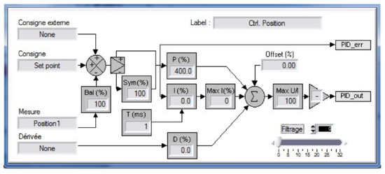
Figure 13.
Block diagram of the Quiri PID controller.
To create sets of input voltages and output voltages (feedback) of the actuator, a set of sinusoidal signals varying in amplitude and frequency was formed. Table 5 represents the defined protocols for generating the database. The reference signals were applied to the plant (P-Controlled Actuator) and the reference displacement and feedback displacement were logged at a frequency of 1000 Hz. The block diagram of the test procedure was drawn using Simulink® and is presented in Figure 14.
Table 5.
Displacement protocols.
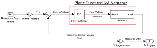
Figure 14.
Schematic view of the control system.
As was mentioned before, the reference and feedback displacement must be converted to the corresponding voltages. Then, using the P controller formulation presented below, the input voltage of the actuator was obtained:
where Vref is the reference voltage in volts, Vfdbk is the feedback voltage in volts, and P is the proportional gain of the controller, as can be seen in Figure 15. Figure 15 compares the input and feedback voltage of a sinusoidal output with an amplitude of 20 mm and frequency of 1 Hz.
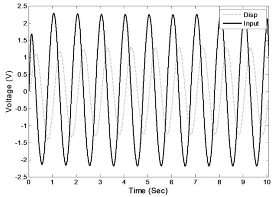
Figure 15.
Comparison of the input voltage and the corresponding sinusoidal output voltage of the plant.
Experimental errors are expected to contaminate the results of a simulation. The errors in experimental measurements can be reduced by proper tuning and calibration of test equipment and using high-performance instrumentation. However, it is virtually impossible to entirely eliminate all experimental errors; numerical procedures are often necessary in order to reduce their effects [10]. Although the data acquisition system implemented in the controller of the actuators has a 16 bit analog-to-digital converter (ADC) which significantly reduces the error, other environmental situations have negative effects on the logged data. In training LS-SVMs, even small errors can be propagated during the processing and can significantly affect the simulation results, yielding inaccurate outcomes. In this study, to reduce the noise of the gathered data and to reduce the spikes in the derivatives of data, all data were filtered using a Butterworth band-pass filter with the frequency band of 0.1 to 10 Hz in Matlab, Simulink®. Figure 16, Figure 17, Figure 18 and Figure 19 compare the filtered data with the original data; in addition, the derivatives of the two signals (filtered and original) are compared.
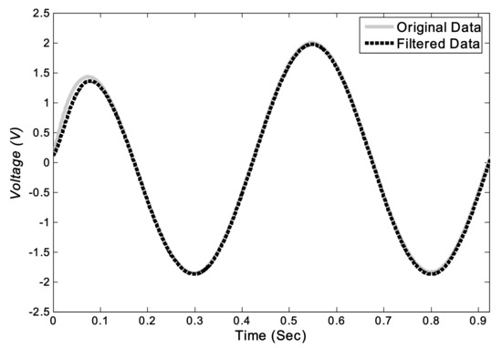
Figure 16.
Comparison of the original and filtered input voltages for Amp = 20 mm and Freq = 2 Hz.
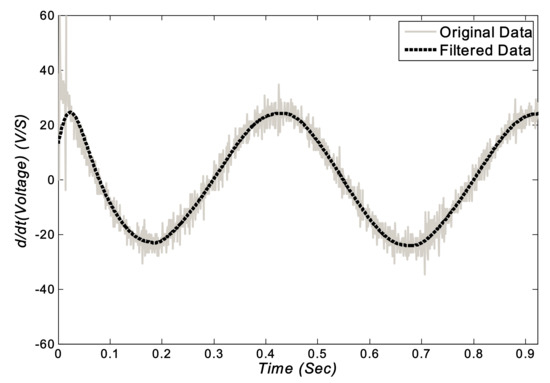
Figure 17.
Comparison of the derivatives of the original and filtered input voltages for Amp = 20 mm and Freq = 2 Hz.
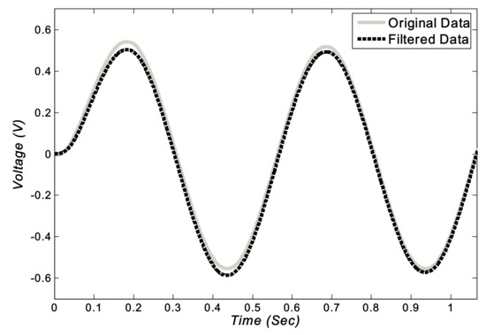
Figure 18.
Comparison of the original and filtered feedback voltages of the actuator’s LVDT for Amp = 20 mm and Freq = 2 Hz.
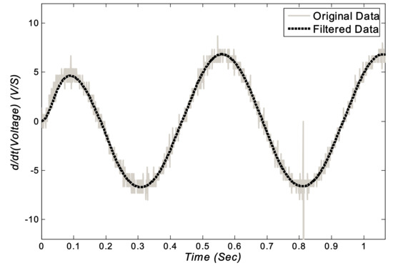
Figure 19.
Comparison of the derivatives of the original and filtered feedback voltages of the actuator’s LVDT for Amp = 20 mm and Freq = 2 Hz.
With sets of filtered input and output voltages of the actuator, LS-SVM models were trained to anticipate the input voltage of the actuator using the given output voltage. The LS-SVM model relies on the input voltage, feedback voltage, and the derivatives of the two mentioned signals to execute a reliable numerical model for predicting input voltages.
4.3.1. Sensitivity Analysis
In the current study, the LS-SVM network was trained for a given frequency using two different amplitudes. After that, it was tested for other amplitudes, with the same frequency with which the LS-SVM model was trained. Several LS-SVM models were trained using different sets of data. To reach an optimal LS-SVM model, a sensitivity analysis was carried out for the kernel type and number of neurons of the proposed LS-SVM network. Table 6 indicates the model properties and training material of each model.
Table 6.
LS-SVM model properties.
Kernel Type
To select a proper kernel type in this study, two models, Model 2 and Model 8, which are completely the same except that Model 8 uses the kernel type of RBF, were trained. Comparing the results of the two models indicates that although the RBF kernel type is capable of simulating its training data more precisely, the model was unable to predict other excitations as well. Figure 20 shows the comparison of the simulation outputs of the two models.
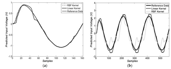
Figure 20.
Comparison of the results of Model 2 and Model 8 when (a) tested with trained data; (b) tested with Data #10.
It is evident that outputs of the model utilizing the linear kernel type are in a better agreement with that experimental data than those of the model with the RBF kernel type.
Number of Neurons
Four models (Models 2, 5, 6, and 7) have the same properties, except the number of neurons. The numbers of neurons vary from 10 to 100. A comparison of the results of the four models in predicting their training data, Figure 21, indicates that, as the number of neurons increases, high-frequency errors appear in the signal, and the computational efforts increase significantly. However, in these cases, the model with 10 neurons shows overshoot error to some extent; the models with 50 and 100 neurons are in good agreement with the reference signal. With regard to the obtained results and based on an engineering judgment, the number of neurons was chosen to be 100.
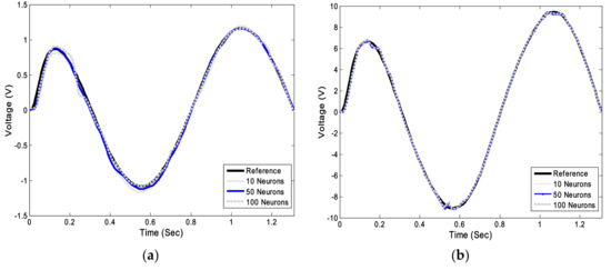
Figure 21.
Effect of the number of neurons on the response of the trained LS-SVM when (a) tested with Data #9; (b) tested with Data #14.
Finally, the linear kernel type and the number of 100 neurons were chosen for the LS-SVM models presented in Table 6. The results of the outputs of Model 1 to Model 4 are presented in Section 4.4.
4.4. Results and Discussion
To examine the accuracy of the trained models, the predicted input voltages of the models are compared to the reference input voltages obtained from experimental modeling. Figure 22, Figure 23 and Figure 24 depict the diagrams of the predicted input voltages and reference input voltages of all models. As can be seen, the predicted voltages are in a reasonable agreement with those of the references. However, there is a slight error in the predicted voltage. This error could be related to the experimental errors (noise) in the training data. It should be noted that, for a better visual comparison of the results of the comparison of the predicted voltage and the reference voltage, only the first three cycles of response are depicted in the figures below.
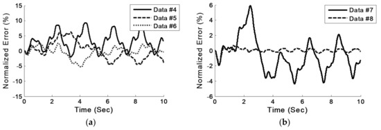
Figure 22.
Normalized error of Model 1 in different tests. (a) Tested with Data #4 to Data #6 (b) Tested with Data #7 and Data #8.
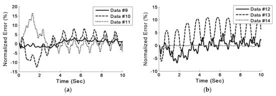
Figure 23.
Normalized error of Model 2 in different tests. (a) Tested with Data #9 to Data #11 (b) Tested with Data #12 to Data #14.
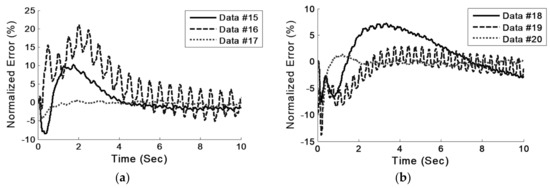
Figure 24.
Normalized error of (a) Model 3 and (b) Model 4 in different tests.
Comparing the results of controlling a real servo-hydraulic actuator using the proposed feed-forward controller with those of the PID controller shows the great ability of the LS-SVM controller. As can be seen in Figure 22, Figure 23 and Figure 24, the LS-SVM model could effectively control the servo-hydraulic actuator. As mentioned before, as the simulation time goes on, the normalized error values are decreased to a steady state. The values of the normalized errors are tabulated in Table 7. It can be seen that in all cases, the error values are limited to 10%, except for one.
Table 7.
Normalized errors of the trained models.
5. Conclusions
In this paper, an intelligent hysteresis model was proposed based on the learning capability of LS-SVM for open-loop feed-forward controlling of servo-hydraulic actuators. In the proposed method, a feed-forward-trained LS-SVM model is used in place of a feedback controller (PID controller). First, the ability of the LS-SVM method was examined numerically in Section 4.2; then, using a real 500 kN actuator at KSEEL with no specimen attached, sets of experimental data were generated for training the LS-SVM feed-forward controller. The outputs of the LS-SVM model affirm its ability in comparison with the PID controller. This study shows the efficiency of the proposed method and the capability of LS-SVM as a feed-forward controller. The results indicate that in most cases of this study, LS-SVM-controlled plants outperform PID-controlled systems. It was shown that LS-SVM has a great ability for learning the hysteresis behaviors of actuators; however, the presence of experimental noise could affect the accuracy of responses. To overcome the detrimental effects of the noise, a Butterworth band-pass filter with a frequency band of 0.1 to 10 Hz was used for filtering data. Comparing the two control strategies in terms of normalized error in both numerical and experimental plants confirms reasonable agreements between the responses of PID-controlled and LS-SVM-controlled plants. The normalized error values in the numerical simulation, in the absence of systematic noise, are limited to 5% in many cases; also, in the experimental simulation, in the presence of systematic noise, these are limited to 10%. The LS-SVM feed-forward controller could also be used in Virtual Hybrid Simulation (VHS) in place of the predictor corrector and PID controller. In the current study, sinusoidal waves were used for training and testing the proposed controller; however, for the sake of real-world problems, other excitations must be tested. The application of the LS-SVM feed-forward controller in VHS with other excitations remains for future rigorous studies. It should also be noted that the LS-SVM network training in this method must necessarily be performed by preliminary tests.
Author Contributions
Conceptualization, A.H.S., R.K.M. and M.F.; Methodology, A.H.S., R.K.M. and M.F.; Formal Analysis, A.H.S. and S.Z.; investigation, All; resources, All; data curation, All; Experimental Testing, S.Z. and A.H.S.; Writing – Original Draft Preparation, A.H.S. and S.Z.; Writing – Review & Editing, R.K.M. and M.F.; Visualization, A.H.S. and S.Z.; Supervision, R.K.M. and M.F.; Project Administration, R.K.M. and M.F. All authors have read and agreed to the published version of the manuscript.
Funding
This research received no external funding.
Conflicts of Interest
The authors declare no conflict of interest.
References
- Essa, M.E.-S.M.; Aboelela, M.A.S.; Hassan, M.A.M. Position control of hydraulic servo system using proportional-integral-derivative controller tuned by some evolutionary techniques. J. Vib. Control 2014, 22, 2946–2957. [Google Scholar] [CrossRef]
- Samakwong, T.; Assawinchaichote, W. PID Controller Design for Electro-Hydraulic Servo Valve System with Genetic Algorithm. Procedia Comput. Sci. 2016, 86, 91–94. [Google Scholar] [CrossRef]
- Sohl, G.A.; Bobrow, J.E. Experiments and simulations on the nonlinear control of a hydraulic servosystem. IEEE Trans. Control Syst. Technol. 1999, 7, 238–247. [Google Scholar] [CrossRef]
- Bonchis, A.; Corke, P.I.; Rye, D.C.; Ha, Q.P. Variable structure methods in hydraulic servo systems control. Automatica 2001, 37, 589–595. [Google Scholar] [CrossRef]
- Sirouspour, M.R.; Salcudean, S. On the nonlinear control of hydraulic servo-systems. In Proceedings of the 2000 ICRA Millennium Conference IEEE International Conference on Robotics and Automation. Symposia Proceedings (Cat. No. 00CH37065), San Francisco, CA, USA, 24–28 April 2000; pp. 1276–1282. [Google Scholar]
- Pedret, C.; Vilanova, R.; Moreno, R.; Serra, I. A refinement procedure for PID controller tuning. Comput. Chem. Eng. 2002, 26, 903–908. [Google Scholar] [CrossRef]
- Chang, W.-D.; Hwang, R.-C.; Hsieh, J.-G. A multivariable on-line adaptive PID controller using auto-tuning neurons. Eng. Appl. Artif. Intell. 2003, 16, 57–63. [Google Scholar] [CrossRef]
- Araki, M. PID Control, Control Systems, Robotics and Automation: System Analysis and Control: Classical Approaches II; EOLSS Publishers Co. Ltd.: Oxford, UK, 2002; pp. 58–79. [Google Scholar]
- Sung, S.W.; Lee, I.B. Limitations and countermeasures of PID controllers. Ind. Eng. Chem. Res. 1996, 35, 2596–2610. [Google Scholar] [CrossRef]
- Ahmadizadeh, M. On equivalent passive structural control systems for semi-active control using viscous fluid dampers. Struct. Control Health Monit. Off. J. Int. Assoc. Struct. Control Monit. Eur. Assoc. Control Struct. 2007, 14, 858–875. [Google Scholar] [CrossRef]
- Vinagre, B.M.; Monje, C.A.; Calderón, A.J.; Suárez, J.I. Fractional PID Controllers for Industry Application. A Brief Introduction. J. Vib. Control 2016, 13, 1419–1429. [Google Scholar] [CrossRef]
- Leang, K.K.; Zou, Q.; Devasia, S. Feedforward control of piezoactuators in atomic force microscope systems. IEEE Control Syst. Mag. 2009, 29, 70–82. [Google Scholar] [CrossRef]
- Zhang, X.; Wang, H. Research on Control Strategy for Inverter Based on Support Vector Machine. Trans. China Electrotech. Soc. 2005, 11, 44–48. [Google Scholar]
- Sharghi, A.H.; Karami Mohammadi, R.; Farrokh, M. Hybrid Simulation of a Frame Equipped with MR Damper by Utilizing Least Square Support Vector Machine. J. Numer. Methods Civ. Eng. 2018, 2, 58–66. [Google Scholar]
- Ewing, J.A.X. Experimental researches in magnetism. Philos. Trans. R. Soc. 1885, 157, 523–640. [Google Scholar]
- Qian, Y.; Ou, G.; Maghareh, A.; Dyke, S.J. Parametric identification of a servo-hydraulic actuator for real-time hybrid simulation. Mech. Syst. Signal Process. 2014, 48, 260–273. [Google Scholar] [CrossRef]
- Boser, B.E.; Guyon, I.M.; Vapnik, V.N. A training algorithm for optimal margin classifiers. In Proceedings of the Fifth Annual Workshop on Computational Learning Theory, Pittsburgh, PA, USA, 27–29 July 1992; pp. 144–152. [Google Scholar]
- Suykens, J.A.; Vandewalle, J. Least squares support vector machine classifiers. Neural Process. Lett. 1999, 9, 293–300. [Google Scholar] [CrossRef]
- Cortes, C.; Vapnik, V. Soft Margin Classifier. U.S. Patent 56,404,92A, 17 June 1997. [Google Scholar]
- Vapnik, V.; Golowich, S.E.; Smola, A.J. Support vector method for function approximation, regression estimation and signal processing. In Advances in Neural Information Processing Systems 9; Mozer, M.C., Jordan, M.I., Petsche, T., Eds.; MIT Press: Cambridge, MA, USA, 1997; pp. 281–287. [Google Scholar]
- Sharghi, A.H.; Mohammadi, R.K.; Farrokh, M. Neuro hybrid simulation of nonlinear frames using Prandtl Neural Networks. Proc. Inst. Civ. Eng. 2019. [Google Scholar] [CrossRef]
- Murphy, K.P. Machine Learning: A Probabilistic Perspective; MIT Press: Cambridge, MA, USA, 2012. [Google Scholar]
- Joghataie, A.; Farrokh, M. Dynamic analysis of nonlinear frames by Prandtl neural networks. J. Eng. Mech. 2008, 134, 961–969. [Google Scholar] [CrossRef]
- Visintin, A. Differential Models of Hysteresis; Springer: Berlin, Germany, 1994. [Google Scholar]
- Farrokh, M. Hysteresis simulation using least-squares support vector machine. J. Eng. Mech. 2018, 144, 04018084. [Google Scholar] [CrossRef]
- Xavier-de-Souza, S.; Suykens, J.A.; Vandewalle, J.; Bollé, D. Coupled Simulated Annealing. IEEE Trans. Syst. Man Cybern. Part B (Cybern.) 2010, 40, 320–335. [Google Scholar] [CrossRef] [PubMed]
- Nelder, J.A.; Mead, R. A simplex method for function minimization. Comput. J. 1965, 7, 308–313. [Google Scholar] [CrossRef]
- De Brabanter, K.; Karsmakers, P.; Ojeda, F.; Alzate, C.; De Brabanter, J.; Pelckmans, K.; De Moor, B.; Vandewalle, J.; Suykens, J.A.K. LS-SVMlab Toolbox User‘ Guide version 1.8; Katholieke Universiteit Leuven: Leuven, Belgium, 2011. [Google Scholar]
- Mohammadi, R.K.; Ghaffary, A.; Mohagheghian, K. Numerical Modeling of Dynamic Testing System for Structural Virtual Hybrid Simulation. In Proceedings of the 2nd International Conference on Civil, Architectural and Urban Management, Tehran, Iran, 16 August 2017. [Google Scholar]


© 2020 by the authors. Licensee MDPI, Basel, Switzerland. This article is an open access article distributed under the terms and conditions of the Creative Commons Attribution (CC BY) license (http://creativecommons.org/licenses/by/4.0/).