4.2. Experimental Results
For the experimental setup in
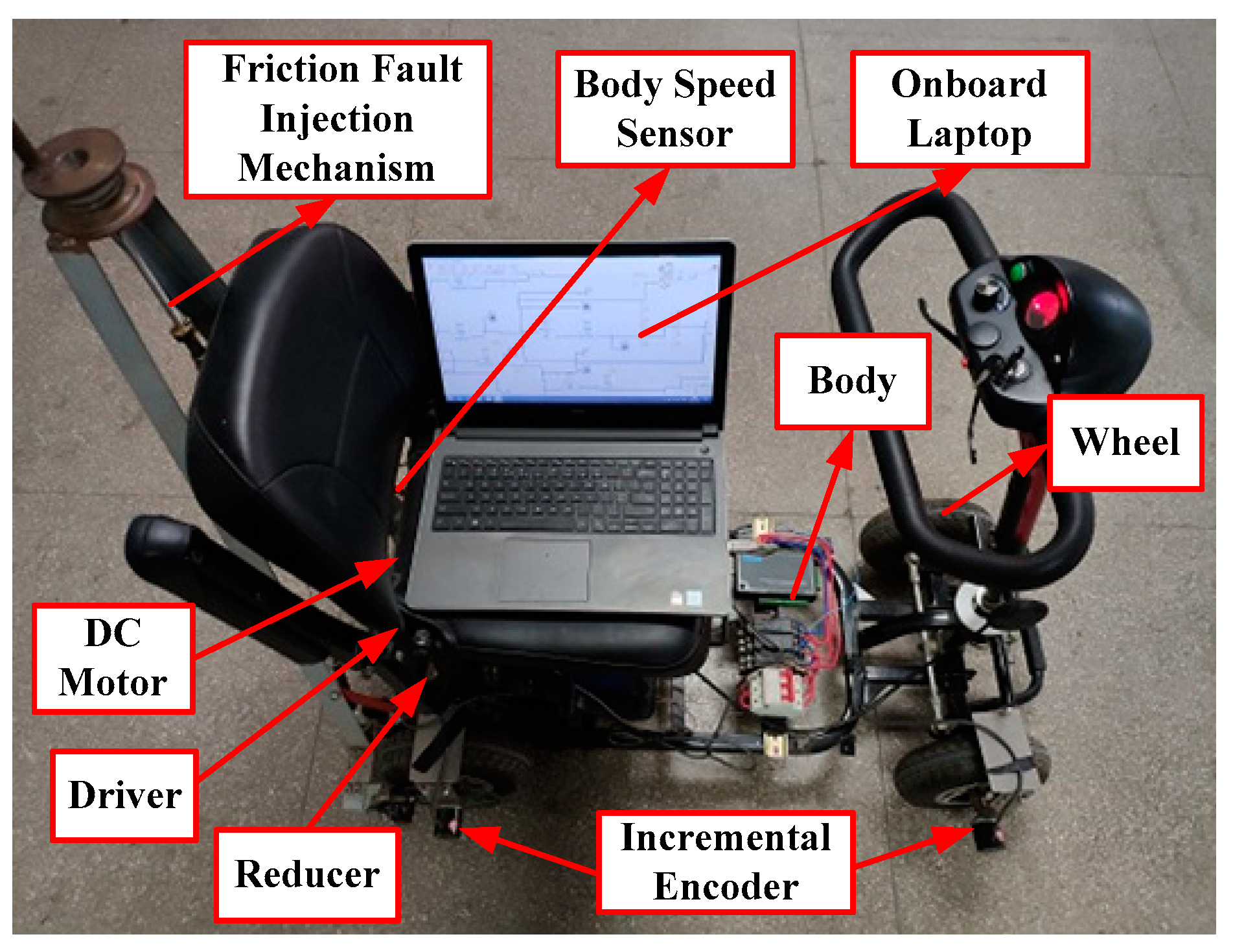
Figure 1, three sensors and motor are powered by two 12 V batteries. The sensors and associated hardware measures the scooter velocities and then send them to the onboard laptop via USB data acquisition card (Advantech USB 4711A) and LabVIEW software. The onboard laptop also provides power to the USB data acquisition card and sends command input signal to the motor driver. FDI is implemented by the standard LabVIEW module, while fault estimation and RUL prediction are conducted by utilizing the MATLAB script node in LabVIEW environment where the co-simulation between MATLAB and LabVIEW can be implemented online.
Two experiments under compound faults are conducted. The first one concerns an abrupt friction fault in
on the rear wheel and a monotonic intermittent sensor fault in
. A special mechanical arrangement in
Figure 1 is fabricated to introduce the friction fault in
. The mechanism consists of rotary disc, steel wire, and rubber sheet. The rotary disc can be manually rotated to drive the steel wire connected with the rubber sheet. The steel wire can control the distance between rubber sheet and the rear wheel. Under normal condition, the rubber sheet and the rear wheel are totally separated. When the rubber sheet is engaged with the rear wheel, the rear wheel friction is increased and the fault severity is determined by the rotation angle of the rotary disc. When the abrupt friction fault is injected, the rotation angle of the rotary disc under this fault condition is marked. For reference purpose, the abrupt fault value of
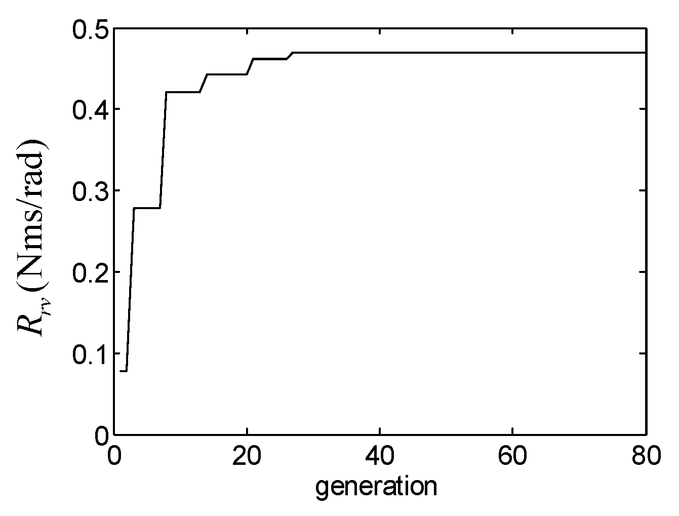
is needed and thus, the GA based fault identification (only suitable for the case of abrupt fault) is adopted, where only
is the unknown parameter and other parameter values are taken from
Table 3.
Figure 6 shows the identification result where the identified
= 0.469 Nms/rad.
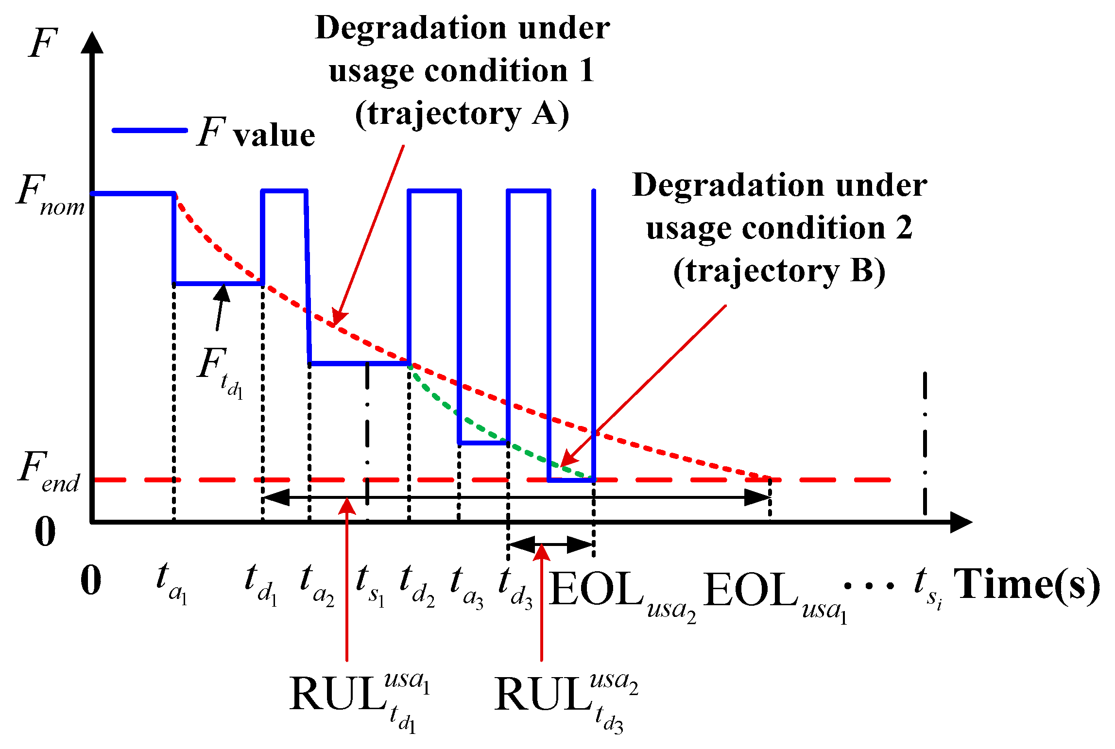
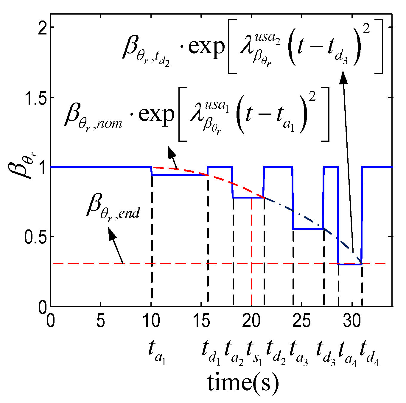
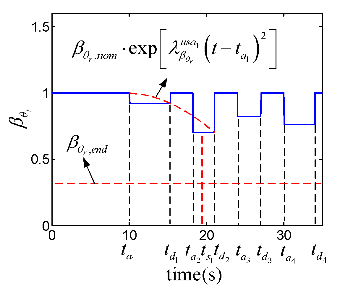
The intermittent fault profile is given in
Figure 7. The designed fault appearing and disappearing moments are
= 10 s,
= 15.56 s,
= 18 s,
= 21.16 s,
= 24 s,
= 27.08 s,
= 28.5 s,
= 30.94 s, and the fault values at the appearing interval are 0.94, 0.78, 0.55 and 0.3. The failure threshold
= 0.3. The input representing the usage condition is changed from 1 V to 1.2 V at
= 19.8 s. The degradation coefficient
under
and
under
. The designed RUL is 18.98 s under
and 3.86 s under
.
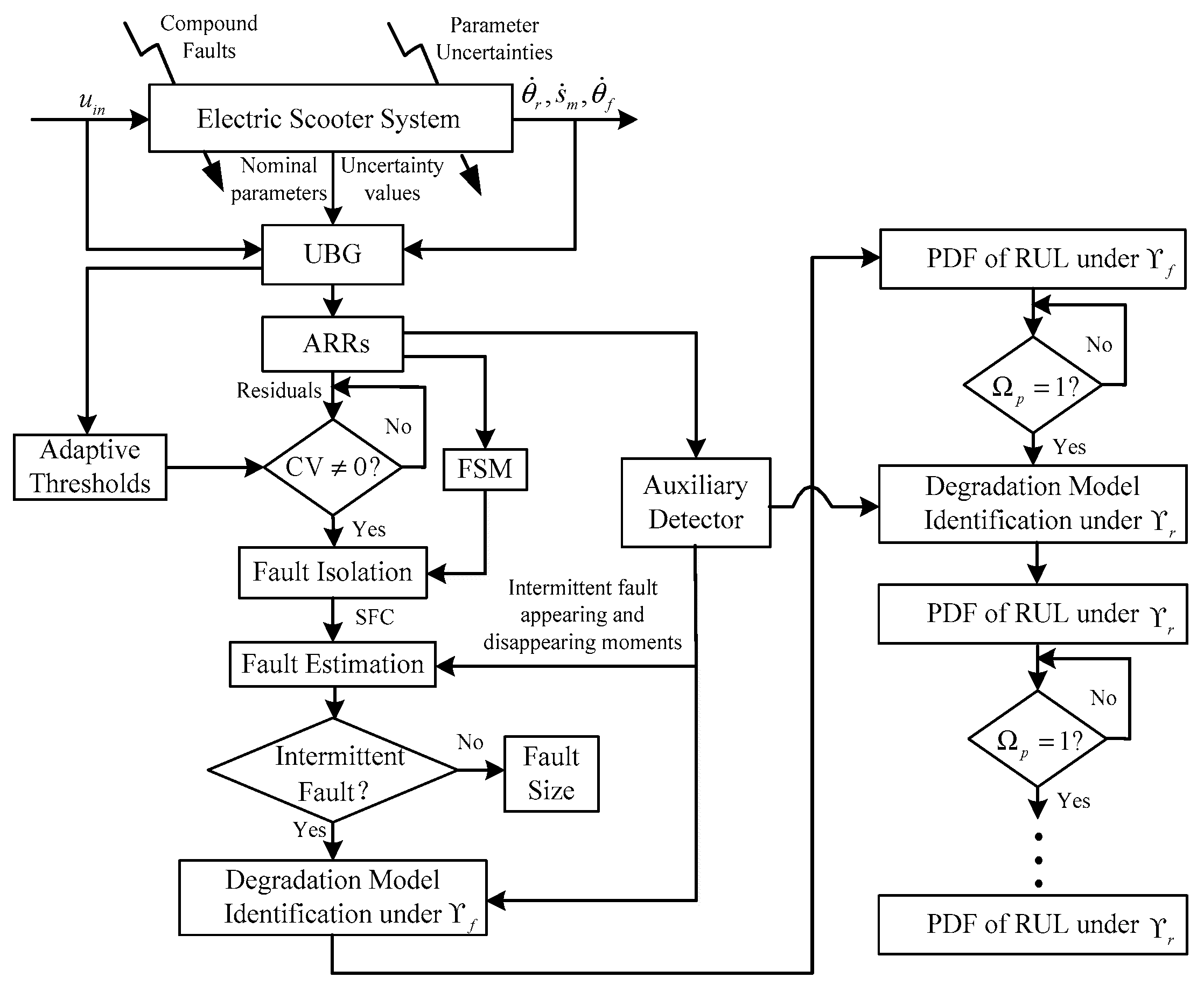
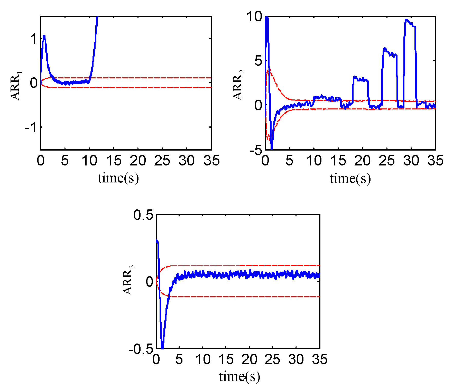
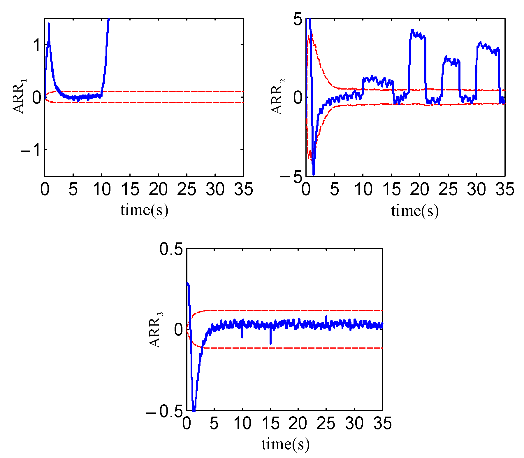
The residual responses are shown in
Figure 8. The nonlinear discrete model in (5) is obtained by discretizing the continuous model in (2)–(4) using Euler’s backward difference method. To guarantee the discrete model accuracy, the sampling time should be short enough. On the other hand, the sampling time must be long enough to assure the real time computation of the developed method. Thus, a tradeoff is made where the sampling time is chosen as 0.02 s. From
Figure 8, a CV = [1 1 0] is detected after 10 s and the SFC is
. After that, the fault estimation is activated where AEUKF, AUKF and UKF are employed for comparison purpose [
29]. The initial parameters for all filters are selected as
= diag(0.01, 0.01, 0.01, 0.01, 0.01, 0.01, 0.5, 0.3, 20),
= diag(0.01, 0.01, 0.01, 0.01, 0.01, 0.01, 0.01, 0.01, 0.01), and
= diag(0.2, 0.2, 0.2).
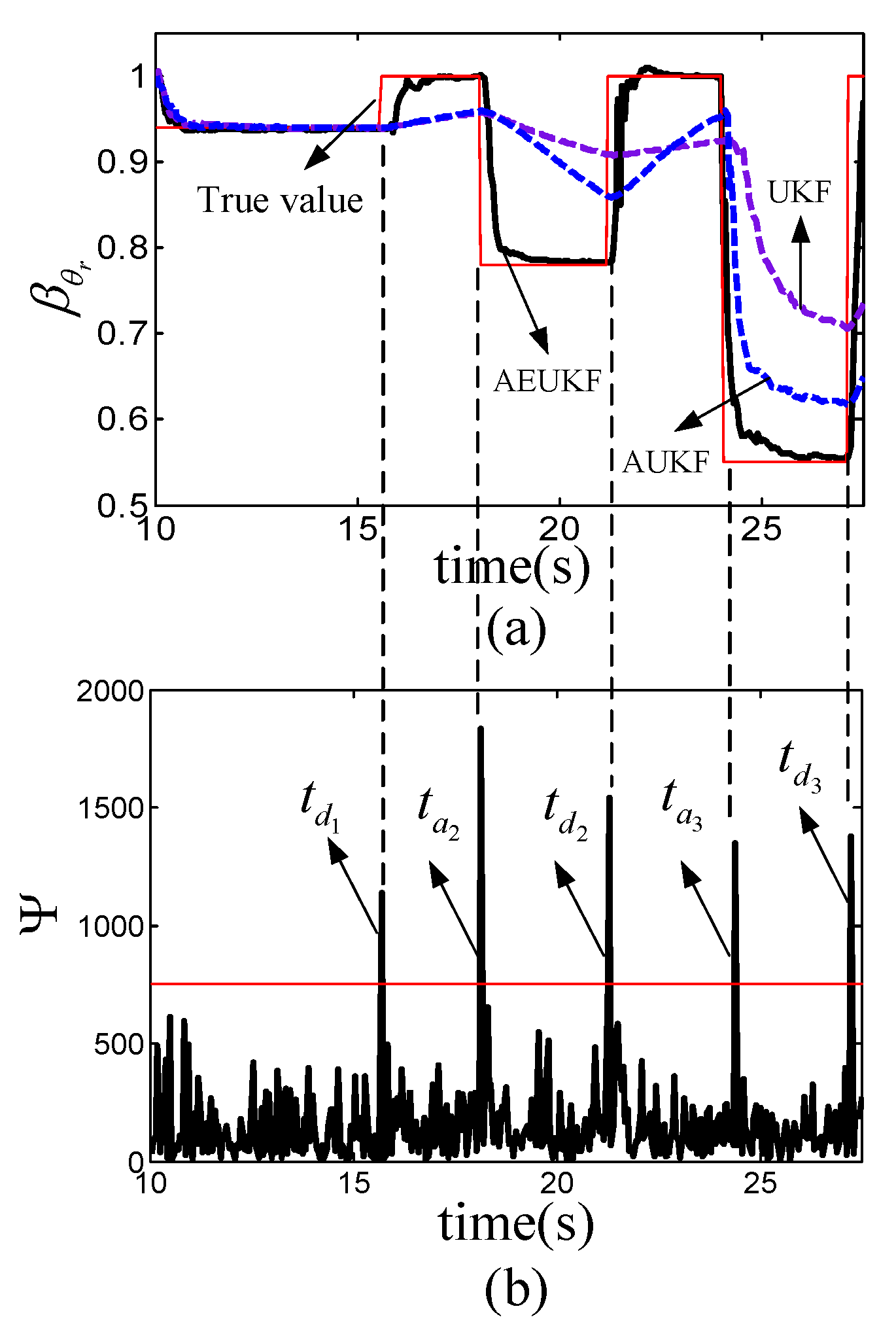
Figure 9a shows the estimate of
and
Figure 9b illustrates the response of
where the dashed line is the threshold of the auxiliary detector
. The
is calculated by the derivative function in LabVIEW. Since the choice of
in (6) is critical for the AEUKF, a set of experiments are conducted to choose
properly. It is found that the performance of sudden change tracking improves with the increase of
. However, when
τ increases beyond 5, poor tracking performances (i.e., large estimate fluctuations during sudden change instants and deteriorations in tracking error) occur. As a result,
is set to be 5. It is observed from
Figure 9a that UKF and AUKF do attempt to follow the step changes, but the convergence is too slow to track the true value before next sudden change occur. By contrast, the AEUKF can ensure the prompt tracking of the sudden changes by enhancing the posteriori state error covariance timely with the aid of the auxiliary detector
. The estimated values of
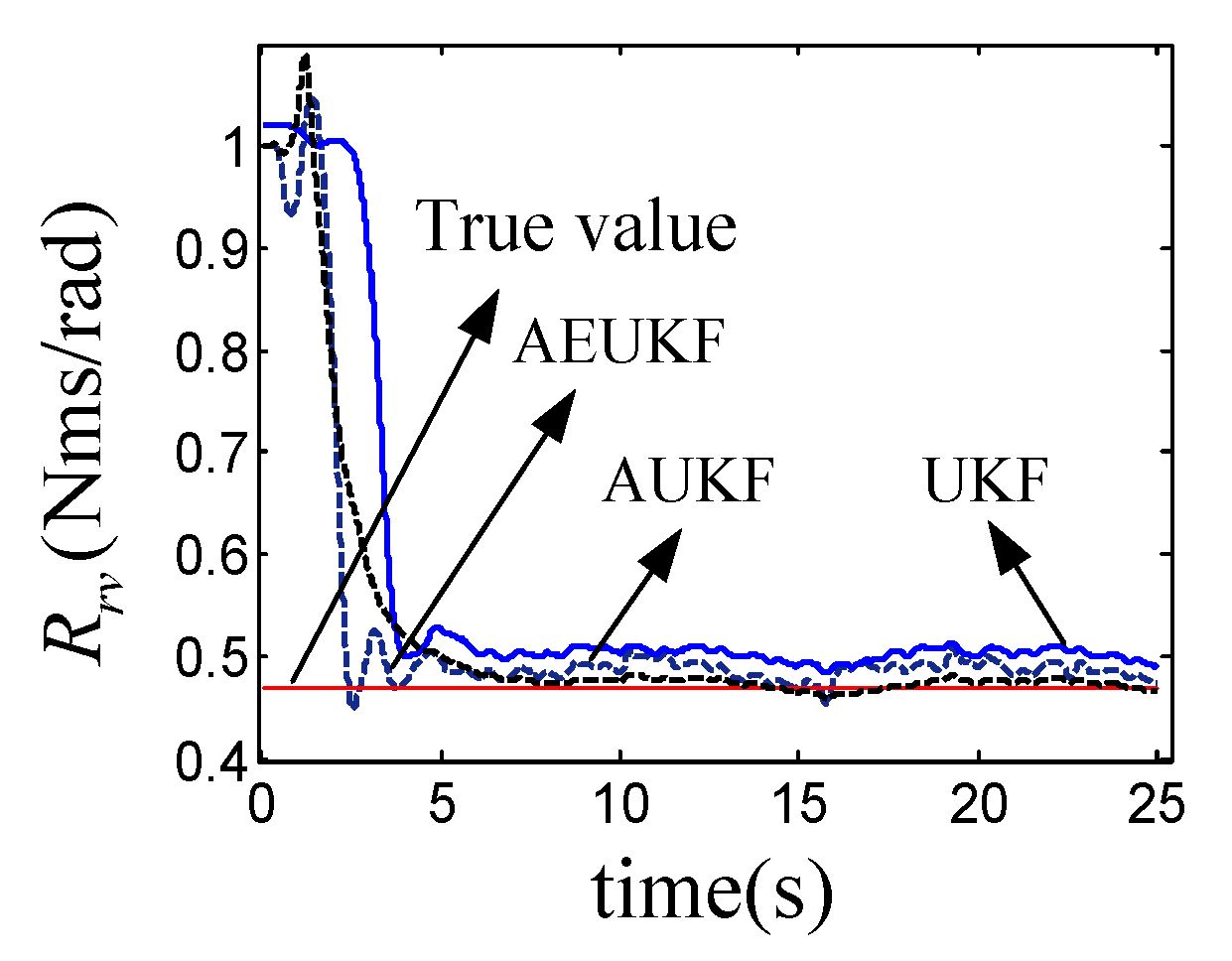
(shown in
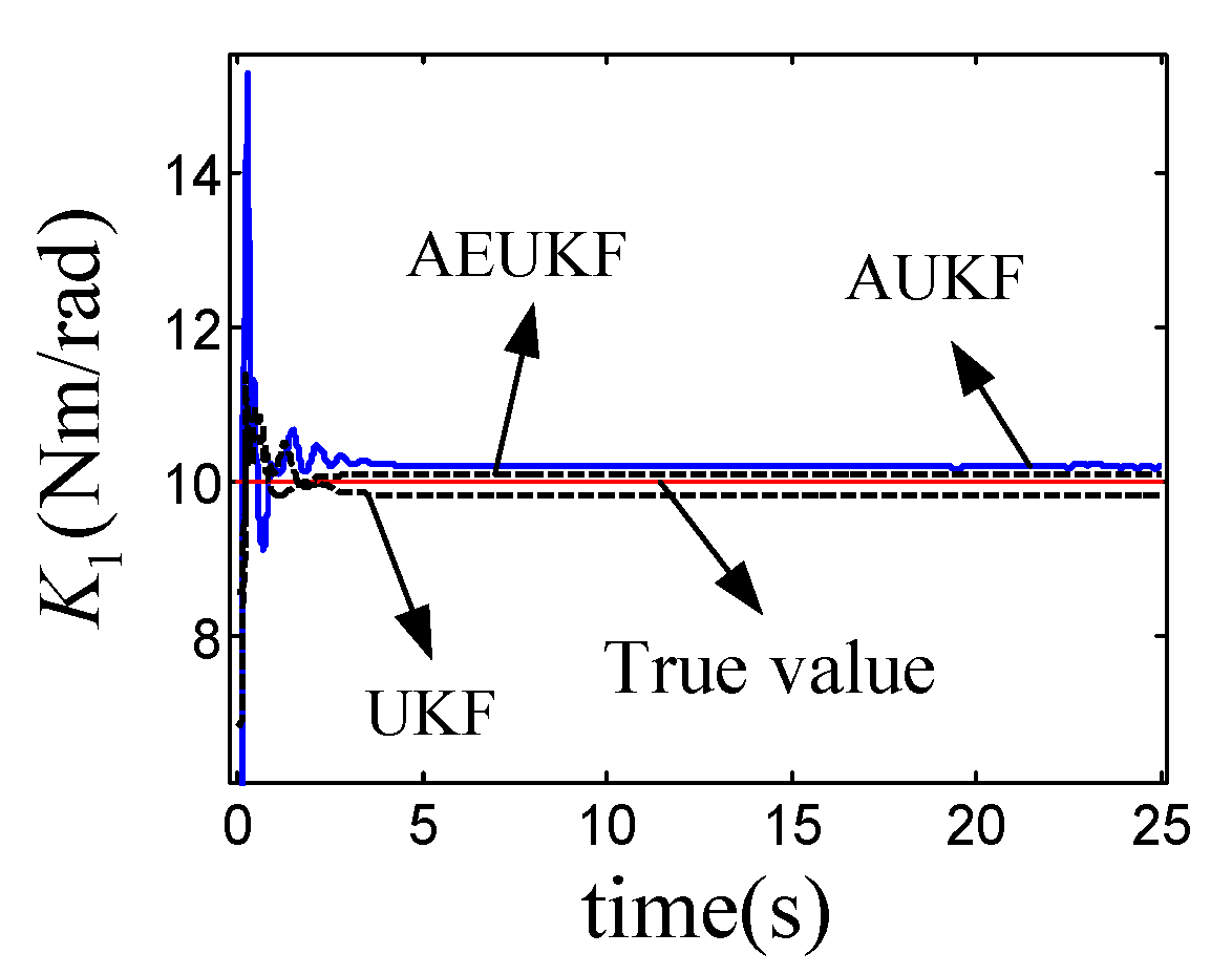
Figure 10) using AEUKF, AUKF and UKF, are 0.463 Nms/rad, 0.478 Nms/rad and 0.487 Nms/rad, respectively, which are close to the actual fault value (i.e., 0.469 Nms/rad). The estimated values of
(shown in
Figure 11) using AEUKF, AUKF and UKF, respectively, are 10.09 Nm/rad, 10.14 Nms/rad and 9. 85 Nm/rad, which are close to the nominal one (i.e., 10.02 Nm/rad). As the result, the
is excluded from the SFC. To show the average performance of fault estimation algorithms, more experiments (i.e., 6 sets of experiments) are conducted where the corresponding results are summarized in
Table 4. In the table,
,
, represents the time period between
and
. It was found that AEUKF and AUKF are superior to UKF, owing to the employment of the covariance matching technique.
Since the identified fault type of
is intermittent based on
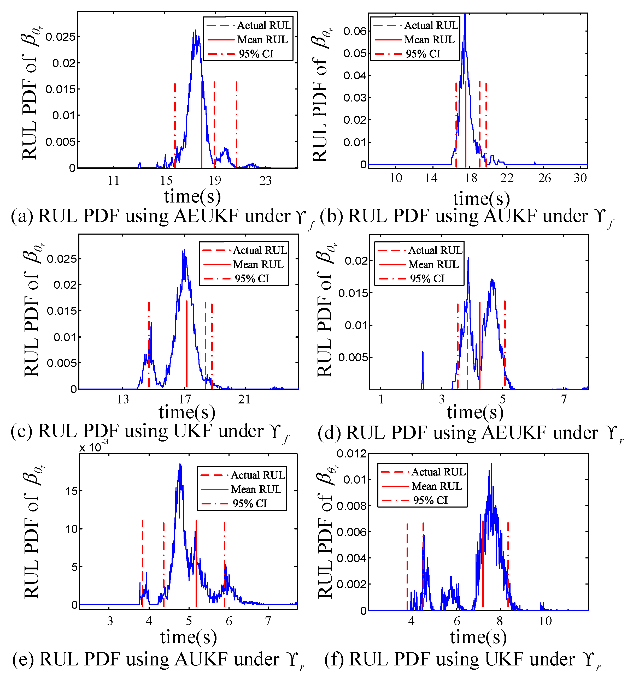
Figure 9a, the RUL is statistically predicted via the MCS method with M = 80.
Figure 12a–c, respectively, show the predicted RUL PDF based on the AEUKF, AUKF and UKF under
. The predicted mean RUL is 17.87 s for AEUKF, 17.83 s for AUKF, and 17.19 s for UKF. The actual RUL under
stays within 95% confidence interval (CI) for all filters. The AUKF and UKF are acceptable since no step change occurs before
(i.e., AUKF and UKF do not exhibit estimation latency before
). In order to quantitatively compare the prognosis performance of different methods, two metrics, i.e., relative accuracy (RA) for prediction accuracy and relative standard deviation (RSD) for prediction spread, are adopted [
14]. The performance results under usage 1 are given in
Table 5 where the metrics are expressed in percentages. From the table, it is observed that all methods yield good RA (i.e., over 90%) and RSD (i.e., under 10%). The performance of AUKF is almost the same as that of AEUKF. The slight decrease in performance of UKF is due to the difficulty of setting noise covariances.
After
, the usage condition is changed which causes the degradation to follow another trajectory as shown in
Figure 7. The prognoser is reactivated at
since
. From
Figure 9a, the AUKF and UKF cannot rapidly track the step changes which could adversely affect the subsequent degradation coefficient calculation and RUL prediction.
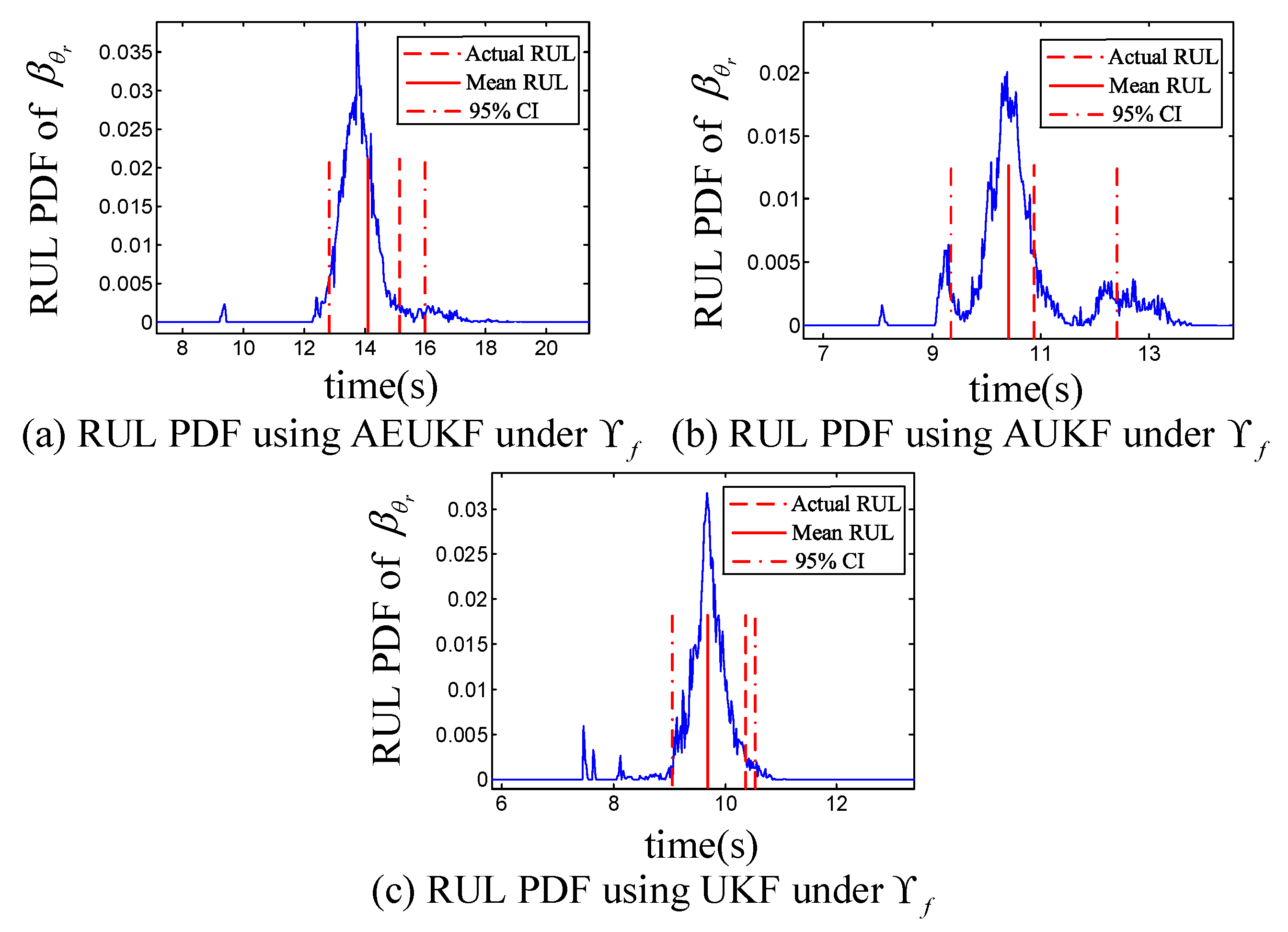
Figure 12d–f, respectively, illustrate the predicted RUL PDF using the AEUKF, AUKF and UKF under
. The predicted mean RUL is 4.21 s for AEUKF, which is close to the actual value (i.e., 3.86 s). The actual RUL falls inside the 95% CI. However, as expected, improper RUL predictions occur for AUKF and UKF, where the actual RUL falls outside the 95% CI. This is due to the overestimations of fault values which stems from the lack of ability to promptly track the sudden changes. As a result, the RUL predictions by the AUKF and UKF are not acceptable. The prognosis performances under usage 2 is shown in
Table 5 where the mark “
” in the entry indicates an unacceptable prediction metric.
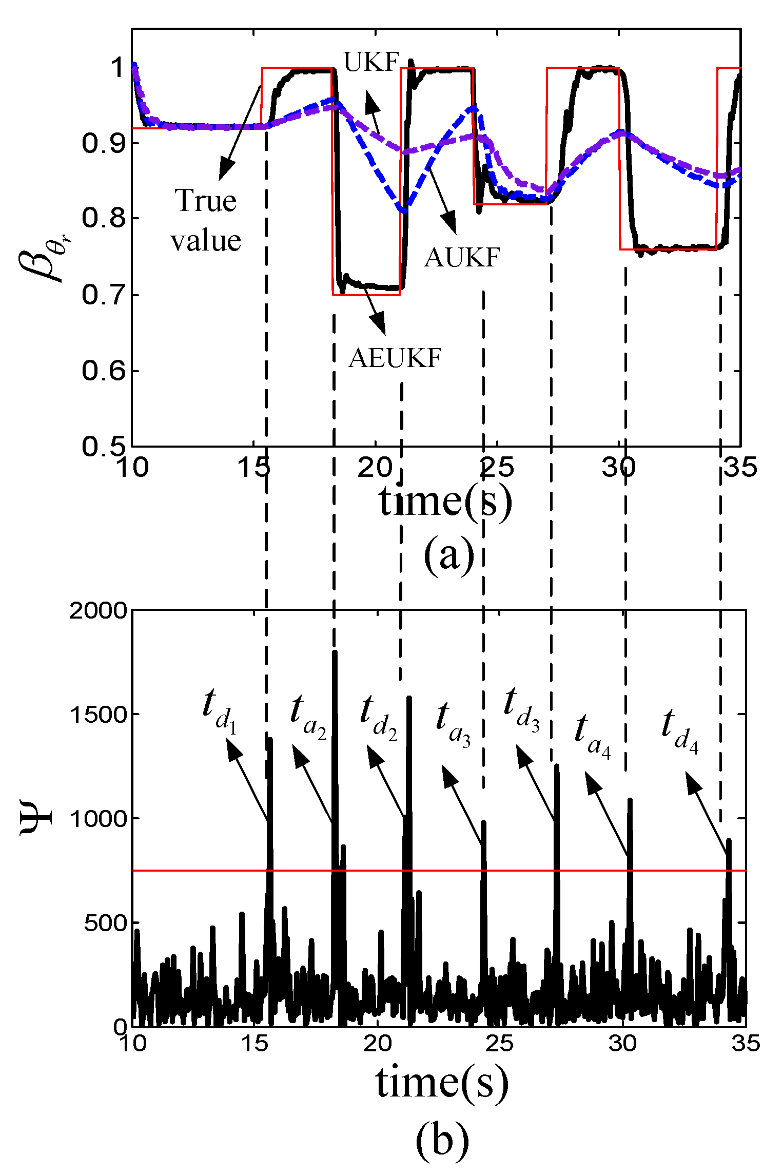
In the second experiment, an abrupt fault in
and a non-monotonic intermittent fault in
(whose profile is given in
Figure 13) are introduced. The designed fault appearing and disappearing moments are
= 10 s,
= 15.3 s,
= 19.2 s,
= 21 s,
= 24 s,
= 27 s,
= 30 s,
= 34 s, and the designed fault values at the appearing interval are 0.92, 0.7, 0.82 and 0.76. The failure threshold
= 0.3. The input representing the usage condition is changed from 1 V to 1.3 V at
= 19.7 s. The degradation coefficient
= −0.003 and the designed RUL is 14.8 s under
. The RUL under
is not available since the degradation is non-monotonic after
. The residual responses are presented in
Figure 14 where a CV = [1 1 0] is observed after 10 s and the resulting SFC is
. The fault estimation is then enabled where AEUKF, AUKF and UKF are adopted.
The estimation results are given in
Figure 15 where the AEUKF can ensure the timely tracking of sudden changes with the help of the auxiliary detector, but UKF and AUKF cannot work well. The estimated values of
using AEUKF, AUKF and UKF, are 0.461 Nms/rad, 0.447 Nms/rad and 0.445 Nms/rad, respectively. The estimated values of
using AEUKF, AUKF and UKF, respectively, are 9.94 Nm/rad, 9.91 Nms/rad and 10. 15 Nm/rad, which are close to the nominal one. Thus, the
is not a fault candidate and
is an abrupt fault.
Table 6 shows the average estimation results of 6 sets of experiments. In the table,
,
, represents the time period between
and
. From the
Table 6, it is observed that the AEUKF performs best among all methods.
The RUL prediction is carried out for
with M = 80.
Figure 16a–c, respectively, give the predicted RUL PDF based on the AEUKF, AUKF and UKF under
. The predicted mean RUL is 14.07 s for AEUKF, 13.84 s for AUKF, and 13.42 s for UKF. For all methods, the actual RUL remains within 95% CI. The prognosis performances of different methods are shown in
Table 5. It was observed that AUKF and AEUKF achieve similar performance since no sudden change occurs before
, while UKF performance decreases slightly. After
, the usage condition is changed where the degradation characteristic is non-monotonic as shown in
Figure 13. Thus,
is not satisfied and the prognoser will not be reactivated at
. As a result, the RUL of
under the new usage condition cannot be predicted.


