Predicting Ewe Body Condition Score Using Lifetime Liveweight and Liveweight Change, and Previous Body Condition Score Record

 , , ,
, , ,
Abstract
:Simple Summary
Abstract
1. Introduction
2. Materials and Methods
2.1. Farms and Animals Used and Data Collection
2.2. Statistical Analyses
2.3. Variable Selection, Model Building, and Validation
2.4. Model Performance Evaluation
3. Results
3.1. Correlation between all BCS and Liveweights
3.2. Linear Regression (Prediction of BCS)
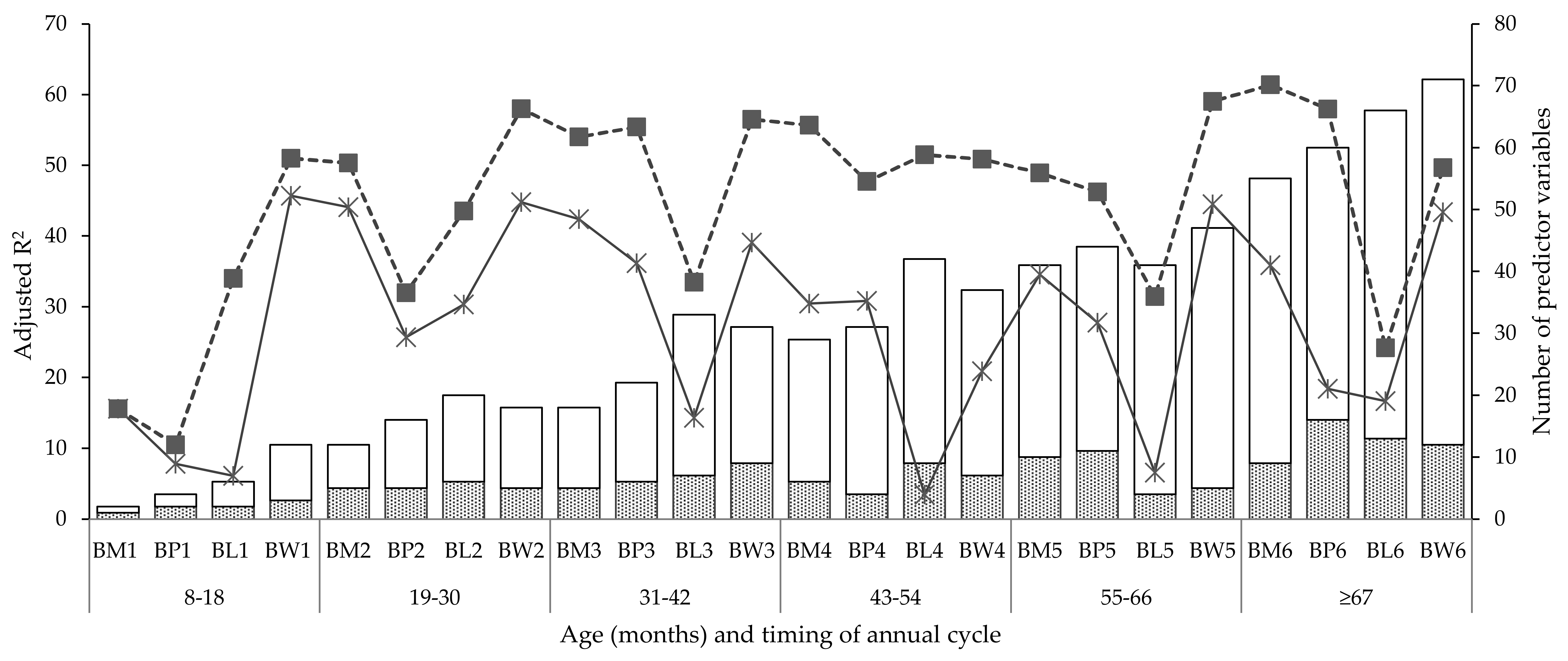
3.2.1. Coefficient of Determination (R2) and Number of Predictors
3.2.2. Prediction Error Metrics
4. Discussion
5. Conclusions
Author Contributions
Funding
Acknowledgments
Conflicts of Interest
Appendix A

| Predictor | BM1 | BP1 | BL1 | BW1 | BM2 | BP2 | BL2 | BW2 | BM3 | BP3 | BL3 | BW3 |
|---|---|---|---|---|---|---|---|---|---|---|---|---|
| WM1 | 0.04 | −0.02 | −0.01 | −0.02 | −0.01 | −0.01 | −0.02 | −0.01 | −0.01 | −0.01 | −0.01 | |
| WP1 | 0.04 | 0.02 | 0.01 | −0.03 | −0.03 | −0.03 | −0.01 | −0.01 | 0.01 | |||
| WL1 | −0.01 | −0.02 | 0.02 | 0.02 | 0.02 | −0.01 | ||||||
| WW1 | 0.05 | 0.01 | 0.01 | −0.01 | −0.01 | −0.01 | ||||||
| WM2 | 0.03 | 0.01 | 0.01 | −0.01 | −0.01 | |||||||
| WP2 | 0.03 | −0.01 | −0.01 | 0.01 | 0.01 | |||||||
| WL2 | 0.01 | −0.01 | −0.01 | |||||||||
| WW2 | 0.05 | 0.01 | ||||||||||
| WM3 | 0.04 | 0.01 | 0.01 | −0.01 | ||||||||
| WP3 | 0.05 | 0.01 | −0.01 | |||||||||
| WL3 | 0.02 | |||||||||||
| WW3 | 0.05 | |||||||||||
| WM4 | ||||||||||||
| WP4 | ||||||||||||
| WL4 | ||||||||||||
| WW4 | ||||||||||||
| WM5 | ||||||||||||
| WP5 | ||||||||||||
| WL5 | ||||||||||||
| WW5 | ||||||||||||
| WM6 | ||||||||||||
| WP6 | ||||||||||||
| WL6 | ||||||||||||
| WW6 | ||||||||||||
| Intercept | 1.40 | 2.14 | 2.6 | 1.27 | 1.33 | 1.62 | 2.26 | 1.26 | 1.69 | 1.26 | 1.94 | 1.84 |
| Adjusted R2 | 14.1 | 8.19 | 6.2 | 45.4 | 38.4 | 25.5 | 24.8 | 36.4 | 38.7 | 38 | 14.9 | 48.9 |
| Predictor | BM4 | BP4 | BL4 | BW4 | BM5 | BP5 | BL5 | BW5 | BM6 | BP6 | BL6 | BW6 |
|---|---|---|---|---|---|---|---|---|---|---|---|---|
| WM1 | −0.01 | −0.01 | −0.01 | −0.01 | −0.01 | −0.01 | −0.02 | −0.01 | −0.02 | |||
| WP1 | −0.01 | −0.01 | 0.01 | 0.01 | −0.01 | −0.01 | ||||||
| WL1 | −0.02 | −0.01 | −0.01 | 0.01 | 0.01 | |||||||
| WW1 | −0.02 | −0.01 | −0.01 | −0.01 | −0.01 | −0.01 | −0.01 | |||||
| WM2 | −0.01 | −0.01 | −0.01 | −0.01 | −0.01 | 0.01 | 0.01 | |||||
| WP2 | −0.01 | 0.02 | 0.01 | 0.01 | −0.01 | 0.01 | −0.02 | |||||
| WL2 | 0.01 | 0.01 | 0.01 | |||||||||
| WW2 | −0.01 | 0.01 | 0.01 | −0.01 | ||||||||
| WM3 | −0.01 | −0.01 | −0.01 | −0.01 | −0.01 | −0.01 | −0.01 | 0.01 | ||||
| WP3 | 0.01 | −0.01 | ||||||||||
| WL3 | −0.01 | 0.01 | ||||||||||
| WW3 | 0.02 | 0.01 | −0.01 | −0.01 | −0.01 | |||||||
| WM4 | 0.03 | −0.01 | ||||||||||
| WP4 | 0.04 | −0.01 | 0.01 | 0.01 | 0.02 | 0.01 | ||||||
| WL4 | 0.02 | −0.01 | −0.01 | −0.01 | ||||||||
| WW4 | 0.04 | 0.01 | ||||||||||
| WM5 | 0.03 | 0.01 | 0.01 | −0.01 | 0.01 | 0.01 | ||||||
| WP5 | 0.03 | 0.01 | 0.01 | 0.01 | −0.01 | |||||||
| WL5 | 0.01 | −0.01 | −0.01 | −0.01 | −0.02 | −0.01 | ||||||
| WW5 | 0.05 | 0.01 | 0.01 | |||||||||
| WM6 | 0.04 | 0.01 | 0.01 | |||||||||
| WP6 | 0.03 | −0.01 | ||||||||||
| WL6 | 0.02 | |||||||||||
| WW6 | 0.06 | |||||||||||
| Intercept | 1.59 | 2.30 | 2.40 | 1.72 | 1.46 | 1.59 | 1.92 | 1.65 | 1.71 | 1.60 | 1.96 | 1.05 |
| Adjusted R2 | 44.7 | 32.35 | 48.9 | 41.66 | 36.6 | 28.01 | 14.8 | 52.86 | 52.59 | 39.27 | 11.6 | 46.94 |
| Predictor | BM1 | BP1 | BL1 | BW1 | BM2 | BP2 | BL2 | BW2 | BM3 | BP3 | BL3 | BW3 |
|---|---|---|---|---|---|---|---|---|---|---|---|---|
| WM1 | 0.04 | −0.01 | −0.01 | −0.03 | −0.01 | −0.01 | −0.01 | |||||
| BM1 | 0.16 | 0.015 | 0.016 | 0.011 | 0.018 | 0.09 | 0.011 | 0.06 | 0.08 | 0.07 | 0.01 | |
| WP1 | −0.02 | −0.02 | 0.02 | −0.01 | ||||||||
| DWT11 | 0.11 | 0.01 | 0.01 | −0.02 | −0.01 | −0.01 | ||||||
| BP1 | 0.04 | 0.07 | 0.011 | −0.014 | −0.04 | −0.019 | 0.08 | 0.01 | 0.07 | 0.013 | ||
| DWT12 | 0.01 | 0.01 | −0.01 | |||||||||
| WL1 | 0.04 | −0.01 | −0.01 | −0.01 | 0.01 | |||||||
| BL1 | 0.01 | 0.09 | 0.012 | 0.04 | 0.05 | 0.05 | 0.01 | 0.04 | 0.08 | |||
| DWT13 | 0.05 | 0.02 | −0.02 | −0.01 | −0.01 | 0.01 | ||||||
| WW1 | 0.01 | 0.01 | 0.02 | −0.01 | −0.02 | |||||||
| BW1 | 0.028 | 0.08 | 0.05 | 0.07 | 0.03 | −0.01 | 0.03 | 0.02 | ||||
| DT2-T1 | 0.02 | |||||||||||
| WM2 | 0.02 | −0.01 | −0.01 | −0.04 | −0.01 | |||||||
| BM2 | 0.013 | −0.03 | 0.08 | 0.09 | 0.09 | −0.01 | 0.09 | |||||
| DWT21 | −0.01 | −0.04 | ||||||||||
| WP2 | 0.03 | −0.01 | 0.02 | −0.01 | ||||||||
| BP2 | 0.051 | 0.024 | 0.01 | 0.013 | 0.01 | 0.03 | ||||||
| DWT22 | 0.02 | −0.02 | −0.02 | |||||||||
| WL2 | 0.07 | 0.01 | 0.02 | 0.02 | ||||||||
| BL2 | 0.011 | 0.09 | 0.07 | 0.015 | −0.07 | |||||||
| DWT23 | 0.09 | 0.01 | ||||||||||
| WW2 | −0.04 | −0.02 | −0.02 | |||||||||
| BW2 | 0.023 | 0.018 | 0.03 | 0.04 | ||||||||
| DT3-T2 | −0.01 | |||||||||||
| WM4 | 0.03 | −0.02 | −0.01 | |||||||||
| BM3 | 0.022 | 0.011 | 0.01 | |||||||||
| DWT31 | −0.03 | |||||||||||
| WP3 | 0.04 | 0.08 | −0.02 | |||||||||
| BP3 | 0.036 | 0.06 | ||||||||||
| DWT32 | 0.04 | |||||||||||
| WL3 | −0.03 | |||||||||||
| BL3 | 0.025 | |||||||||||
| DWT33 | 0.01 | |||||||||||
| WW3 | 0.05 | |||||||||||
| Intercept | 1.40 | 2.30 | 1.20 | 0.83 | 0.42 | 1.12 | 1.90 | 0.65 | 0.52 | 0.10 | 0.22 | 0.30 |
| Adjusted R2 | 14.10 | 10.5 | 34.0 | 51.0 | 50.33 | 32.0 | 43.55 | 58.0 | 54.02 | 55.43 | 33.48 | 56.52 |
| Predictor | BM4 | BP4 | BL4 | BW4 | BM5 | BP5 | BL5 | BW5 | BM6 | BP6 | BL6 | BW6 |
|---|---|---|---|---|---|---|---|---|---|---|---|---|
| WM1 | 0.01 | 0.01 | 0.02 | −0.02 | ||||||||
| BM1 | 0.06 | 0.01 | 0.03 | −0.01 | 0.03 | 0.02 | −0.03 | 0.02 | 0.04 | 0.03 | 0.07 | |
| WP1 | −0.01 | −0.01 | −0.02 | −0.01 | ||||||||
| DWT11 | 0.01 | 0.01 | 0.01 | |||||||||
| BP1 | 0.05 | 0.01 | −0.08 | 0.03 | 0.03 | 0.01 | 0.02 | 0.01 | 0.04 | −0.01 | −0.02 | −0.01 |
| DWT12 | −0.01 | −0.02 | −0.01 | −0.01 | 0.01 | −0.01 | ||||||
| WL1 | −0.01 | −0.01 | −0.01 | 0.01 | 0.01 | 0.01 | 0.01 | 0.01 | ||||
| BL1 | 0.06 | 0.01 | 0.08 | 0.03 | 0.09 | 0.05 | 0.02 | −0.02 | 0.09 | 0.01 | ||
| DWT13 | −0.01 | −0.01 | −0.01 | 0.01 | 0.01 | 0.01 | ||||||
| WW1 | −0.01 | −0.01 | −0.01 | −0.01 | 0.01 | −0.01 | 0.02 | |||||
| BW1 | 0.05 | −0.07 | −0.01 | 0.04 | 0.02 | 0.03 | −0.02 | 0.01 | 0.04 | −0.02 | ||
| DT2-T1 | −0.01 | −0.02 | −0.01 | 0.02 | 0.01 | 0.03 | ||||||
| WM2 | 0.01 | −0.01 | −0.01 | −0.02 | −0.01 | −0.01 | 0.02 | −0.06 | ||||
| BM2 | 0.02 | 0.04 | 0.01 | 0.04 | 0.06 | 0.03 | 0.03 | 0.02 | 0.01 | 0.01 | 0.04 | 0.07 |
| DWT21 | −0.01 | −0.01 | −0.01 | −0.01 | 0.03 | −0.02 | ||||||
| WP2 | −0.01 | −0.01 | 0.03 | 0.01 | 0.03 | 0.02 | 0.01 | −0.02 | −0.01 | |||
| BP2 | 0.01 | 0.07 | 0.04 | 0.04 | 0.02 | 0.05 | 0.04 | 0.06 | 0.08 | 0.05 | −0.01 | −0.05 |
| DWT22 | −0.02 | 0.02 | 0.02 | 0.01 | −0.01 | −0.01 | −0.01 | 0.03 | −0.02 | |||
| WL2 | −0.01 | −0.02 | 0.01 | 0.01 | −0.02 | 0.01 | 0.01 | 0.01 | −0.02 | 0.05 | ||
| BL2 | 0.04 | 0.05 | 0.03 | −0.02 | 0.08 | 0.07 | −0.01 | 0.05 | 0.05 | 0.01 | 0.02 | |
| DWT23 | −0.01 | −0.01 | 0.01 | 0.01 | 0.01 | −0.01 | −0.01 | 0.01 | 0.02 | |||
| WW2 | 0.01 | −0.01 | −0.01 | −0.02 | −0.01 | −0.02 | −0.05 | −0.01 | ||||
| BW2 | 0.03 | 0.01 | 0.09 | 0.04 | 0.04 | 0.03 | 0.06 | 0.06 | 0.05 | −0.03 | 0.08 | |
| DT3-T2 | 0.01 | −0.01 | −0.04 | 0.02 | ||||||||
| WM3 | −0.01 | −0.02 | 0.01 | −0.01 | −0.01 | −0.01 | −0.01 | 0.01 | ||||
| BM3 | 0.02 | 0.01 | 0.06 | 0.07 | 0.08 | 0.02 | 0.08 | 0.07 | 0.08 | 0.04 | 0.03 | 0.08 |
| DWT31 | 0.01 | 0.02 | −0.01 | −0.01 | −0.01 | −0.05 | 0.03 | |||||
| WP3 | −0.01 | −0.02 | −0.01 | −0.02 | 0.01 | 0.01 | 0.01 | −0.04 | ||||
| BP3 | 0.01 | 0.08 | 0.08 | 0.03 | 0.04 | 0.09 | 0.08 | 0.02 | 0.07 | 0.07 | −0.01 | 0.01 |
| DWT32 | 0.01 | −0.01 | −0.01 | 0.01 | −0.01 | 0.01 | −0.05 | −0.02 | ||||
| WL3 | −0.01 | −0.01 | −0.02 | 0.04 | 0.05 | |||||||
| BL3 | 0.01 | 0.01 | 0.06 | 0.02 | 0.06 | 0.04 | 0.03 | 0.01 | 0.05 | 0.01 | −0.05 | |
| DWT33 | −0.02 | −0.01 | −0.02 | 0.01 | 0.04 | |||||||
| WW3 | 0.01 | −0.01 | 0.02 | −0.01 | −0.01 | −0.01 | 0.01 | −0.01 | −0.01 | −0.03 | ||
| BW3 | 0.02 | 0.01 | 0.09 | 0.01 | 0.01 | −0.01 | 0.05 | 0.04 | −0.02 | −0.04 | 0.01 | 0.04 |
| DT4-T3 | −0.01 | −0.01 | −0.01 | |||||||||
| WM4 | 0.03 | 0.01 | −0.05 | −0.01 | −0.01 | 0.01 | 0.01 | 0.03 | ||||
| BM4 | 0.02 | 0.03 | 0.04 | 0.06 | 0.04 | 0.01 | 0.08 | 0.06 | 0.04 | 0.01 | ||
| DWT41 | 0.01 | −0.05 | −0.01 | −0.01 | 0.01 | 0.01 | 0.01 | 0.01 | 0.01 | 0.02 | −0.01 | |
| WP4 | 0.03 | 0.04 | −0.02 | −0.01 | −0.02 | −0.01 | −0.03 | |||||
| BP4 | 0.01 | 0.08 | 0.01 | 0.01 | 0.08 | 0.08 | 0.01 | 0.02 | −0.04 | 0.03 | ||
| DWT42 | −0.01 | −0.01 | −0.01 | 0.01 | 0.01 | 0.03 | −0.01 | |||||
| WL4 | 0.03 | 0.01 | 0.01 | −0.03 | 0.02 | |||||||
| BL4 | 0.02 | 0.01 | 0.01 | 0.08 | 0.06 | −0.01 | 0.01 | 0.01 | 0.01 | |||
| DWT43 | −0.01 | 0.01 | 0.01 | 0.02 | 0.02 | |||||||
| WW4 | 0.05 | 0.01 | −0.01 | −0.01 | −0.02 | −0.01 | −0.01 | |||||
| BW4 | 0.02 | 0.08 | 0.07 | 0.09 | 0.04 | −0.04 | −0.07 | −0.03 | ||||
| DT5-T4 | 0.01 | −0.01 | −0.01 | |||||||||
| WM5 | 0.04 | 0.09 | 0.01 | 0.01 | 0.02 | |||||||
| BM5 | 0.01 | 0.02 | 0.04 | 0.08 | 0.06 | 0.03 | 0.03 | |||||
| DWT51 | 0.09 | −0.01 | 0.02 | −0.01 | 0.02 | |||||||
| WP5 | −0.06 | 0.03 | −0.01 | −0.03 | −0.02 | −0.01 | −0.05 | |||||
| BM5 | 0.07 | 0.08 | 0.05 | 0.02 | 0.03 | 0.05 | ||||||
| DWT52 | 0.01 | −0.02 | −0.03 | |||||||||
| WL5 | 0.01 | −0.01 | 0.02 | 0.01 | ||||||||
| BL5 | 0.03 | 0.08 | 0.01 | 0.05 | 0.01 | |||||||
| DWT53 | −0.01 | 0.03 | −0.04 | |||||||||
| WW5 | 0.07 | −0.02 | 0.02 | |||||||||
| BW5 | 0.02 | 0.08 | 0.01 | 0.07 | ||||||||
| DT6-T5 | −0.01 | −0.01 | ||||||||||
| WM6 | 0.05 | 0.02 | 0.01 | |||||||||
| BM6 | 0.02 | 0.01 | 0.01 | |||||||||
| DWT61 | −0.01 | 0.01 | ||||||||||
| WP6 | 0.04 | 0.01 | 0.01 | |||||||||
| BP6 | 0.01 | 0.02 | ||||||||||
| DWT62 | 0.01 | 0.03 | ||||||||||
| WL6 | 0.01 | |||||||||||
| BL6 | 0.02 | |||||||||||
| DWT63 | 0.04 | |||||||||||
| WW6 | 0.02 | |||||||||||
| Intercept | 0.02 | 0.03 | 0.07 | 0.05 | 0.03 | 0.02 | 0.04 | 0.01 | 0.05 | 0.04 | 0.05 | 0.14 |
| Adjusted R2 | 53.98 | 47.73 | 51.48 | 50.88 | 48.92 | 46.22 | 31.43 | 59.05 | 61.4 | 57.96 | 24.19 | 49.67 |
References
- Morris, S.T.; Kenyon, P.R.; Burnham, D.L. A comparison of two scales of body condition scoring in Hereford x Friesian beef breeding cows. Proc. N. Z. Grassl. Assoc. 2002, 64, 121–123. [Google Scholar] [CrossRef]
- Vieira, A.; Brandão, S.; Monteiro, A.; Ajuda, I.; Stilwell, G. Development and validation of a visual body condition scoring system for dairy goats with picture-based training. J. Dairy Sci. 2015, 98, 6597–6608. [Google Scholar] [CrossRef]
- Jefferies, B. Body condition scoring and its use in management. Tasman. J. Agric. 1961, 32, 19–21. [Google Scholar]
- Russel, A.J.F.; Doney, J.M.; Gunn, R.G. Subjective assessment of body fat in live sheep. J. Agric. Sci. 1969, 72, 451–454. [Google Scholar] [CrossRef]
- Kenyon, P.R.; Maloney, S.K.; Blache, D. Review of sheep body condition score in relation to production characteristics. N. Z. J. Agric. Res. 2014, 57, 38–64. [Google Scholar] [CrossRef]
- Coates, D.B.; Penning, P. Measuring animal performance. In Field and Laboratory Methods for Grassland and Animal Production Research; CABI Publishing: Wallingford, CT, USA, 2000; pp. 353–402. [Google Scholar]
- Jones, A.; van Burgel, A.J.; Behrendt, R.; Curnow, M.; Gordon, D.J.; Oldham, C.M.; Rose, I.J.; Thompson, A.N. Evaluation of the impact of Lifetime wool on sheep producers. Anim. Prod. Sci. 2011, 51, 857–865. [Google Scholar] [CrossRef]
- Corner-Thomas, R.A.; Kenyon, P.R.; Morris, S.T.; Ridler, A.L.; Hickson, R.E.; Greer, A.W.; Logan, C.M.; Blair, H.T. Brief communication: The use of farm-management tools by New Zealand sheep farmers: Changes with time. Proc. N. Z. Soc. Anim. Prod. 2016, 76, 78–80. [Google Scholar]
- Besier, R.; Hopkins, D. Farmers’ estimations of sheep weights to calculate drench dose. J. Dep. Agric. West. Aust. 1989, 30, 120–121. [Google Scholar]
- McHugh, N.; McGovern, F.M.; Creighton, P.; Pabiou, T.; McDermott, K.; Wall, E.; Berry, D.P. Mean difference in live-weight per incremental difference in body condition score estimated in multiple sheep breeds and crossbreds. Animal 2018, 13, 549–553. [Google Scholar] [CrossRef]
- Sezenler, T.; Özder, M.; Yildirir, M.; Ceyhan, A.; Yüksel, M.A. The relationship between body weight and body condition score in some indigenous sheep breeds in Turkey. J. Anim. Plant. Sci. 2011, 21, 443–447. [Google Scholar]
- Semakula, J.; Corner-Thomas, R.A.; Morris, S.T.; Blair, H.T.; Kenyon, P.R. The Effect of Age, Stage of the Annual Production Cycle and Pregnancy-Rank on the Relationship between Liveweight and Body Condition Score in Extensively Managed Romney Ewes. Animals 2020, 10, 784. [Google Scholar] [CrossRef] [PubMed]
- Morel, P.C.H.; Schreurs, N.M.; Corner-Thomas, R.A.; Greer, A.W.; Jenkinson, C.M.C.; Ridler, A.L.; Kenyon, P. Live weight and body composition associated with an increase in body condition score of mature ewes and the relationship to dietary energy requirements. Small Rumin. Res. 2016, 143, 8–14. [Google Scholar] [CrossRef]
- Cake, M.A.; Gardner, G.E.; Boyce, M.D.; Loader, D.; Pethick, D.W. Forelimb bone growth and mineral maturation as potential indices of skeletal maturity in sheep. Aust. J. Agric. Res. 2006, 57, 699–706. [Google Scholar] [CrossRef]
- Wiener, G. A comparison of the body size, fleece weight and maternal performance of five breeds of sheep kept in one environment. Anim. Sci. 1967, 9, 177–195. [Google Scholar] [CrossRef]
- R-Core Team. R Core: A Language and Environment for Statistical Computing, R version 3.4.4; R Foundation for Statistical Computing: Vienna, Austria, 2016; Available online: https://cran.r-project.org (accessed on 15 March 2018).
- Kuhn, M. Building predictive models in R using the caret package. J. Stat. Softw. 2008, 28, 1–26. [Google Scholar] [CrossRef] [Green Version]
- Leevy, J.L.; Khoshgoftaar, T.M.; Bauder, R.A.; Seliya, N. A survey on addressing high-class imbalance in big data. J. Big Data 2018, 5, 42. [Google Scholar] [CrossRef]
- Tharwat, A. Classification assessment methods. Appl. Comput. Inform. 2018, in press. [Google Scholar] [CrossRef]
- Triguero, I.; del Río, S.; López, V.; Bacardit, J.; Benítez, J.M.; Herrera, F. ROSEFW-RF: The winner algorithm for the ECBDL’14 big data competition: An extremely imbalanced big data bioinformatics problem. Knowl. Based Syst. 2015, 87, 69–79. [Google Scholar] [CrossRef] [Green Version]
- Chawla, N.V.; Bowyer, K.W.; Hall, L.O.; Kegelmeyer, W.P. SMOTE: Synthetic minority over-sampling technique. J Artif. Intell. Res. 2002, 16, 321–357. [Google Scholar] [CrossRef]
- Norman, G. Likert scales, levels of measurement and the “laws” of statistics. Adv. Health Sci. Educ. 2010, 15, 625–632. [Google Scholar] [CrossRef]
- Martins, B.; Mendes, A.; Silva, L.; Moreira, T.; Costa, J.; Rotta, P.; Chizzotti, M.; Marcondes, M. Estimating body weight, body condition score, and type traits in dairy cows using three dimensional cameras and manual body measurements. Livest. Sci. 2020, 236, 104054. [Google Scholar] [CrossRef]
- Friedman, J.; Hastie, T.; Tibshirani, R. Regularization Paths for Generalized Linear Models via Coordinate Descent. J. Stat. Softw. 2010, 33, 1–22. [Google Scholar] [CrossRef] [PubMed] [Green Version]
- Archer, K.J.; Williams, A.A. L 1 penalized continuation ratio models for ordinal response prediction using high-dimensional datasets. Stat. Med. 2012, 31, 1464–1474. [Google Scholar] [CrossRef] [PubMed] [Green Version]
- Tropsha, A.; Gramatica, P.; Gombar, V.K. The Importance of Being Earnest: Validation is the Absolute Essential for Successful Application and Interpretation of QSPR Models. QSAR Comb. Sci. 2003, 22, 69–77. [Google Scholar] [CrossRef]
- Pinheiro, J.; Bates, D.; DebRoy, S.; Sarkar, D.; R-Core Team. nlme: Linear and Nonlinear Mixed Effects Models. R Package version 3.1-140. 2018. Available online: http://cran.univ-paris1.fr/web/packages/nlme/index.html (accessed on 10 May 2019).
- Theil, H. Economic Policy and Forecasts; North-Holland: Amsterdam, The Netherlands, 1958. [Google Scholar]
- Botchkarev, A. Performance Metrics (Error Measures) in Machine Learning Regression, Forecasting and Prognostics: Properties and Typology. 2018. Available online: https://arxiv.org/abs/1809.03006 (accessed on 9 March 2019).
- McDowell, M.L.; Bruland, G.L.; Deenik, J.L.; Grunwald, S. Effects of subsetting by carbon content, soil order, and spectral classification on prediction of soil total carbon with diffuse reflectance spectroscopy. Appl. Environ. Soil Sci. 2012, 2012, 1–14. [Google Scholar] [CrossRef] [Green Version]
- Bellon-Maurel, V.; Fernandez-Ahumada, E.; Palagos, B.; Roger, J.-M.; McBratney, A. Critical review of chemometric indicators commonly used for assessing the quality of the prediction of soil attributes by NIR spectroscopy. TrAC Trends Anal. Chem. 2010, 29, 1073–1081. [Google Scholar] [CrossRef]
- Nawar, S.; Mouazen, A.M. Predictive performance of mobile vis-near infrared spectroscopy for key soil properties at different geographical scales by using spiking and data mining techniques. Catena 2017, 151, 118–129. [Google Scholar] [CrossRef] [Green Version]
- Li, J. Assessing the accuracy of predictive models for numerical data: Not r nor r2, why not? Then what? PLoS ONE 2017, 12. [Google Scholar] [CrossRef] [PubMed] [Green Version]
- Yates, W.J.; Gleeson, A.R. Relationships between condition score and carcass composition of pregnant Merino sheep. Aust. J. Exp. Agric. 1975, 15, 467–470. [Google Scholar] [CrossRef]
- Hughes, J.G. Short-term variation in animal live weight and reduction of its effect on weighing. Animal Breed. Abstr. 1976, 44, 111–118. [Google Scholar]
- Semakula, J.; Corner-Thomas, R.A.; Morris, S.; Blair, T.H.; Kenyon, P.R. The effect of herbage type prior to fasting on the rate of liveweight loss during fasting in ewe lambs. Proc. N. Z. Soc. Anim. Prod. 2019, 79, 131–134. [Google Scholar]
- Kleemann, D.O.; Walker, S.K. Fertility in South Australian commercial Merino flocks: Relationships between reproductive traits and environmental cues. Theriogenology 2005, 63, 2416–2433. [Google Scholar] [CrossRef] [PubMed]
- Dosne, A.G.; Bergstrand, M.; Karlsson, M.O. A strategy for residual error modeling incorporating scedasticity of variance and distribution shape. J. Pharmacokinet. Pharmacodyn. 2016, 43, 137–151. [Google Scholar] [CrossRef] [Green Version]
- Pischke, S. Lecture Notes on Measurement Error; London School of Economics: London, UK, 2007; Available online: https://economics.lse.ac.uk/staff/spischke/ec524/Merr_new.pdf (accessed on 24 September 2019).
- Hausman, J. Mismeasured variables in econometric analysis: Problems from the right and problems from the left. J. Econ. Perspect. 2001, 15, 57–67. [Google Scholar] [CrossRef] [Green Version]
- Wishart, H.; Morgan-Davies, C.; Stott, A.; Wilson, R.; Waterhouse, T. Liveweight loss associated with handling and weighing of grazing sheep. Small Rumin. Res. 2017, 153, 163–170. [Google Scholar] [CrossRef]
- Leach, T.M.; Roberts, C.J. Present status of chemotherapy and chemoprophylaxis of animal trypanosomiasis in the eastern hemisphere. Pharmacol. Ther. 1981, 13, 91–147. [Google Scholar] [CrossRef]
- Lalic, B.; Eitzinger, J.; Dalla Marta, A.; Orlandini, S.; Sremac, A.F.; Pacher, B. Agricultural Meteorology and Climatology; Firenze University Press: Firenze, Italy, 2018. [Google Scholar]
- Hagerman, A.D.; Thompson, J.M.; Ham, C.; Johnson, K.K. Replacement Beef Cow Valuation under Data Availability Constraints. Front. Vet. Sci. 2017, 4, 185. [Google Scholar] [CrossRef] [PubMed] [Green Version]
- Alexander, D.L.J.; Tropsha, A.; Winkler, D.A. Beware of R(2): Simple, Unambiguous Assessment of the Prediction Accuracy of QSAR and QSPR Models. J. Chem. Inf. Model. 2015, 55, 1316–1322. [Google Scholar] [CrossRef] [PubMed] [Green Version]
| Age (Months) | Stage of the Annual Cycle | * Liveweight | § BCS | £ Change in Liveweight |
|---|---|---|---|---|
| 8–18 | Pre-breeding | WM1 | BM1 | |
| Pregnancy diagnosis | WP1 | BP1 | WT11(WP1–WM1) | |
| Pre-lambing | WL1 | BL1 | WT12(WL1–WP1) | |
| Weaning | WW1 | BW1 | WT13(WW1–WL1) | |
| 19–30 | Pre-breeding | WM2 | BM2 | T2-T1(VM2–WW1) |
| Pregnancy diagnosis | WP2 | BP2 | WT21(WP2–WM2) | |
| Pre-lambing | WL2 | BL2 | WT22(WL2–WP2) | |
| Weaning | WW2 | BW2 | WT23(WW2–WL2) | |
| 31–42 | Pre-breeding | WM3 | BM3 | T3-T2(VM3–WW2) |
| Pregnancy diagnosis | WP3 | BP3 | WT31(WP3–WM3) | |
| Pre-lambing | WL3 | BL3 | WT32(WL3–WP3) | |
| Weaning | WW3 | BW3 | WT33(WW3–WL3) | |
| 43–54 | Pre-breeding | WM4 | BM4 | T4-T3VM4–WW3 |
| Pregnancy diagnosis | WP4 | BP4 | WT41WP4–WM4 | |
| Pre-lambing | WL4 | BL4 | WT42WL4–WP4 | |
| Weaning | WW4 | BW4 | WT43WW4–WL4 | |
| 55–65 | Pre-breeding | WM5 | BM5 | T5-T4(VM5–WW4) |
| Pregnancy diagnosis | WP5 | BP5 | WT51(x2013) | |
| Pre-lambing | WL5 | BL5 | WT52(x2013) | |
| Weaning | WW5 | BW5 | WT53(WW5−WL5) | |
| ≥67 | Pre-breeding | WM6 | BM6 | T6-T5(VM6–WW4) |
| Pregnancy diagnosis | WP6 | BP6 | WT61(WP6–WM6) | |
| Pre-lambing | WL6 | BL6 | WT62(WL6–WP6) | |
| Weaning | WW6 | BW6 | WT63(WW6–WL6) |
| Weight | n | Body Condition Score | |||||||||||
|---|---|---|---|---|---|---|---|---|---|---|---|---|---|
| BM1 | BP1 | BL1 | BW1 | BM2 | BP2 | BL2 | BW2 | BM3 | BP3 | BL3 | BW3 | ||
| WM1 | 11,798 | 0.38 | 0.13 | 0.13 | −0.05 ns | 0.00 ns | 0.08 | −0.12 | 0.18 | 0.02 ns | 0.09 | 0.01 ns | 0.19 |
| WP1 | 11,124 | 0.32 | 0.36 | 0.46 | 0.11 | 0.00 ns | 0.10 | −0.02 ns | 0.16 | 0.05 | 0.08 | 0.03 ns | 0.22 |
| WL1 | 8074 | 0.28 | 0.18 | 0.49 | 0.25 | −0.11 | 0.16 | 0.43 | 0.21 | 0.21 | 0.18 | 0.08 | −0.04 |
| WW1 | 8499 | 0.09 | 0.25 | 0.44 | 0.67 | 0.41 | 0.28 | 0.33 | 0.12 | 0.17 | 0.11 | 0.06 | 0.04 |
| WM2 | 8393 | 0.12 | 0.25 | 0.33 | 0.54 | 0.49 | 0.25 | 0.26 | 0.15 | 0.16 | 0.14 | 0.09 | 0.11 |
| WP2 | 7991 | 0.14 | 0.36 | 0.29 | 0.25 | 0.37 | 0.39 | 0.01 ns | 0.15 | 0.04 | 0.11 | 0.14 | 0.30 |
| WL2 | 5362 | 0.15 | 0.34 | 0.45 | 0.41 | 0.29 | 0.40 | 0.25 | 0.11 | 0.10 | 0.14 | 0.07 | 0.15 |
| WW2 | 6950 | 0.13 | 0.28 | 0.33 | 0.25 | 0.19 | 0.21 | 0.11 | 0.53 | 0.39 | 0.32 | 0.26 | 0.29 |
| WM3 | 6651 | 0.14 | 0.06 | 0.12 | 0.20 | 0.16 | 0.24 | 0.21 | 0.48 | 0.51 | 0.45 | 0.29 | 0.21 |
| WP3 | 6308 | 0.16 | 0.13 | 0.29 | 0.26 | 0.13 | 0.31 | 0.29 | 0.46 | 0.43 | 0.51 | 0.32 | 0.19 |
| WL3 | 2700 | 0.13 | 0.17 | 0.15 | 0.20 | 0.13 | 0.25 | 0.24 | 0.33 | 0.38 | 0.45 | 0.32 | 0.16 |
| WW3 | 5579 | 0.12 | −0.03 ns | 0.01 ns | 0.09 | 0.12 | 0.21 | 0.10 | 0.38 | 0.23 | 0.32 | 0.26 | 0.60 |
| WM4 | 5149 | 0.12 | −0.04 | 0.02 ns | 0.11 | 0.12 | 0.22 | 0.16 | 0.32 | 0.24 | 0.32 | 0.24 | 0.43 |
| WP4 | 4944 | 0.14 | −0.11 | 0.01 ns | 0.13 | 0.08 | 0.27 | 0.30 | 0.34 | 0.27 | 0.39 | 0.27 | 0.34 |
| WL4 | 3224 | 0.12 | −0.03 ns | 0.02 ns | −0.03 ns | 0.09 | 0.22 | 0.13 | 0.34 | 0.18 | 0.31 | 0.19 | 0.37 |
| WW4 | 4440 | 0.06 | 0.06 | 0.06 | 0.17 | 0.11 | 0.13 | 0.09 | 0.19 | 0.17 | 0.18 | 0.15 | 0.21 |
| WM5 | 4314 | 0.07 | −0.03 ns | −0.02 ns | 0.11 | 0.06 | 0.14 | 0.15 | 0.21 | 0.19 | 0.22 | 0.18 | 0.15 |
| WP5 | 4146 | 0.09 | −0.07 | 0.01 ns | 0.16 | 0.05 | 0.16 | 0.25 | 0.20 | 0.20 | 0.25 | 0.18 | 0.11 |
| WL5 | 2677 | 0.10 | −0.11 | 0.02 ns | 0.19 | 0.02 ns | 0.15 | 0.21 | 0.16 | 0.20 | 0.20 | 0.08 | 0.03 |
| WW5 | 2695 | 0.08 | −0.15 | 0.01 ns | 0.15 | 0.03 ns | 0.16 | 0.27 | 0.23 | 0.22 | 0.22 | 0.08 | 0.08 |
| WM6 | 1437 | 0.09 | −0.15 | −0.06 | 0.12 | −0.02 ns | 0.13 | 0.23 | 0.16 | 0.16 | 0.22 | 0.10 | 0.06 |
| WP6 | 1334 | 0.09 | −0.12 | −0.05 | 0.13 | −0.04 | 0.15 | 0.28 | 0.15 | 0.16 | 0.23 | 0.10 | 0.01 ns |
| WL6 | 879 | 0.08 | 0.09 | 0.02 ns | 0.11 | 0.01 ns | 0.02 ns | 0.05 | 0.08 | 0.08 | 0.15 | 0.09 | 0.11 |
| WW6 | 563 | 0.06 | −0.03 ns | −0.03 ns | 0.11 | −0.03 ns | 0.01 ns | 0.05 | 0.10 | 0.09 | 0.08 | 0.09 | 0.09 |
| Weight | n | Body Condition Score | |||||||||||
|---|---|---|---|---|---|---|---|---|---|---|---|---|---|
| BM4 | BP4 | BL4 | BW4 | BM5 | BP5 | BL5 | BW5 | BM6 | BP6 | BL6 | BW6 | ||
| WM1 | 11,798 | 0.03 ns | −0.05 | 0.3 | 0.11 | 0.18 | 0.06 ns | −0.03 ns | −0.03 ns | −0.09 | −0.09 | −0.03 ns | 0.01 ns |
| WP1 | 11,124 | 0.02 ns | −0.05 | 0.33 | 0.13 | 0.19 | 0.05 ns | −0.04 ns | −0.05 | −0.11 | −0.10 | 0.00 ns | 0.04 |
| WL1 | 8074 | 0.20 | 0.10 | −0.11 | −0.04 | −0.03 ns | 0.15 | 0.16 | 0.21 | 0.35 | 0.36 | 0.11 | 0.14 |
| WW1 | 8499 | 0.13 | 0.09 | −0.18 | 0.04 | 0.01 ns | 0.04 ns | 0.10 | 0.12 | 0.15 | 0.11 | 0.03 ns | 0.06 |
| WM2 | 8393 | 0.14 | 0.08 | 0.01 | 0.07 | 0.10 | 0.07 | 0.07 | 0.08 | 0.09 | 0.08 | 0.06 | 0.08 |
| WP2 | 7991 | 0.04 | 0.00 ns | 0.43 | 0.21 | 0.29 | 0.09 | −0.04 ns | −0.08 | −0.17 | −0.15 | 0.12 | 0.04 |
| WL2 | 5362 | 0.11 | 0.10 | 0.01 ns | 0.11 | 0.17 | 0.09 | 0.04 ns | 0.05 | 0.06 | 0.05 | 0.10 | 0.10 |
| WW2 | 6950 | 0.13 | 0.06 | 0.30 | 0.19 | 0.25 | 0.10 | 0.04 ns | 0.03 ns | −0.07 | −0.06 | 0.06 | 0.09 |
| WM3 | 6651 | 0.23 | 0.11 | 0.20 | 0.12 | 0.20 | 0.14 | 0.11 | 0.13 | 0.10 | 0.11 | 0.11 | 0.15 |
| WP3 | 6308 | 0.25 | 0.17 | 0.26 | 0.13 | 0.22 | 0.21 | 0.15 | 0.15 | 0.14 | 0.18 | 0.12 | 0.18 |
| WL3 | 2700 | 0.22 | 0.14 | 0.09 | 0.12 | 0.20 | 0.14 | 0.09 | 0.15 | 0.10 | 0.14 | 0.12 | 0.15 |
| WW3 | 5579 | 0.47 | 0.29 | 0.38 | 0.19 | 0.27 | 0.18 | 0.11 | 0.14 | 0.12 | 0.15 | 0.06 | 0.20 |
| WM4 | 5149 | 0.53 | 0.35 | 0.33 | 0.17 | 0.27 | 0.22 | 0.16 | 0.16 | 0.17 | 0.16 | 0.10 | 0.22 |
| WP4 | 4944 | 0.51 | 0.46 | 0.33 | 0.12 | 0.24 | 0.29 | 0.21 | 0.23 | 0.27 | 0.30 | 0.14 | 0.21 |
| WL4 | 3224 | 0.32 | 0.17 | 0.46 | 0.20 | 0.32 | 0.23 | 0.10 | 0.11 | 0.07 | 0.11 | 0.07 | 0.13 |
| WW4 | 4440 | 0.26 | 0.18 | 0.18 | 0.55 | 0.40 | 0.31 | 0.23 | 0.20 | 0.15 | 0.16 | 0.09 | 0.22 |
| WM5 | 4314 | 0.26 | 0.16 | 0.19 | 0.30 | 0.48 | 0.39 | 0.28 | 0.20 | 0.25 | 0.26 | 0.15 | 0.29 |
| WP5 | 4146 | 0.28 | 0.22 | 0.13 | 0.20 | 0.32 | 0.48 | 0.33 | 0.26 | 0.31 | 0.33 | 0.17 | 0.22 |
| WL5 | 2677 | 0.24 | 0.16 | 0.03 ns | 0.12 | 0.16 | 0.20 | 0.31 | 0.26 | 0.24 | 0.25 | 0.03 ns | 0.16 |
| WW5 | 2695 | 0.27 | 0.15 | 0.05 | 0.12 | 0.14 | 0.24 | 0.29 | 0.63 | 0.45 | 0.39 | 0.20 | 0.25 |
| WM6 | 1437 | 0.28 | 0.15 | 0.03 ns | 0.06 | 0.14 | 0.18 | 0.25 | 0.38 | 0.59 | 0.49 | 0.24 | 0.32 |
| WP6 | 1334 | 0.24 | 0.15 | 0.04 | 0.03 ns | 0.07 | 0.21 | 0.19 | 0.33 | 0.48 | 0.56 | 0.25 | 0.28 |
| WL6 | 879 | 0.17 | 0.07 | 0.05 | 0.15 | 0.22 | 0.13 | 0.09 | 0.25 | 0.25 | 0.34 | 0.28 | 0.28 |
| WW6 | 563 | 0.16 | 0.04 | 0.07 | 0.13 | 0.16 | 0.11 | 0.01 ns | 0.19 | 0.24 | 0.26 | 0.27 | 0.64 |
| Age Group | ||||||||||||
|---|---|---|---|---|---|---|---|---|---|---|---|---|
| 8–18 | 19–30 | 31–42 | ||||||||||
| BM1 | BP1 | BL1 | BW1 | BM2 | BP2 | BL2 | BW2 | BM3 | BP3 | BL3 | BW3 | |
| BCS range | 1.5–4.5 | 1.5–4.5 | 1.5–4.0 | 1.5–4.5 | 1.5–5.0 | 1.5–4.0 | 1.5–4.0 | 1.5–5.0 | 1.5–4.5 | 1.5–4.0 | 1.5–4.0 | 1.0–4.5 |
| Liveweight Alone Models (a) | ||||||||||||
| R2% | 15.7 | 9.1 | 6.1 | 45.4 | 39.4 | 22.6 | 26.9 | 43.7 | 42.2 | 24.1 | 12.4 | 40.1 |
| Bias | 0.01 | 0.002 | −0.01 | 0.00 | 0.01 | −0.01 | 0.00 | 0.00 | 0.00 | 0.00 | 0.01 | 0.01 |
| MAE | 0.30 | 0.31 | 0.32 | 0.27 | 0.24 | 0.24 | 0.25 | 0.30 | 0.23 | 0.24 | 0.28 | 0.26 |
| RMSE | 0.38 | 0.43 | 0.38 | 0.53 | 0.27 | 0.30 | 0.32 | 0.38 | 0.28 | 0.31 | 0.35 | 0.33 |
| MAPE% | 11.11 | 13.15 | 10.54 | 9.27 | 11.06 | 9.11 | 9.33 | 10.78 | 8.29 | 8.39 | 9.77 | 8.94 |
| RPE% | 12.89 | 14.4 | 12.36 | 12.12 | 11.76 | 11.39 | 11.95 | 13.66 | 10.09 | 10.84 | 12.12 | 11.35 |
| RPD | 1.12 | 1.06 | 1.03 | 1.36 | 1.20 | 1.14 | 1.16 | 1.22 | 1.28 | 1.23 | 1.09 | 1.31 |
| RPIQ | 1.32 | 1.28 | 1.47 | 1.47 | 1.52 | 1.67 | 1.56 | 1.32 | 1.79 | 1.61 | 1.43 | 1.52 |
| Combined Models (b) | ||||||||||||
| R2% | 15.7 | 10.8 | 35.2 | 50.0 | 50.3 | 34.0 | 41.2 | 58.9 | 53.6 | 55.5 | 32.3 | 56.7 |
| Bias | 0.01 | 0.00 | −0.01 | −0.01 | 0.004 | 0.00 | −0.01 | −0.01 | −0.003 | 0.00 | 0.001 | −0.01 |
| MAE | 0.30 | 0.02 | 0.23 | 0.25 | 0.22 | 0.22 | 0.21 | 0.24 | 0.19 | 0.20 | 0.31 | 0.23 |
| RMSE | 0.38 | 0.02 | 0.28 | 0.32 | 0.28 | 0.28 | 0.28 | 0.31 | 0.24 | 0.26 | 0.24 | 0.29 |
| MAPE% | 11.11 | 2.47 | 8.35 | 8.92 | 7.85 | 8.36 | 7.84 | 8.66 | 6.849 | 7.21 | 8.4 | 7.926 |
| RPE% | 12.89 | 2.47 | 10.17 | 11.41 | 9.98 | 10.64 | 10.45 | 11.19 | 8.65 | 9.37 | 10.85 | 9.99 |
| RPD | 1.12 | 1.19 | 1.23 | 1.43 | 1.43 | 1.23 | 1.31 | 1.55 | 1.47 | 1.36 | 1.22 | 1.51 |
| RPIQ | 1.32 | 1.50 | 1.78 | 1.56 | 1.79 | 1.79 | 1.78 | 1.62 | 2.08 | 1.92 | 1.61 | 1.72 |
| Age Group | ||||||||||||
|---|---|---|---|---|---|---|---|---|---|---|---|---|
| 43–54 | 55–66 | ≥67 | ||||||||||
| BM4 | BP4 | BL4 | BW4 | BM5 | BP5 | BL5 | BW5 | BM6 | BP6 | BL6 | BW6 | |
| BC range | 1.0–4.0 | 1.0–4.0 | 1.5–4 | 1.5–4.0 | 1.0–4.0 | 1.0–4.0 | 2.0–4.0 | 1.0–4.0 | 1.5–4.0 | 1.5–4.5 | 1.5–3.5 | 1.5–4.5 |
| Liveweight Alone Models (a) | ||||||||||||
| R2% | 37.5 | 32.1 | 15.3 | 40.2 | 33.7 | 25.9 | 15.1 | 42.4 | 34.9 | 36.2 | 12.6 | 41.8 |
| Bias | −0.004 | 0.01 | 0.01 | 0.01 | −0.01 | −0.01 | 0 | −0.02 | 0.01 | −0.02 | −0.01 | −0.01 |
| MAE | 0.25 | 0.24 | 0.24 | 0.24 | 0.24 | 0.24 | 0.26 | 0.27 | 0.24 | 0.31 | 0.25 | 0.27 |
| RMSE | 0.31 | 0.31 | 0.32 | 0.31 | 0.29 | 0.33 | 0.32 | 0.34 | 0.31 | 0.38 | 0.32 | 0.34 |
| MAPE% | 8.28 | 8.30 | 8.90 | 9.05 | 10.03 | 8.29 | 9.21 | 10.38 | 7.86 | 9.80 | 9.61 | 9.69 |
| RPE% | 10.26 | 10.71 | 11.87 | 11.68 | 12.67 | 11.4 | 11.33 | 13.03 | 10.15 | 14.66 | 11.75 | 12.2 |
| RPD | 1.27 | 1.21 | 1.26 | 1.30 | 1.13 | 1.14 | 1.02 | 1.32 | 1.34 | 1.13 | 1.06 | 1.39 |
| RPIQ | 1.61 | 1.56 | 1.55 | 1.61 | 1.39 | 1.51 | 1.56 | 1.40 | 1.61 | 1.32 | 1.56 | 1.47 |
| Combined Models (b) | ||||||||||||
| R2% | 52.6 | 51.3 | 52.3 | 47.9 | 52.4 | 49.5 | 27.8 | 58.3 | 63.2 | 65.4 | 33.9 | 43.0 |
| Bias | −0.003 | −0.007 | −0.013 | 0.012 | 0.002 | 0.009 | −0.014 | −0.001 | 0.011 | −0.001 | 0.004 | −0.007 |
| MAE | 0.21 | 0.20 | 0.22 | 0.22 | 0.22 | 0.20 | 0.22 | 0.22 | 0.20 | 0.22 | 0.23 | 0.30 |
| RMSE | 0.26 | 0.26 | 0.29 | 0.28 | 0.29 | 0.25 | 0.28 | 0.28 | 0.25 | 0.27 | 0.28 | 0.3756 |
| MAPE% | 6.94 | 6.9 | 8.19 | 8.28 | 8.30 | 6.89 | 7.78 | 8.35 | 6.53 | 6.75 | 8.52 | 10.68 |
| RPE% | 8.59 | 8.97 | 10.42 | 10.55 | 10.56 | 8.62 | 9.89 | 10.62 | 8.17 | 8.28 | 10.84 | 13.17 |
| RPD | 1.48 | 1.42 | 1.47 | 1.38 | 1.53 | 1.42 | 1.16 | 1.53 | 1.61 | 1.71 | 1.25 | 1.31 |
| RPIQ | 1.92 | 1.92 | 1.79 | 1.79 | 1.79 | 2.00 | 1.79 | 1.79 | 2.00 | 1.85 | 1.79 | 1.35 |
© 2020 by the authors. Licensee MDPI, Basel, Switzerland. This article is an open access article distributed under the terms and conditions of the Creative Commons Attribution (CC BY) license (http://creativecommons.org/licenses/by/4.0/).
Share and Cite
Semakula, J.; Corner-Thomas, R.A.; Morris, S.T.; Blair, H.T.; Kenyon, P.R. Predicting Ewe Body Condition Score Using Lifetime Liveweight and Liveweight Change, and Previous Body Condition Score Record. Animals 2020, 10, 1182. https://doi.org/10.3390/ani10071182
Semakula J, Corner-Thomas RA, Morris ST, Blair HT, Kenyon PR. Predicting Ewe Body Condition Score Using Lifetime Liveweight and Liveweight Change, and Previous Body Condition Score Record. Animals. 2020; 10(7):1182. https://doi.org/10.3390/ani10071182
Chicago/Turabian StyleSemakula, Jimmy, Rene Anne Corner-Thomas, Stephen Todd Morris, Hugh Thomas Blair, and Paul Richard Kenyon. 2020. "Predicting Ewe Body Condition Score Using Lifetime Liveweight and Liveweight Change, and Previous Body Condition Score Record" Animals 10, no. 7: 1182. https://doi.org/10.3390/ani10071182