Use of the Multivariate Discriminant Analysis for Genome-Wide Association Studies in Cattle

 ,
, 
Abstract
:Simple Summary
Abstract
1. Introduction
2. Materials and Methods
2.1. The Data
2.2. The Traditional and the Bayesian GWAS Approaches
2.3. The Multivariate Statistical Analysis
2.4. The Multivariate Algorithm for SNP Association
- The CDA was applied by chromosome and the mean and the standard deviation of the absolute value of the CNCs in the CAN were calculated. Only markers whose CNC’s absolute value is greater than the mean plus one standard deviation are retained in each chromosome;
- Markers selected in the 29 autosomes were joined and the SDA was applied to obtain the maximum number of linearly independent markers. The resulting SNPs are, in consequence, not in complete linkage disequilibrium;
- Markers selected in the previous step were first used, in a new run of CDA, to test the effective separation of LP from HP, and then in a run of DA to ascertain if animals were correctly assigned to the group of origin (HP and LP);
- Finally, the minimum number of markers able to significantly discriminate LP from HP and, in the same time, correctly assign animals to the true group of origin was selected. This objective is achieved applying, in sequence, the CDA and the DA and deleting, in a recursive procedure, SNPs with the lower CNC absolute values. The procedure stopped when Hotelling’s test was still highly significant (p-value < 0.001) and at the same time, all the animals were correctly assigned to LP and HP. The obtained SNPs were considered associated to the phenotype.
2.5. Annotation and Gene Discovery Analysis
3. Results
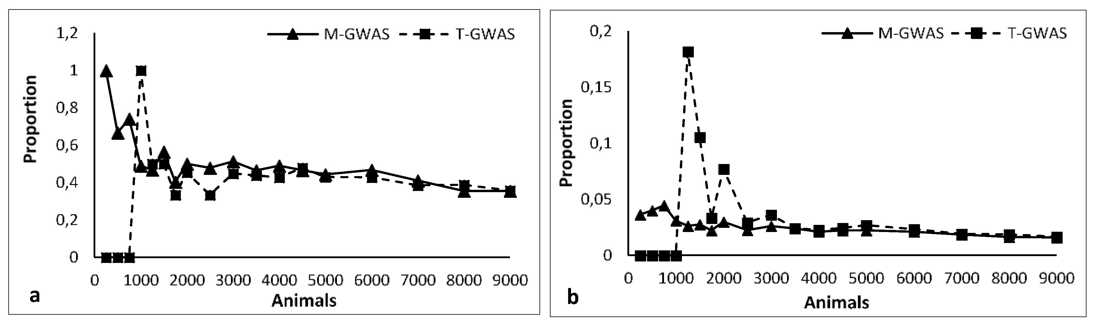
3.1. Simulated Data
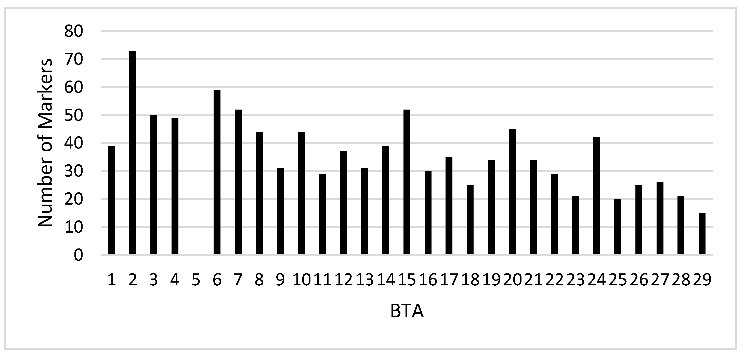
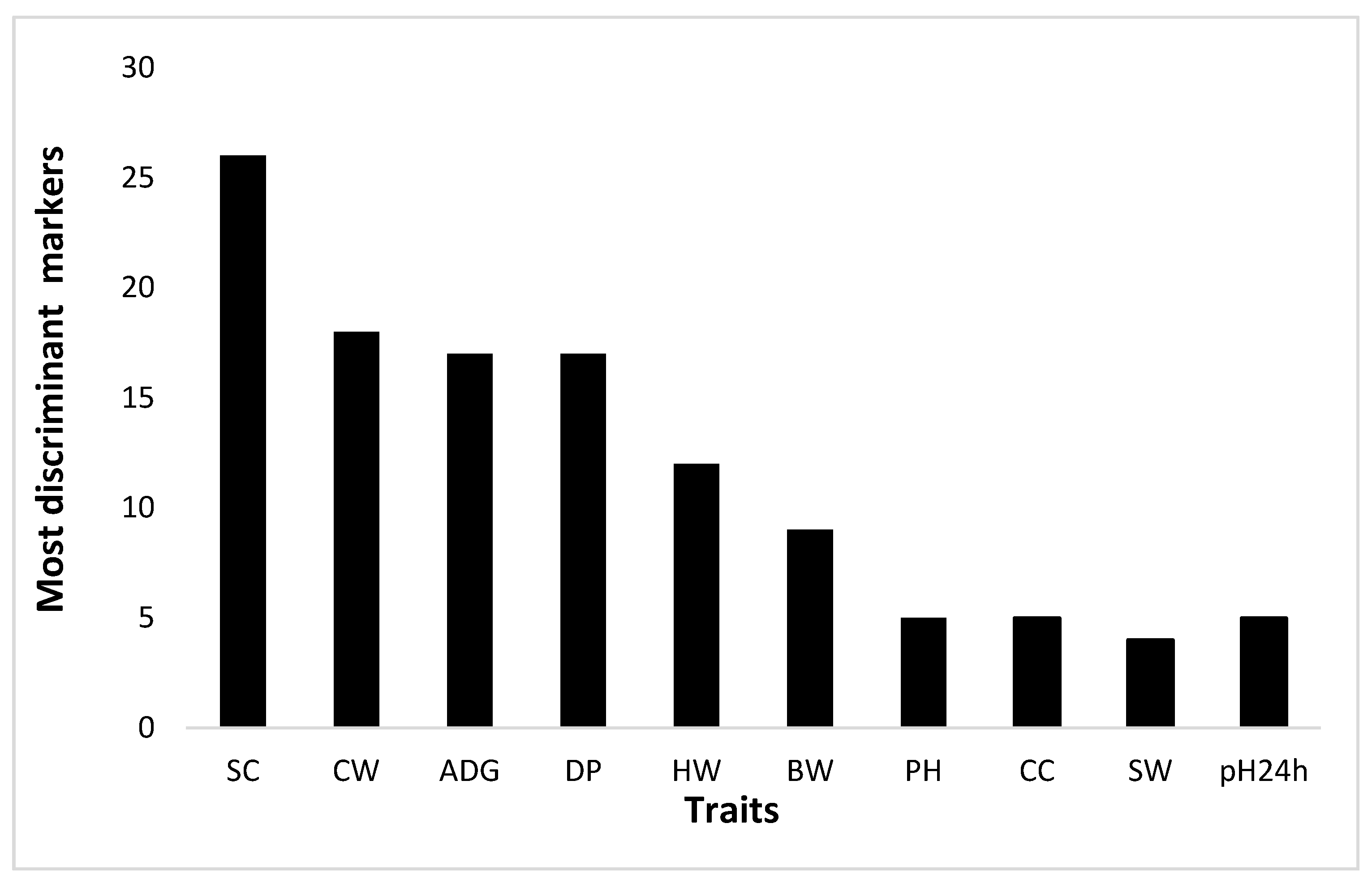
3.2. Real Data
3.3. Gene Discovery
4. Discussion
4.1. Simulation Study
4.2. Real Study
5. Conclusions
Supplementary Materials
Author Contributions
Funding
Conflicts of Interest
References
- Bush, W.S.; Moore, J.H. Genome-wide association studies. PLoS Comput. Biol. 2012, 8, e1002822. [Google Scholar] [CrossRef] [PubMed] [Green Version]
- Benjamini, Y.; Hochberg, J. Controlling the false discovery rate: A practical and powerful approach to multiple testing. J. Roy. Stat. Soc. B Met. 1995, 57, 289–300. [Google Scholar] [CrossRef]
- Bolormaa, S.; Pryce, J.; Hayes, B.J.; Goddard, M.E. Multivariate analysis of a genome-wide association study in dairy cattle. J. Dairy Sci. 2010, 93, 3818–3833. [Google Scholar] [CrossRef] [PubMed] [Green Version]
- Maher, B. Personal genomes: The case of the missing heritability. Nature 2008, 456, 18–21. [Google Scholar] [CrossRef] [PubMed]
- Visscher, P.M.; Yang, J.; Goddard, M.E. A commentary on ‘common SNPs explain a large proportion of the heritability for human height’ by Young et al. (2010). Twin Res. Hum. Genet. 2010, 13, 517–524. [Google Scholar] [CrossRef] [Green Version]
- Meuwissen, T.H.E.; Hayes, B.J.; Goddard, M.E. Prediction of total genetic value using genome-wide dense marker maps. Genetics 2001, 157, 1819–1829. [Google Scholar]
- Erbe, M.; Hayes, B.J.; Matukumalli, L.K.; Goswami, S.; Bowman, P.J.; Reich, C.; Mason, B.; Goddard, M. Improving accuracy of genomic predictions within and between dairy cattle breeds with imputed high-density single nucleotide polymorphism panels. J. Dairy Sci. 2012, 9, 4114–4129. [Google Scholar] [CrossRef] [Green Version]
- Moser, G.; Lee, S.H.; Hayes, B.J.; Goddard, M.E.; Wray, N.R.; Visscher, P.M. Simultaneous discovery, estimation and prediction analysis of complex traits using a bayesian mixture model. PLoS Genet. 2015, 11, e1004969. [Google Scholar] [CrossRef]
- Hayes, B.J.; Pryce, J.; Chamberlain, A.J.; Bowman, P.J.; Goddard, M.E. Genetic architecture of complex traits and accuracy of genomic prediction: Coat colour, milk-fat percentage, and type in Holstein cattle as contrasting model traits. PLoS Genet. 2010, 6, e1001139. [Google Scholar] [CrossRef] [Green Version]
- Dimauro, C.; Cellesi, M.; Steri, R.; Gaspa, G.; Sorbolini, S.; Stella, A.; Macciotta, N.P.P. Use of the canonical discriminant analysis to select SNP markers for bovine breed assignment and traceability purposes. Anim. Genet. 2013, 44, 377–382. [Google Scholar] [CrossRef]
- Dimauro, C.; Nicoloso, L.; Cellesi, M.; Macciotta, N.P.P.; Ciani, E.; Moioli, B.; Pilla, F.; Crepaldi, P. Selection of discriminant SNP markers for breed and geographic assignment of Italian sheep. Small Rumin. Res. 2015, 128, 27–33. [Google Scholar] [CrossRef]
- Figueroa, A.; Caballero-Villalobos, J.; Angón, E.; Arias, R.; Garzón, A.; Perea, J.M. Using multivariate analysis to explore the relationships between color, composition, hygienic quality, and coagulation of milk from Manchega sheep. J. Dairy Sci. 2020, 103, 4951–4957. [Google Scholar] [CrossRef] [PubMed]
- Sorbolini, S.; Gaspa, G.; Steri, R.; Dimauro, C.; Cellesi, M.; Stella, A.; Marras, G.; Ajmone Marsan, P.; Valentini, A.; Macciotta, N.P.P. Use of canonical discriminant analysis to study signatures of selection in cattle. Genet. Sel. Evol. 2016, 48, 58. [Google Scholar] [CrossRef] [PubMed] [Green Version]
- Biffani, S.; Dimauro, C.; Macciotta, N.P.P.; Rossoni, A.; Stella, A.; Biscarini, F. Predicting haplotype carriers from SNP genotypes in bos taurus through linear discriminant analysis. Genet. Sel. Evol. 2015, 47, 4. [Google Scholar] [CrossRef] [PubMed] [Green Version]
- Sorbolini, S.; Bongiorni, S.; Cellesi, M.; Gaspa, G.; Dimauro, C.; Valentini, A.; Macciotta, N.P.P. Genome wide association study on beef production traits in Marchigiana cattle breed. J. Anim. Breed. Genet. 2017, 134, 43–48. [Google Scholar] [CrossRef] [Green Version]
- Sargolzaei, M.; Schenkel, F.S. QMSim: A large-scale ge- nome simulator for livestock. Bioinformatics 2009, 25, 680–681. [Google Scholar] [CrossRef] [Green Version]
- Solberg, T.R.; Sonesson, A.K.; Woolliams, J.A.; Meuwissen, T.H.E. Genomic selection using different marker types and densities. J. Anim. Sci. 2008, 86, 2447–2454. [Google Scholar] [CrossRef] [Green Version]
- Marees, A.T.; De Kluiver, H.; Stringer, S.; Vorspan, F.; Curis, E.; Marie-Claire, C.; Derks, E.M. A tutorial on conducting genome-wide association studies: Quality control and statistical analysis. Int. J. Meth. Psych. Res. 2018, 27, e1608. [Google Scholar] [CrossRef]
- Pasam, R.K.; Bansal, U.; Daetwyler, H.D.D.; Forrest, K.L.; Wong, D.D.; Petkowski, J.; Willey, N.; Randhawa, M.; Chhetri, M.; Miah, H.; et al. Detection and validation of genomic regions associated with resistance to rust diseases in a worldwide hexaploid wheat landrace collection using BayesR and mixed linear model approaches. Theor. Appl. Genet. 2017, 130, 777–793. [Google Scholar] [CrossRef]
- De Maesschalck, R.; Jouan, R.D.; Massart, D.L. The mahalanobis distance. Chemometr. Intell. Lab. 2000, 50, 1–18. [Google Scholar] [CrossRef]
- Dimauro, C.; Cellesi, M.; Pintus, M.A.; Macciotta, N.P.P. The impact of the rank of marker variance–covariance matrix in principal component evaluation for genomic selection applications. J. Anim. Breed. Genet. 2011, 128, 440–445. [Google Scholar] [CrossRef] [PubMed]
- Mardia, K.V.; Kent, J.T.; Bibby, J.M. Multivariate Analysis; Academic Press: London, UK, 2000. [Google Scholar]
- Schmid, M.; Bennewitz, J. Invited review: Genome-wide association analysis for quantitative traits in livestock–a selective review of statistical models and experimental designs. Arch. Anim. Breed. 2017, 60, 335–346. [Google Scholar] [CrossRef]
- Izpisúa, B.J.C.; Duboule, D. Homeobox genes and pattern formation in the vertebrate limb. Dev. Biol. 1992, 152, 26–36. [Google Scholar] [CrossRef]
- Hwang, S.J.; Beaty, T.H.; McIntosh, I.; Hefferon, T.; Panny, S.R. Association between homeobox-containing gene MSX1 and the occurrence of limb deficiency. Am. J. Med. Genet. 1998, 75, 419–423. [Google Scholar] [CrossRef]
- Buss, C.; Petrini, J.; Mourao, G.; Geistlinger, L.; Wolf, J.; Diniz, W.D.S.; Rocha, M.I.P.; Afonso, J.; Oliveira, d.L.A.; Tizioto, P.C.; et al. Identification of a pleiotropic locus for beef quality and feed efficiency in cattle using bi-trait genome-wide association analysis. In Workshop on Omics Strategies Applied to Livestock Science, Proceedings of the Embrapa Pecuária Sudeste-Resumo em Anais de Congresso (ALICE), Piracicaba, Brazil, 24–26 April 2017; Embrapa Pecuária Sudeste: São Carlos, CA, USA, 2017. [Google Scholar]
- Yue, S.J.; Zhao, Y.Q.; Gu, X.R.; Yin, B.; Jiang, Y.L.; Wang, Z.H.; Shi, K.R. A genome wide association study suggests new candidate genes for milk production traits in Chinese Holstein cattle. Anim. Genet. 2017, 48, 677–681. [Google Scholar] [CrossRef] [PubMed]
- Howard, J.T.; Kachman, S.D.; Snelling, W.M.; Pollak, E.J.; Ciobanu, D.C.; Kuehn, L.A.; Spangler, M.L. Beef cattle body temperature during climatic stress: A genome-wide association study. Int. J. Biometeorol. 2014, 58, 1665–1672. [Google Scholar] [CrossRef] [PubMed] [Green Version]
- Sevane, N.; Armstrong, E.; Wiener, P.; Wong, R.P.; Dunner, S. Polymorphisms in twelve candidate genes are associated with growth, muscle lipid profile and meat quality traits in eleven European cattle breeds. Mol. Biol. Rep. 2014, 41, 4721–4731. [Google Scholar] [CrossRef]
- Dunner, S.; Sevane, N.; García, D.; Cortés, O.; Valentini, A.; Williams, J.L.; Mangin, B.; Canón, J.; Levézel, H. Association of genes involved in carcass and meat quality traits in 15 European bovine breeds. Livest. Sci. 2013, 154, 34–44. [Google Scholar] [CrossRef]

| Animals | M-GWAS | T-GWAS | ||||
|---|---|---|---|---|---|---|
| Associated SNP | True Associated SNP | QTL 1 | Associated SNP | True Associated SNP | QTL | |
| 250 | 110 | 4 | 4 | 0 | 0 | 0 |
| 500 | 300 | 18 | 12 | 0 | 0 | 0 |
| 750 | 450 | 27 | 20 | 0 | 0 | 0 |
| 1000 | 650 | 41 | 20 | 2 | 1 | 1 |
| 1250 | 840 | 47 | 22 | 11 | 4 | 2 |
| 1500 | 1130 | 55 | 31 | 38 | 8 | 4 |
| 1750 | 1310 | 72 | 29 | 120 | 12 | 4 |
| 2000 | 1540 | 92 | 46 | 130 | 22 | 10 |
| 2500 | 2000 | 94 | 45 | 240 | 21 | 7 |
| 3000 | 2500 | 127 | 65 | 359 | 29 | 13 |
| 3500 | 3050 | 157 | 73 | 1331 | 73 | 32 |
| 4000 | 3300 | 141 | 69 | 1816 | 96 | 41 |
| 4500 | 3700 | 176 | 82 | 2209 | 113 | 54 |
| 5000 | 4300 | 217 | 96 | 2713 | 170 | 73 |
| 6000 | 5000 | 225 | 105 | 3052 | 166 | 71 |
| 7000 | 5500 | 249 | 102 | 4578 | 226 | 87 |
| 8000 | 7000 | 321 | 114 | 6217 | 299 | 116 |
| 9000 | 7500 | 336 | 119 | 7313 | 339 | 121 |
| Animals | B-GWAS1 | B-GWAS2 | ||||
|---|---|---|---|---|---|---|
| Associated SNP | True Associated SNP | QTL 1 | Associated SNP | True Associated SNP | QTL | |
| 250 | 0 | 0 | 0 | 110 | 2 | 2 |
| 500 | 1 | 0 | 0 | 300 | 15 | 14 |
| 750 | 0 | 0 | 0 | 450 | 30 | 20 |
| 1000 | 2 | 1 | 1 | 650 | 55 | 33 |
| 1250 | 4 | 1 | 1 | 840 | 38 | 27 |
| 1500 | 7 | 1 | 1 | 1130 | 49 | 32 |
| 1750 | 8 | 1 | 1 | 1310 | 54 | 32 |
| 2000 | 14 | 2 | 2 | 1540 | 99 | 58 |
| 2500 | 14 | 3 | 3 | 2000 | 107 | 64 |
| 3000 | 20 | 4 | 3 | 2500 | 119 | 63 |
| 3500 | 21 | 3 | 3 | 3050 | 161 | 81 |
| 4000 | 32 | 4 | 3 | 3300 | 190 | 94 |
| 4500 | 32 | 5 | 5 | 3700 | 185 | 80 |
| 5000 | 41 | 9 | 6 | 4300 | 263 | 115 |
| 6000 | 45 | 8 | 7 | 5000 | 286 | 102 |
| 7000 | 55 | 8 | 7 | 5500 | 305 | 124 |
| 8000 | 57 | 10 | 7 | 7000 | 383 | 144 |
| 9000 | 67 | 8 | 7 | 7500 | 406 | 151 |
| M-GWAS vs. | |||
|---|---|---|---|
| Animals | T-GWAS | B-GWAS1 | B-GWAS2 |
| 250 | – | – | 0 |
| 500 | – | – | 4 |
| 750 | – | – | 5 |
| 1000 | 1 | 1 | 9 |
| 1250 | 1 | 1 | 7 |
| 1500 | 2 | 1 | 13 |
| 1750 | 1 | 1 | 9 |
| 2000 | 5 | 1 | 20 |
| 2500 | 4 | 2 | 20 |
| 3000 | 6 | 2 | 28 |
| 3500 | 17 | 2 | 39 |
| 4000 | 19 | 2 | 41 |
| 4500 | 26 | 4 | 34 |
| 5000 | 42 | 5 | 60 |
| 6000 | 45 | 5 | 58 |
| 7000 | 53 | 6 | 68 |
| 8000 | 67 | 5 | 82 |
| 9000 | 78 | 5 | 90 |
| Trait | T-GWAS SNP | M-GWAS SNP | M-GWAS v.s T-GWAS SNP | Minimum Number of M-GWAS SNP |
|---|---|---|---|---|
| BW 1 | 5 | 191 | 4 | 94 |
| ADG 2 | 45 | 193 | 30 | 139 |
| CW 3 | 9 | 191 | 4 | 98 |
| DP 4 | 12 | 191 | 10 | 98 |
| SC 5 | 13 | 193 | 6 | 108 |
| HW 6 | 7 | 192 | 5 | 99 |
| pH 7 | 5 | 190 | 1 | 120 |
© 2020 by the authors. Licensee MDPI, Basel, Switzerland. This article is an open access article distributed under the terms and conditions of the Creative Commons Attribution (CC BY) license (http://creativecommons.org/licenses/by/4.0/).
Share and Cite
Manca, E.; Cesarani, A.; Gaspa, G.; Sorbolini, S.; Macciotta, N.P.P.; Dimauro, C. Use of the Multivariate Discriminant Analysis for Genome-Wide Association Studies in Cattle. Animals 2020, 10, 1300. https://doi.org/10.3390/ani10081300
Manca E, Cesarani A, Gaspa G, Sorbolini S, Macciotta NPP, Dimauro C. Use of the Multivariate Discriminant Analysis for Genome-Wide Association Studies in Cattle. Animals. 2020; 10(8):1300. https://doi.org/10.3390/ani10081300
Chicago/Turabian StyleManca, Elisabetta, Alberto Cesarani, Giustino Gaspa, Silvia Sorbolini, Nicolò P.P. Macciotta, and Corrado Dimauro. 2020. "Use of the Multivariate Discriminant Analysis for Genome-Wide Association Studies in Cattle" Animals 10, no. 8: 1300. https://doi.org/10.3390/ani10081300