This section introduces the definition of small targets and the network model used to perform small-target detection.
2.1. Small Target Definition
The definitions of small targets are divided into two categories according to the scale and size of the target objects: relative definition and absolute definition. Relative definition means that the size of the target is smaller than a certain percentage of the original dataset image; for example, the small-target objects in the Stanford Drone dataset [
14] are smaller than 0.2% of the original image size and the median value of the relative area (the ratio of the area of the bounding box to the area of the image) of the defined small target in the PASCAL-VOC dataset [
15] is less than 5%. The absolute definition specifies that the pixels of the target must be less than a certain value to be defined as a small target, such as the AI-TOD [
16] dataset, which defines 8–16 pixels as a tiny target and 16–32 pixels as a small target; the DIOR [
17] dataset defines the width or height of a small target as less than 50 pixels.
Based on specific applications and research scenarios, different definitions of small targets have been given by researchers for specific datasets. Referring to the face detection dataset WIDER FACE [
18], which defines the scale of small targets for faces as 10–50 pixels, and the daily items SDOD-MT [
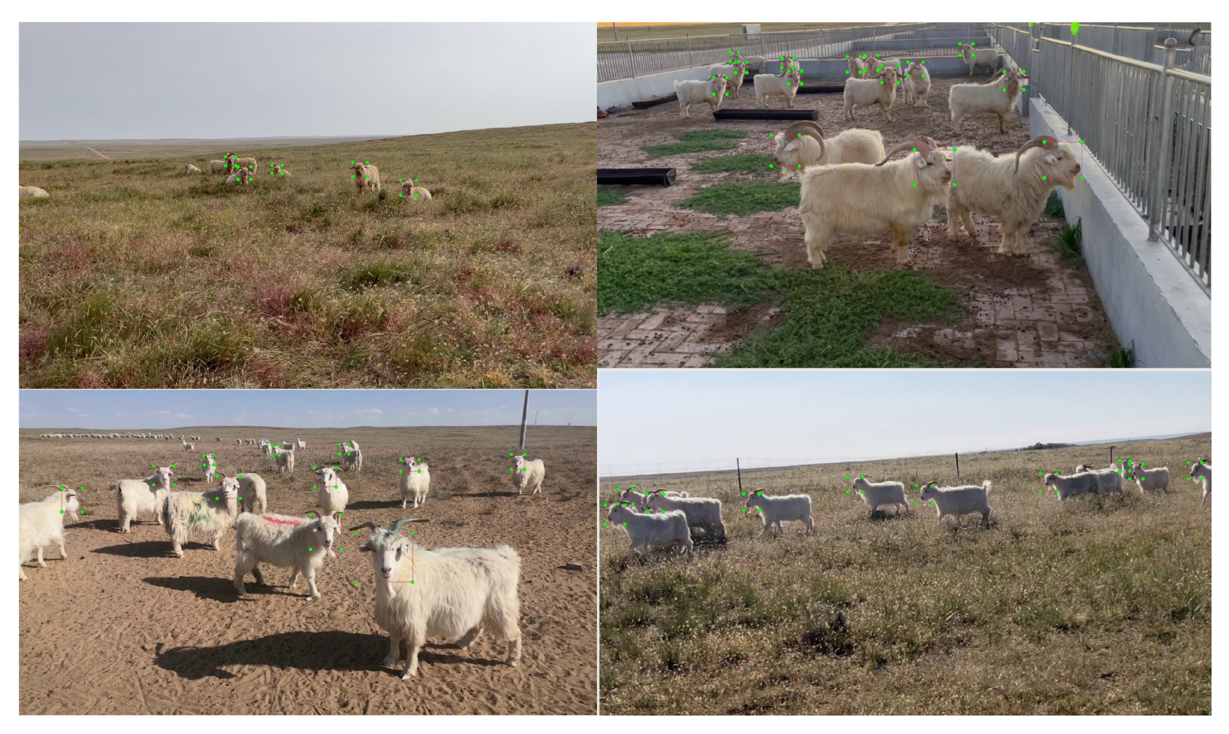
19] dataset, which similarly defines the range of small targets as 10–50 pixels depending on the length of the horizontal bounding box, we specified that targets must be smaller than 50 pixels in the goat face dataset to be classified as small-target goat faces.
2.3. Context Information Detection Module
The detection of small goat face targets presents a formidable challenge due to multiple factors. Notably, acquired goat face targets exhibit blurriness, inconspicuous features, and considerable environmental interference. Furthermore, these small goat face targets typically occupy only a few pixels within the overall image, further exacerbating their susceptibility to noise, texture, and other disruptive factors. Consequently, accurately identifying and locating these small targets becomes arduous. To address the issue of substantial interference and the resulting low detection accuracy in goat face small target detection, we proposed a contextual information detection module. This module leverages the contextual information surrounding the target, enabling the acquisition of additional background information and contextual semantic cues. By incorporating such contextual information, the proposed module offers tangible benefits for the detection and localization of small targets.
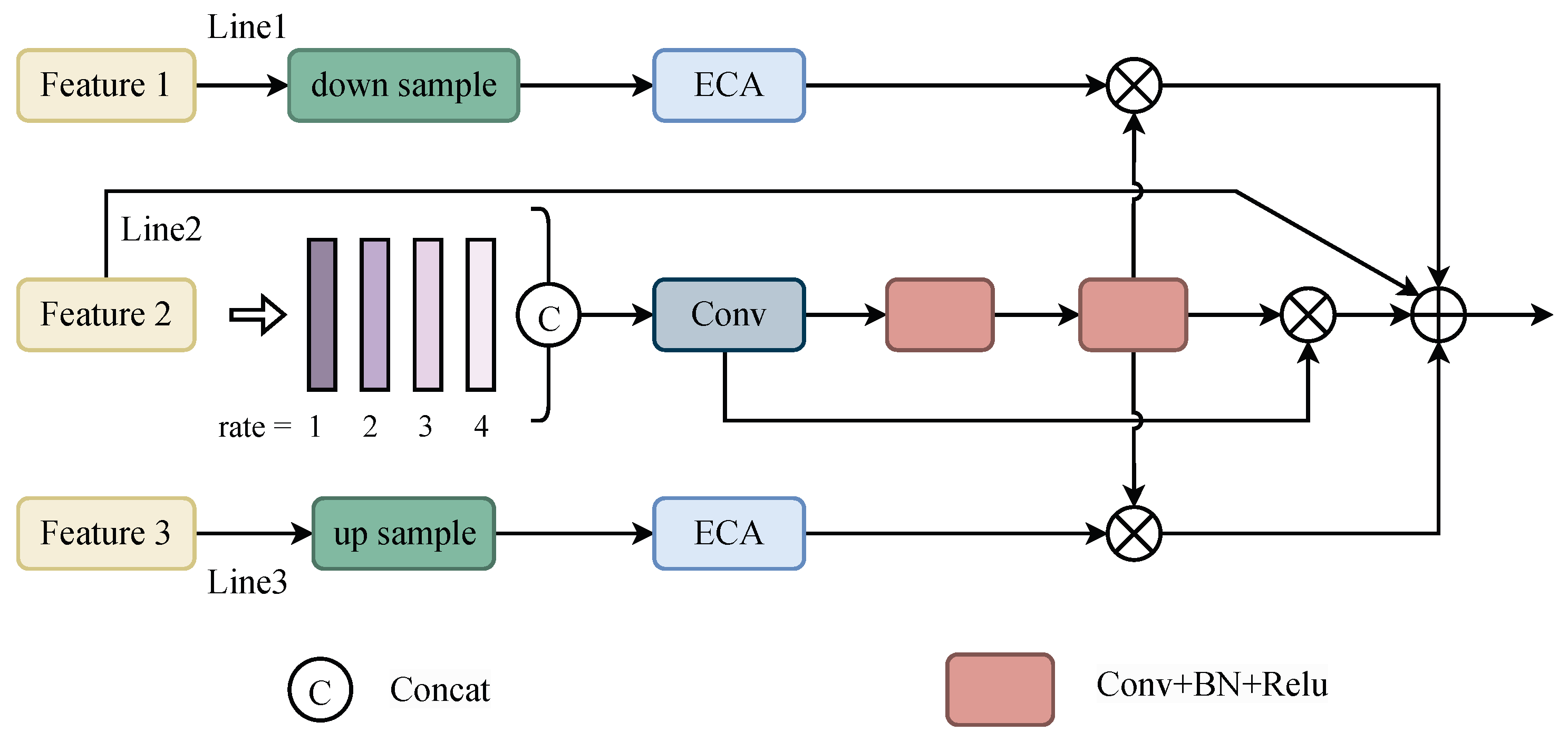
We used a dilated convolution with different convolution rate sizes to form different receptive fields and extract local contextual information. As shown in the local context extraction backbone in
Figure 2, a multi-branch convolutional block exists, in which each branch will extract information from different perceptual fields. We used dilated convolution with convolutional rates of 1, 2, 3, and 4 to extract information; to extract more information, the convolutional kernel size was increased to
, and the extracted information was fused by a cat operation to form local contextual information.
where
is concatenation and
is the dilated convolution with different convolution rates.
Local contextual information often exists in a feature layer. In order to obtain global contextual information in the surrounding environment, it is necessary to combine feature information from adjacent feature layers; therefore, we introduced feature interactions between features at adjacent levels and, since the previous and subsequent features have different scales to the current feature, the two adjacent branches were, respectively, upsampled and downsampled after convolution to align the number of channels. Then, the extraneous information generated in the feature interactions was suppressed by the ECA attention module [
23] to reduce the sensitivity to noise and interference.
where
and
are upsampling and downsampling operations, respectively, and
is the ECA attention mechanism, an efficient attention module.
2.4. Feature Complementary Module
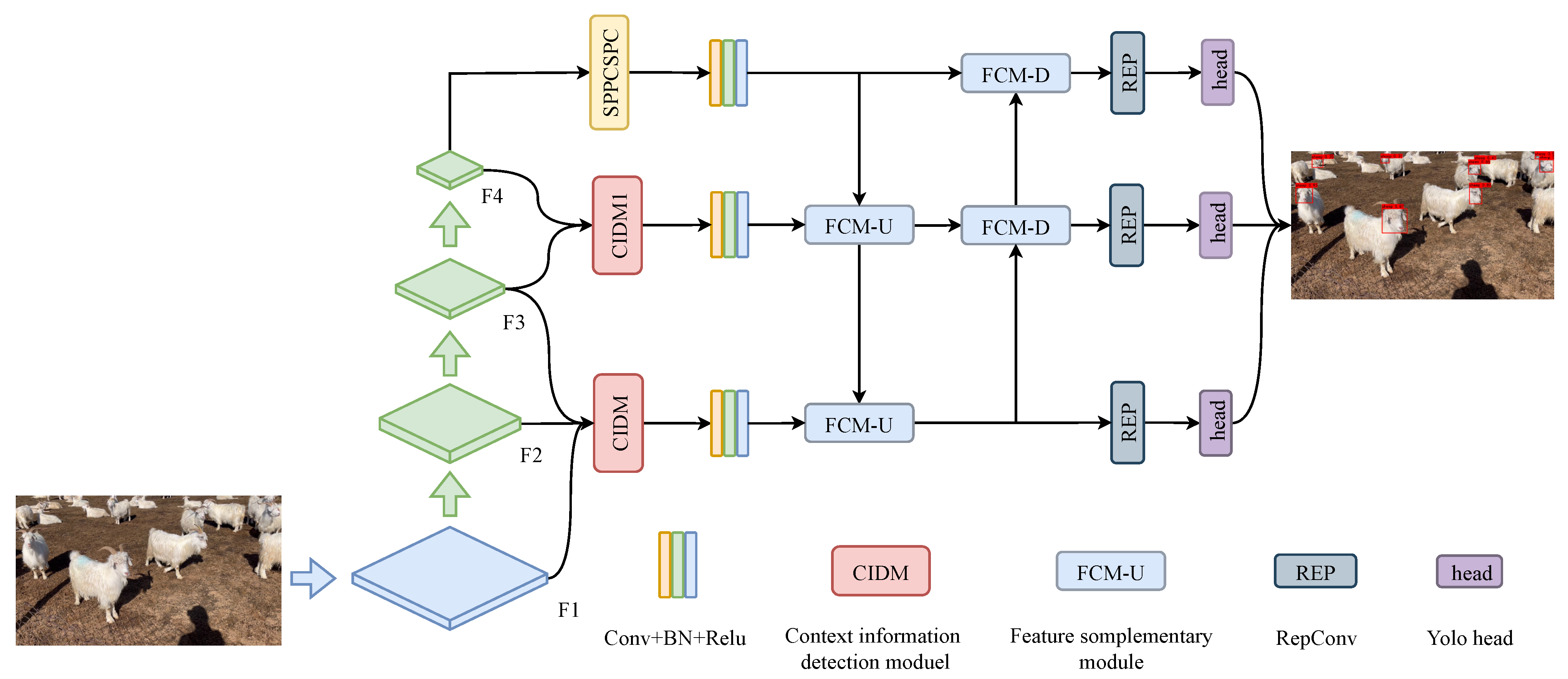
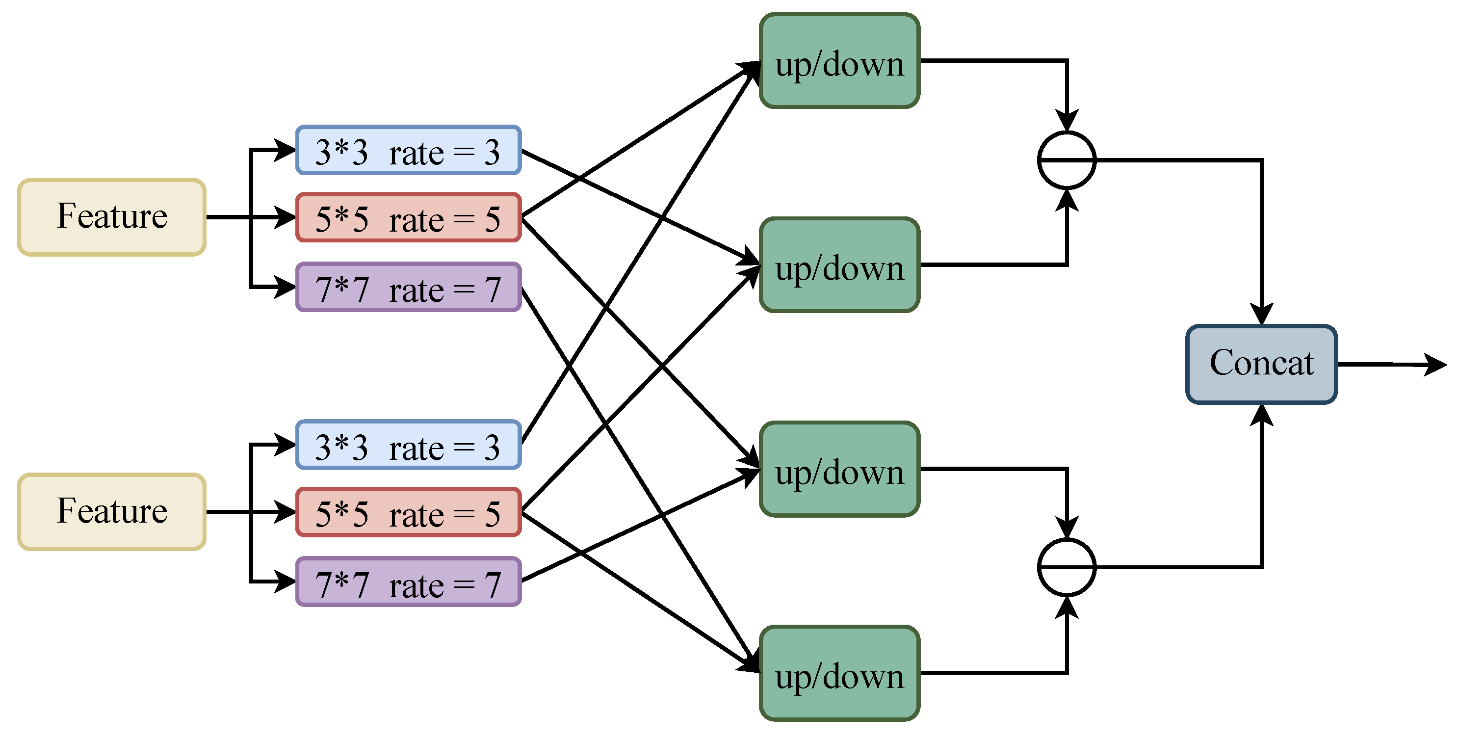
To fuse the feature maps generated at the different stages, we proposed FCM-U and FCM-D, as shown in
Figure 3. FCM-U aggregates the three features generated by the contextual information detection module and SPPCSPC and aligns the number of channels to improve the feature resolution and generate a new feature map in FCM-D to fuse the features generated in the previous stage. In FCM-U and FCM-D, we used convolution kernels of 3, 5, and 7 for dilation convolution to receive the correct number of channels for feature alignment, and then divided these two by two into UP or DOWN modules to improve and reduce the feature resolution. Finally, a differencing operation was performed to fuse the features and suppress the background noise generated during feature-fusion by differencing.
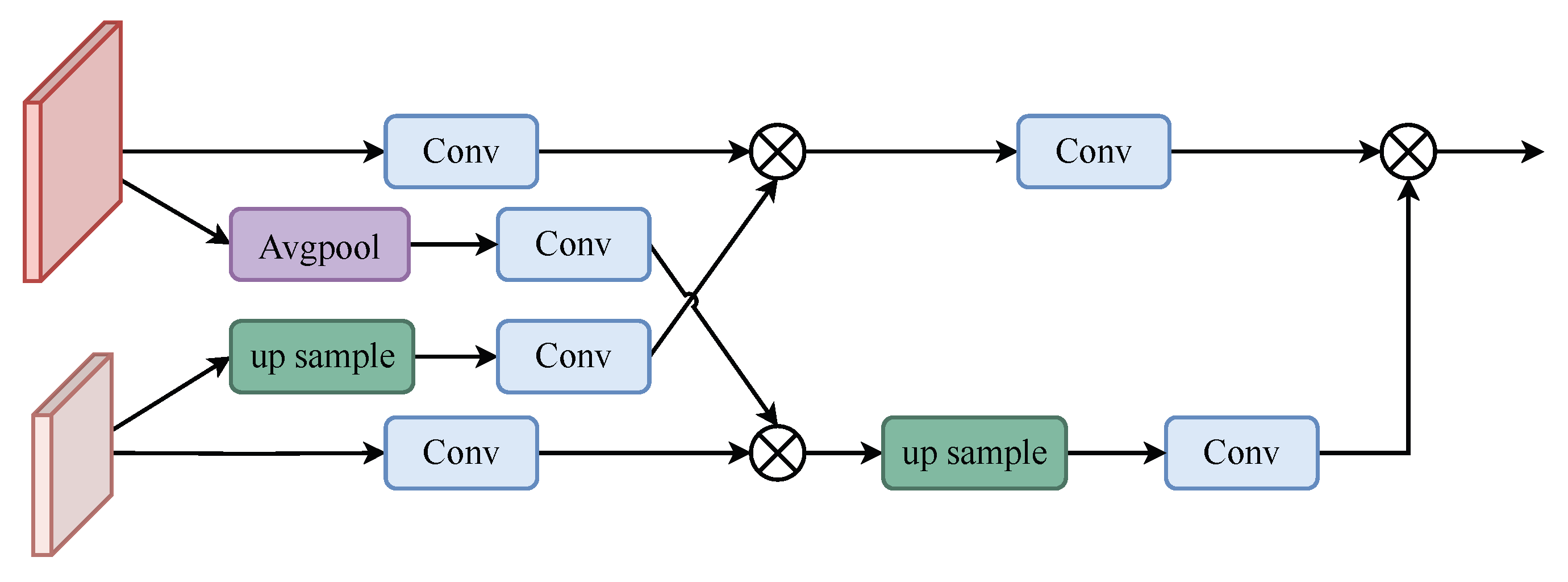
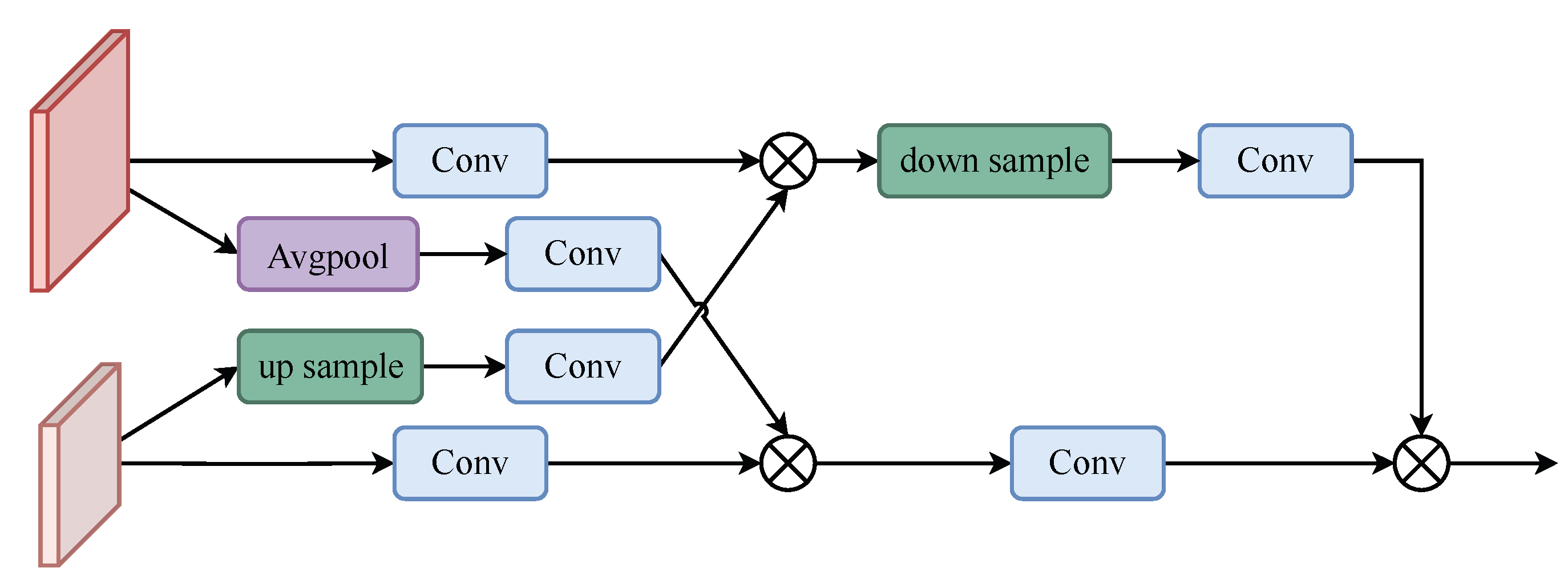
As shown in
Figure 4, the high-resolution feature
is downsampled by averaging pooling to obtain
, and the low-resolution feature
is upsampled by bilinear interpolation to obtain
.
and
are then convolved
to obtain
and
, respectively. The convolved
is multiplied by
to obtain the feature
.
Similarly, multiply the convolved
with
to obtain the feature
.
Finally, the upsampled
is
passed through the convolution block and multiplied with the convolved
,
to obtain the output feature. The operation can be expressed as follows:
The down module is similar to the up module;as shown in
Figure 5 the only difference is that, instead of upsampling
,
is downsampled
through the convolution block and multiplied through the convolution block with
to obtain the output features. The operation is given in the following equation:
After
or
, the output features are set after the differential module to output the final feature results. The differential module can effectively offset noise and interference, thus improving the reliability and anti-interference ability of the feature target. The equation is as follows:
,
are the output of the previous stage and
is the absolute value operation.
and
are the outputs of difference in
Figure 3, respectively, while
is a concatenation operation.
2.5. Small-Target Detection Head and Loss Function
The anchor frame sizes of YOLOV7 were set to 12, 16, 19, 36, 40, 28, 36, 75, 76, 55, 72, 146, 142, 110, 192, 243, 459, and 401, which are very scientific for target detection but not suitable for our small-target goat face detection. In order to set the anchor frame at an appropriate size, we first performed a cluster analysis on the training set anchor frame size using the clustering algorithm. The maximum target to be detected was revealed to be 55 and the minimum was 8. Most of the edge labels of the target to be detected were concentrated from 24 to 32; therefore, we set the anchor frame sizes as 5, 9, 12, 16, 19, 36, 42, 31, 40, 28, 55, 48, 36, 75, 76, 55, 72, and 146 to improve the detection accuracy for small targets.
The values of the loss function of YOLOV7 include target confidence loss, category confidence loss, and coordinate regression loss.
Binary cross entropy is a common loss function used here to calculate confidence loss and category loss.
The localization loss
can be calculated using
[
24],
[
25],
[
26], and
[
27] for loss calculation. IoU is the most commonly used metric in target detection, and can be used to evaluate the distance between the prediction frame and the ground true. The
formula is as follows:
differs from
in that it can focus on non-overlapping regions, and the
formula is as follows:
can focus on the distance, overlap and scale of the target and anchor; the equation of
is as follows:
is the addition of the detection box scale loss to
;
is as follows:
where
represents the ground-truth value,
represents the prediction frame, and
represents the area of the smallest closure region that contains both the prediction frame and the ground truth frame,
represents the centroid of the predicted frame,
represents the centroid of the ground truth frame,
is the Euclidean distance between the centroids of the truth frame and the predicted frame, d represents the minimum value of the diagonal of the region containing both the predicted frame and the ground truth frame,
is the weight function, and
v is the parameter used to measure the consistency of the aspect ratio, which is given by the following equation:
where
represents the aspect ratio of the ground truth frame and
represents the aspect ratio of the predicted frame.
takes into account the difference in the bounding box width-to-height ratio instead of the difference between the predicted box and the ground truth box width and height truth, which can hinder the model regression in some cases. When
=
: when the predicted box width–height ratio is equal to the ground true box width–height ratio, the value of the
v term of
is 0, which means that its penalty term will be useless and will degrade to
. Based on the above, our
was based on the proposed
, the width–height ratio was split and the variance in width and height relative to their true values were calculated separately, which can directly obtain the minimum value of the difference, which is more conducive to model convergence, and the
formula is as follows:
is the ratio of the width of the prediction box to the width of the ground true box,
is the ratio of the height of the prediction box to the height of the ground true box.
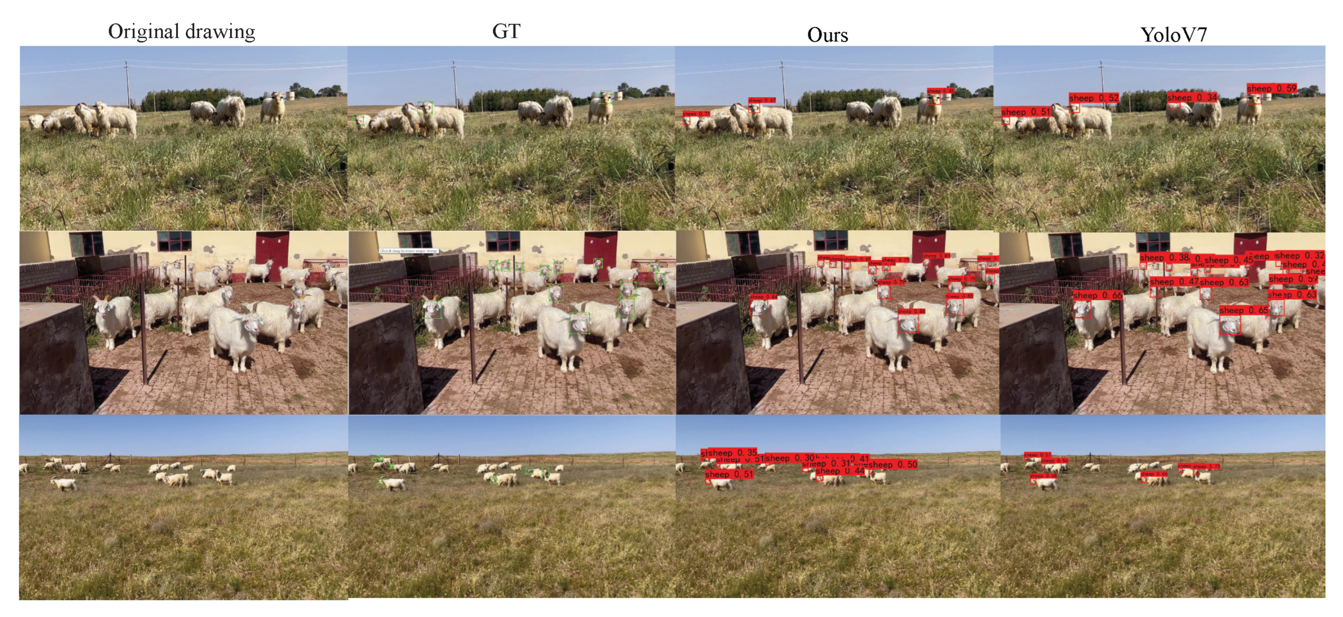
The individual IoUs were compared in the
Section 3.


