1. Introduction
Animals whose survival depends on early target detection are often equipped with a sharply tuned visual system, yielding robust performance in challenging conditions. Complex scene perception depends upon the interaction between signals from the classical receptive field (CRF) and the extra-classical receptive field (eCRF) in visual neurons [
1]. Among them, there is a fundamental neural phenomenon known as “surround suppression”. This phenomenon has been widely reported to exist in many levels of the visual system, including the retina [
2,
3], superior colliculus (SC) [
4], lateral geniculate nucleus (LGN) [
5], and primary visual cortex (V1) [
6,
7], in mammals and the optic tectum (OT) [
8,
9,
10] in non-mammals. This fundamental neuronal property is associated with visual saliency representation, allowing efficient information encoding. The electrophysiological experiments further show that the suppression degree could be modulated by stimuli contrast between the center and surroundings [
11,
12,
13]. The suppression is strongest in homogeneous visual contexts, where the surrounding stimuli are similar to those in the center [
14]. Recent work has reported that the suppression engendered by motion direction contrasting stimuli was stronger than that by static luminance contrasting stimuli [
12], suggesting that encoding strategies of luminance and motion contrasting stimuli may be different. Furthermore, under the motion mode, the surround modulation index induced by luminance contrast is lower than that under the static mode (authors, unpublished data), suggesting that the surround modulation pattern of OT neurons is dynamic, not only related to the degree of contrast between the center and surroundings but also associated with the state of the target (stimulus mode). However, it is still unclear how they differ and where the difference was derived from. The answer would help with further understanding the underlying encoding mechanisms of surround suppression, which plays an important role in enhancing contrast sensitivity and effectively reducing redundant information in the visual environment.
Abundant existing studies imply that the neuronal processing of external visual information is always nonlinear and the tuning of excitatory and inhibitory inputs might also differ substantially [
15,
16]. However, nonlinear processing was always approximated with a linear module in encoding models [
17,
18] to reduce the modeling complexity and facilitate computational efficiency. Typically, the center–surround effect has been widely explained using a difference of Gaussian (DoG) model [
2,
19], which was defined by the difference of two Gaussian distributions with a narrower positive Gaussian and a broader negative Gaussian. This model assumes that the surround interaction is linear with the fully formed center signal. Furthermore, the generalized linear model (GLM) was always used to link the functional descriptions of visual processing with neural activity recorded across the visual system [
20,
21] and described the encoding process in terms of a series of stages: linear filtering, nonlinear transformation, and Poisson spiking process. Except, GLM was used to characterize neural encoding in a variety of other sensory, cognitive, and motor brain areas [
17,
21]. These existing models also hypothesized that the interaction between excitatory and inhibitory inputs was linear, whereas nonlinearity serves as a typical characteristic that drives the underlying circuitry and promotes sensory integration. It is unclear whether the linear modules instead of nonlinear modules can realistically simulate the encoding process of optic tectal neurons for moving objects.
Meanwhile, it could be implied that center–surround suppression is closely related to the suppression inputs that neurons receive, including those from feedforward, horizontal, and feedback connections [
22]. Recent work also suggested that inhibitions performed on tectal neurons appeared to be fully surrounding rather than locally lateral [
10]. Additionally, a saliency map in the avian optic tectum (OT) is created by the interaction between the OT and the nucleus isthmi. The latter is divided into two streams: the nucleus isthmi pars magnocellularis (Imc) and the nucleus isthmi pars parvocellularis (Ipc) [
23], transmitting inhibitory and excitatory inputs into OT, respectively. Both reductions in excitatory synaptic input and an increase in inhibitory synaptic input lead to a decrease in total synaptic input, which could generate diverse modulation for different contrasting stimuli. However, there is a lack of evidence proving which of these inputs contributed to the diverse contextual modulated responses. Furthermore, it is pretty difficult to accurately describe the encoding process of a complex neuronal network, especially containing such nonlinearity and complex interactions. Fortunately, the conductance-based encoding model (CBEM), as an extension of GLM, could simulate synaptic conductance changes that drive them by not only allowing for differential tunings of excitation and inhibition but also adding rectifying nonlinearities governing the relationship between the stimulus and synaptic input [
24]. The inhibitory and excitatory components could be flexibly adjusted in CBEM. Thus, it is well suited to study the encoding strategies on spatial contrasting stimuli.
Taken together, we hypothesized that diverse surround modulation properties could be regulated by dynamical nonlinear spatial integration between excitation and inhibitory synaptic inputs. Then, the CBEM framework was adopted to establish a contrasting encoding model (Generalized Linear-Dynamic Modulation, GL_DM) to describe the process of encoding contrasting stimuli in tectal neurons, and the parameters were fitted by neuronal data recorded from pigeon OT in the same stimulus paradigms with our previous work [
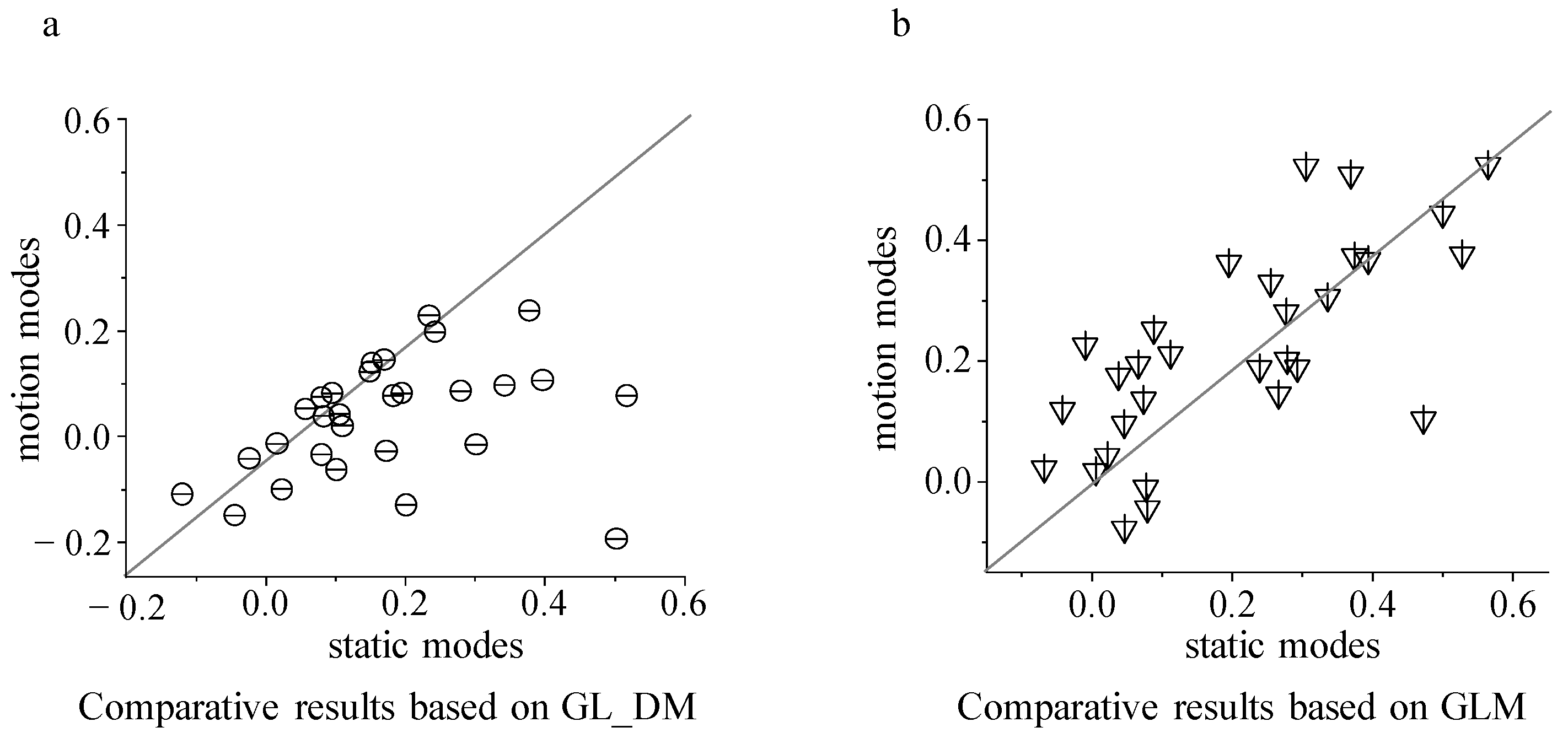
12], including motion direction contrasting stimuli and luminance contrasting stimuli. The results show that the encoding accuracy was improved by taking the nonlinear functions into account, suggesting that the dynamic nonlinear spatial integrations may play an important role in encoding contrasting visual stimuli. Finally, we compared the predicted response by the full-GL_DM and GL_DM with only excitatory synaptic input to verify the factor that affects the modulation difference between luminance and motion contrasting stimuli.
2. Materials and Methods
2.1. The Control Model: The Generalized Linear Model Combined with the Difference of Gaussian Model
The generalized linear model combined with the difference of Gaussian model serves as a control linear model. The model schematic is shown in
Figure 1. It mainly consists of two parts: the difference of Gaussian model and the generalized linear model. The former provides a mapping from stimuli to spike trains, and the latter describes the realistic center–surround receptive field (RF) structure.
The difference of Gaussian model represents the RF center–surround integration and consists of a positive narrow Gaussian function, used to describe the excitability of the receptive field center, and a negative broad Gaussian function to describe the inhibitory ingredients of antagonistic receptive field surroundings. The summation of them represents their mutual antagonism in space. The output is represented by the two Gaussian functions on the spatial domain after linear weighted integral. The function of the DoG filter is expressed as follows:
where
is a Gaussian function with the mean value
, and
and
indicate the size of excitatory RF and inhibitory surrounding RF, respectively.
and
denote the relative strength of excitability and inhibition, respectively.
represents the weaker RF surround strength relative to the RF center.
represents the spatial integrated output between the center and the surroundings.
The generalized linear model is a cascade model, containing linear integration, the nonlinear transition of spike rate, and probabilistic spiking stages of the Poisson process. Spatiotemporal integration of visual inputs from cones is modeled as linear, in which spatial integration is a two-dimensional Gaussian function and temporal integration is a biphasic impulse-response function. The linear integration stage consists of spatiotemporal integration of visual inputs and post-spike filter, in which the former spatial integration of stimulus is described with the DoG model, and temporal integration of stimulus is characterized for a filter
in GLM. The neuron’s membrane potential is defined as follows:
where
is the spatially integrated stimulus (vectorized).
is the stimulus temporal filter.
is the post-spike filter to capture dependencies on spike history.
is a vector representing spike history at time
t.
is a baseline to determine the baseline firing rate in the absence of input.
Then, membrane potential passes through a nonlinear function
to produce the spike rate
as the conditional intensity of a Poisson process.
Finally, the spike trains are obtained by an inhomogeneous Poisson spiking process.
2.2. Contrasting Encoding Model: Generalized Linear-Dynamic Modulation
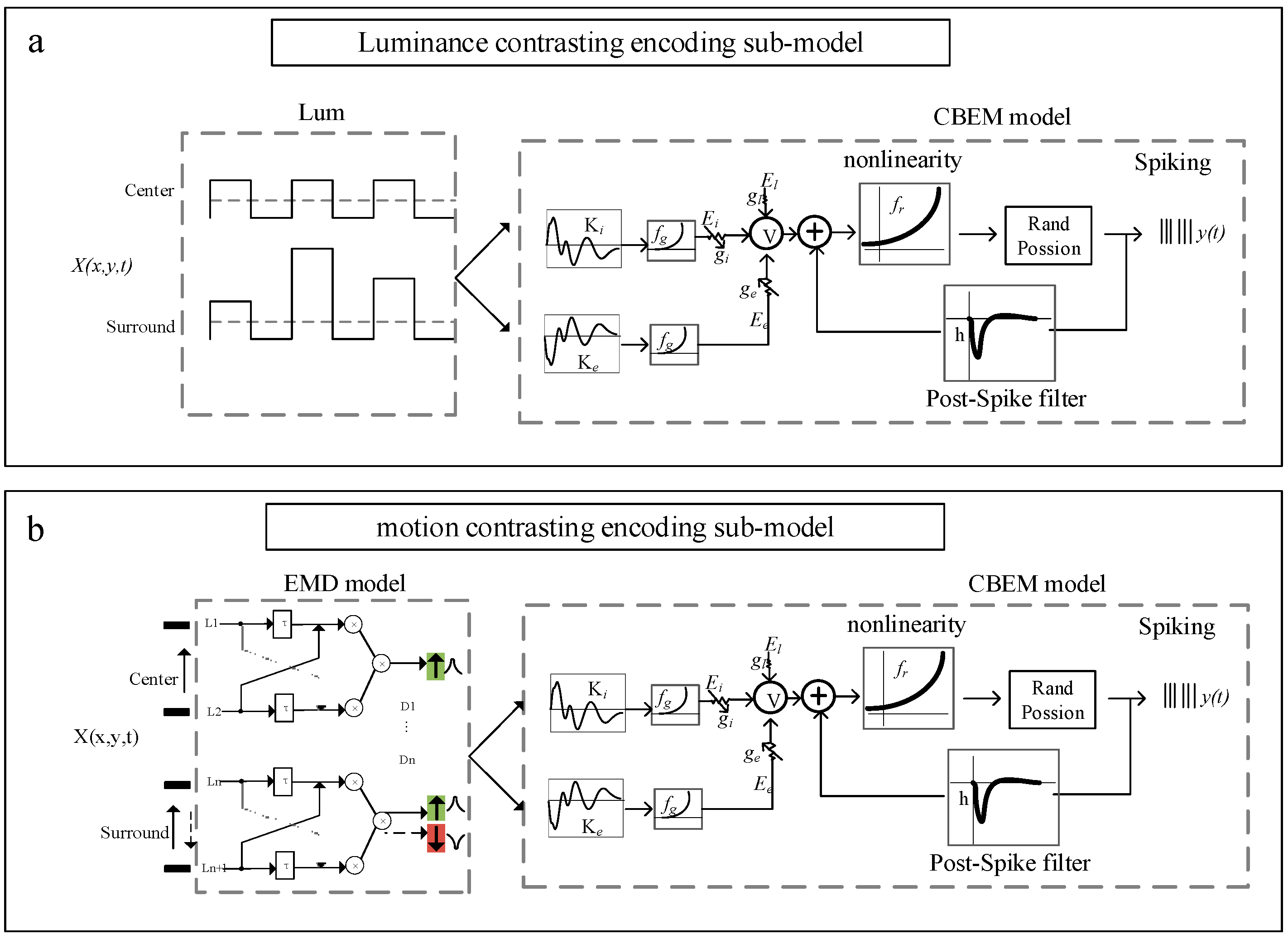
A contrasting encoding model (referred to as GL_DM) is established based on the CBEM framework cascading with a photoelectric transduction model to describe the primary process of encoding contrasting stimuli. In contrast to the GLM, CBEM adds a nonlinear governing relationship between the stimulus and synaptic conductance with independent tunings of excitatory and inhibitory synaptic inputs. GL_DM mainly consists of two parts: the photoelectric transduction model and the CBEM. The former is used to simulate the preprocessing of temporal and spatial stimuli by the retina and tectum, and the latter is used to generate spike trains of OT neurons to specific stimuli. The GL_DM schematic for predicting spike trains of tectal neurons for contrasting stimuli is shown in
Figure 2.
The GL_DM was established to validate encoding strategies by exploring key factors that contribute to the visual response differences between two different types of stimuli (spatial luminance contrasting versus motion direction contrasting). Thus, the inputs of the model contain two different types of visual stimuli (static and moving stimuli), which are processed by two types of photoelectric transduction modules, respectively. As is shown in the green region in
Figure 2a, the static visual stimulus is transduced to electrical activity by normalization of luminance values. At time
, the electrical activity with a range of [−1 1] at a single point in space is defined as follows:
where
is the luminance value at a single point in space.
is the mean luminance value.
and
indicate the maximum and minimum luminance values, respectively.
In contrast to static stimulus, the electrical activity in each spatial pixel is time-varying for moving stimulus (
Figure 2b). The direction of motion stimuli is detected by the full Hassenstein–Reichardt detector (full-HR detector), which consists of two subunits, arranged in a mirror-symmetric fashion and subtracted from each other to yield a fully opponent detector. The output
is defined as follows:
where
and
are two adjacent dendrites to detect the contrast signals from two spatial locations.
denotes the temporal delay.
As a result, the sign of the output is positive for the preferred direction, and negative when motion is along the opposite direction. The preferred direction was defined as the motion direction of the stimulus inside RF since the neurons in this study had no motion direction selectivity [
12].
By using the photoelectric transduction model, the stimulus is transduced as a matrix, serving as the input of CBEM, which is an extension of GLM by adding two linear–nonlinear functions of input to obtain excitatory and inhibitory synaptic conductance, respectively.
Here, is the output of the photoelectric transduction model. and denote the linear excitatory and inhibitory “conductance” filter. The nonlinear function is assumed a “soft-rectification” to ensure that conductance is non-negative. and determine the baseline excitatory and inhibitory conductance in the resting state.
After giving excitatory and inhibitory synaptic conductance, the membrane potential
is defined by an ordinary differential equation:
where
is leak conductance.
,
, and
are the leak, excitatory, and inhibitory reversal potentials.
Then, the spike-history effect is incorporated by adding a linear autoregressive term:
where
is a vector of binned spike history at time
t.
h is the spike-history filter.
Finally, the outputs
pass through a nonlinear function
to obtain the spike rate for an inhomogeneous Poisson spiking process.
The model parameters needing to fit include
,
,
,
and
, all of which are selected using conjugate-gradient methods to maximize the log likelihood. The reversal potential and leak conductance parameters [
25,
26] are kept fixed at
,
,
, and
.
2.3. Electrophysiological Data
The electrophysiological data were selected from the previous work [
12] and recorded from 10 pigeons (Columba livia, homing pigeon, either sex, weighing 300–400 g). The neuronal data were obtained with a polyimide-insulated platinum/iridium micro-electrode array that was arranged in four rows with four wires in each row. The array was lowered about 800 μm–1200 μm below the tectum surface using a micromanipulator.
Two types of center–surround stimulus paradigms were used in this study: one involving luminance stimuli and the other involving motion stimuli. In the luminance contrasting paradigm, a vertical or horizontal bar is placed at the center of the receptive field (RF). Surrounding bars of equal size are positioned parallel to the orientation of the central bar. The luminance of the center bar was set at 0.1 cd/m2. The luminance of the surrounding bars was uniformly set at 0.1 cd/m², 35.1 cd/m², and 70.1 cd/m². In the motion contrasting paradigm, the motion direction and luminance of the center bar were kept the same too. The surrounding bars moved in the same or opposite direction. The luminance of the surrounding bars was uniformly set at 0.1 cd/m² or 70.1 cd/m².
A total of 30 neurons were recorded, with 20 trials collected for each neuron. Fifteen neurons were used for the luminance stimulus paradigm, and nineteen neurons were used for the motion stimulus paradigm. Four neurons were used for both paradigms, resulting in a total of 680 data points.
Each set of parameters was fitted with neuronal responses to two types of center–surround stimuli, including flashed spatial luminance contrasting mode and motion direction contrasting mode with uniform luminance, in which the center bar was at RF center while the surrounding ones varied in luminance and motion direction were distributed outside the RF.
2.4. Evaluation of Model Performance
Firstly, we fit the model parameters to a dataset consisting of two types of center–surround stimuli and their corresponding firing spike trains, and then we used the trained model to predict the spike responses elicited in response to novel stimuli recorded in the same unit. The training set is divided using the 80:20 rule, where 80% of the recordings of each class separately are used for training, and the remaining are used for validation. The model performance was evaluated with the residual error (
) and goodness of fit (
) between the predicted peri-stimulus time histogram (PSTH) and the recorded neuronal response. The PSTH was calculated by averaging spike numbers in 20 ms time bins with smoothing with a Gaussian filter. The residual error is defined as follows:
According to the nature of the residual, ideally the residual points of the model should be evenly distributed on the upper and lower sides of the
straight line. The smaller the residual value, the higher the prediction accuracy of the model. The good-ness fit is defined as follows:
where
and
denote the average value of the PSTH. The value of the rho ranges from −1 to +1, where ±1 indicates a total positive or negative correlation and 0 indicates no correlation.
We also calculated a modulation index to verify whether the proposed model captured their observed surrounding modulation in experimental data. The modulation index is defined as follows: modulation index = (Roddball − Runiform)/(Roddball + Runiform), where Roddball is the response to the center stimulus when it is different from the background elements, and Runiform is the response to the same center stimulus when it is identical to the background elements.
All statistical tests performed in this manuscript were non-parametric Wilcoxon signed-rank tests, unless otherwise stated. Data analysis was performed using MATLAB R2019b (The Mathworks). Graphs and figures were performed using Origin 2019b (Origin Lab, Northampton, CA, USA).
4. Discussion
In this study, we derived a contrasting encoding model for tectal neurons using multi-unit recording data. Data were used to fit model parameters and evaluate different strategies of the tectal neuron encoding luminance and motion contrasting stimuli. The results show that the predicted response is more accurate when using GL_DM with a nonlinear function than GLMD with a linear one, verifying the nonlinearity of integration between excitatory and inhibitory inputs to encoding contrasting stimuli. Furthermore, compared to GL_DM, the GL_DMexc exhibited far larger reductions in prediction response to motion direction contrasting stimuli than that to luminance contrasting stimuli. In summary, these results indicated that tectal neurons may adopt different strategies for encoding luminance and motion contrasting stimuli, and the encoding strategies are closely associated with nonlinear integration and inhibitory synaptic input. This provides some explanation as to how and why neuronal responses to motion contrasting and luminance contrasting stimuli differ, providing new insights for understanding the encoding mechanisms of contrasting stimuli based on center–surround suppression in the visual system.
Nonlinear integration mechanisms have been widely found in mammals [
27]. Previous studies have demonstrated that the nonlinear relationship between excitatory activation and spike response could be changed by the activation of suppressive subunits [
28]. This nonlinear relationship of subunits in the RF center is important for capturing responses to spatially structured stimuli [
29]. In addition, theoretical studies have proved the necessity of nonlinearity, such as rectification, followed by a summation of the preprocessed signal [
30]. In our study, we found that GL_DM with nonlinear integration maintained more accurate predictive performance than the GLM
D, which has only one stimulus filter in which synaptic excitation and inhibition are linearly governed by equal filters of opposite signs. However, the GL_DM’s greater accuracy in predicting neuronal responses is attributable to the flexibility conferred by the slight differences in these filters with separate nonlinearities. The results were in agreement with those found in mammals [
30,
31]. Indeed, the center–surround arrangement of receptive fields is ideal for detecting local contrast changes, and nonlinear spatial integration significantly enhanced surround suppression.
The center–surround suppression may be closely related to information received by neurons, including from feedforward, horizontal, and feedback connections [
32,
33]. Indeed, the OT is a multi-stratified structure and contains 15 alternating cell and fiber layers [
34,
35]. It is divided into two functional subdivisions. One is the visual subdivision (OT
v), which comprises the superficial layers of OT, mainly receiving input from the retina afferents [
36], and the other is the multimodal [
37] and motor [
38] subdivision (OT
id), which comprises the deeper OT layers [
39], dominated by feedback axons from the isthmic system [
40]. Our recordings were in the intermediate and deep layers of the pigeon optic tectum (OT
id) and may be mediated by the network of inhibition from the isthmic system. In birds, the network of inhibitions has been described thoroughly. Inputs from isthmic nucleus interacted divisively with inputs from inside the RF. These interactions enabled powerful surround suppression and could even eliminate neuronal responses to stimuli within the RF, without changing the unit’s tuning for stimuli [
41]. It has recently been suggested that cue–invariant motion sensitivity could be mediated by cellular rather than network mechanisms [
42]. However, it is of note that this interpretation does not exclude tectal networks with synaptic depression that may mediate tectal responses to more complex dynamic spatiotemporal stimuli such as relative motion. After all, synaptic depression can endow networks with new and unexpected dynamic properties [
42]. Our results show that the stronger modulation induced by motion direction than that by spatial luminance may stem from a feedback inhibitory mechanism. We, therefore, guessed that the modulation from luminance contrasting and motion contrasting might be closely related to the feedback of the isthmic system.
Altogether, our results have shown two mechanisms involved in center–surround suppression of contrast for static luminance and motion direction. One is nonlinearly integrated, and the other is suppression modulation. These findings highlight the diversity of center–surround integration as a crucial component for understanding visual encoding in complex dynamic stimuli. The next challenge would be to unravel more mechanisms and properly incorporate them into the model, helping us to comprehensively reveal the encoding strategies of contrasting stimuli. For example, we will incorporate a spatiotemporal information accumulation computation mechanism to improve the GL_DM model’s accuracy at the onset of the stimulus.

