2.1. Study Area
Nakai-Nam Theun National Protected Area (NNT NPA), ~3,500 km
2, is located in the central-east of Laos within the Annamite mountain range (
Figure 1). The area remains largely forested [
18] with mixed semi-evergreen/coniferous, upper montane, dry-evergreen and wet evergreen forests [
16]. Elevation throughout the NPA ranges from ~200 m to
ca. 2,300 m a.s.l. Annual precipitation ranges from 1,865 mm to 2,620 mm and annual mean temperatures from 14 °C to 24 °C, with extremes of 4 °C to 32 °C [
19].
2.2. Biological and Environmental Data
Occurrence data for macaque species come from camera-trap and transect survey data. From 2006 to 2011 systematic camera-trapping was carried out in the area by the Nam Theun 2-Watershed Management and Protection Authority [
20,
21]. Camera-trap sampling was designed as to be as representative as possible of the different habitats in NNT NPA for long-term monitoring of its wildlife [
20]. We examined all photos taken over the study period and selected all photos of macaque species to identify them at species level. We identified species in light of their respective morphology, clearly observed on photos, and validated our identifications with expert opinion. In addition, CNZC conducted transect surveys in 2011–2012 within the area during which she recorded all diurnal primate species [
22]. Given the difficulty to identify macaque species in the field due to poor visibility and fleeting behaviour of the animals, we only use confirmed species records (
i.e., involving observation of species-typical characteristics) for the analysis. Ten different sites were sampled with camera-traps from 2006 to 2011, with a total of 20,216 camera-trapping-days and ten sites were visited for transect surveys in 2011–2012, totalling 310 km walked (
Table 1;
Figure 1). We obtained a total of 48, 38, 34 and 14 locality points for
M. arctoides,
M. assamensis,
M. leonina and
M. mulatta, respectively (
Table 2).
Table 1.
Details of camera-trapping and transect survey effort in Nakai Nam Theun NPA from 2006 to 2012.
Table 1.
Details of camera-trapping and transect survey effort in Nakai Nam Theun NPA from 2006 to 2012.
| Camera-trap surveys | Transect surveys |
|---|
| Site # on
Figure 1 | Survey period | Total cameras a | Camera-trap-day | Site # on
Figure 1 | Survey period | Nb. Transects (rep.) | km walked |
|---|
| 1 | Mar–May 06 | 49 | 2,181 | 1 | 29 Jan–2 Feb 11 | 20 (×1) | 21 |
| 2 | Oct–Nov 06 | 49 | 1,638 | 2 | 17 Feb–6 Mar 11 | 6 (×3) 1 (×1) | 36 |
| 3 | Dec 06–Feb 07 | 49 | 1,705 | 3 | 13 Mar–31 Mar 11 | 7 (×3) 1 (×2) | 40 |
| 4 | Mar–May 07 | 48 | 2,134 | 4 | 18 Jul–3 Aug 11 | 6 (×1) | 11 |
| 5 | Nov 07–Jan 08 | 50 | 2,308 | 5 | 16 Sept–28 Sept 11 | 6 (×1) | 10 |
| 6 | Jan–Mar 08 | 47 | 1,846 | 6 | 19 Oct–4 Nov 11 | 8 (×3) | 42 |
| 7 | Apr–Aug 08 | 32 | 1,687 | 7 | 11 Jan–23 Jan 12 | 4 (×3) | 22 |
| 8 | Nov 08–Jan 09 | 22 | 1,174 | 8 | 10 Feb–27 Feb 12 | 10 (×3) | 58 |
| 9 | Mar–May 09 | 3 | 183 | 9 | 12 Mar–24 Mar 12 | 6 (×3) | 34 |
| 10 | Nov–Dec 09 | 40 | 1,636 | 10 | 25 Mar–5 Apr 12 | 6 (×3) | 35 |
| 9 | Mar–May 10 | 45 | 2,405 | | | | |
| 1 | Dec 10–Jan 11 | 33 | 1,319 | | | | |
| TOTAL | Mar 06–Jan 11 | 467 | 20,216 | TOTAL | Jan 11–Apr 12 | 176 | 310 |
Table 2.
Occurrence from camera-trap and transect survey data used for the distribution modelling of each species.
Table 2.
Occurrence from camera-trap and transect survey data used for the distribution modelling of each species.
| Species | Occurrence from camera-trap | Occurrence from confirmed sighting | Total |
|---|
| M. mulatta | 14 | 0 | 14 |
| M. leonina | 31 | 3 | 34 |
| M. assamensis | 22 | 16 | 38 |
| M. arctoides | 45 | 3 | 48 |
Of a total of 114 independent images of macaque species, only two remained unidentified, while of the 55 sightings of macaques during our transect surveys, 33 remained unidentified. Species were identified by examining respective specific morphological characteristics.
We used 25 environmental variables in our models, of which 19 are derived from monthly min/max temperature and precipitation data averaged as annual trends for the period 1950–2000 (30 arc-second/1 km
2 resolution; (
http://www.worldclim.org/current/) [
19]). We retrieved elevation layer from the CGIAR Consortium for Spatial Information (
http://srtm.csi.cgiar.org/). Land cover data were generated by the Lao National Geographic Department in 2002 and includes 24 categories from which 14 (upper evergreen, upper mixed deciduous, pine, mixed broadleaf-coniferous, unstocked, bamboo, ray, savannah, scrub, rice paddy, rock, grassland, swamp, water bodies) are found within the boundary of NNT NPA. We obtained vegetation continuous field from the Global Land Cover Facility (
http://glcf.umiacs.umd.edu/data/vcf/). We derived slope from elevation and distance from water and villages from villages and watercourse features using Euclidean distances in ArcGIS 9.3. The same geographic extent, cell size (90 m; this resolution is considered adequate given in general a >1 km
2 home range size of macaque species; [
23]) and projected coordinate system (WGS 1984 UTM Zone 48N) were selected for each layer and species localities.
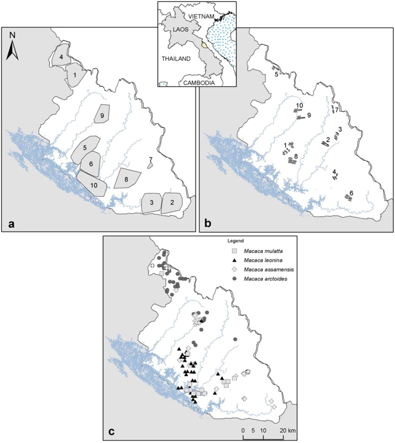
Figure 1.
(
a) Camera-trap sampling effort from 2006–2011 (sampling areas obtained with a minimum convex polygon around camera-traps set;
cf. Table 1); (
b) transect surveys from 2011–2012, total km walked, including replications are presented in
Table 1; (
c) Macaques species occurrence localities used for the models.
2.3. Species Distribution Modelling
To model the potential distribution and niche of macaque species in NNT NPA, we used the maximum entropy general purpose machine learning method, which has been adapted and developed as a software (MaxEnt) for species distribution modelling [
24,
25] and identified as one of the best methods for species niche modelling [
26]. MaxEnt version 3.3.3k is used to perform the analysis (
http://www.cs.princeton.edu/~schapire/MaxEnt/). The method combines biological data of species occurrence (presence-only data) with environmental characteristics (e.g., GIS layers with a grid of values for the geographic area considered) to estimate the probability distribution of maximum entropy (
i.e., closest to uniform), subject to the set of constraints provided (
i.e., environmental characteristics where the species occurs) [
25].
2.5. Model Evaluation
We assessed the performance of our models using four methods: (i) the area under curve (AUC) of the receiver-operating characteristic (ROC) (ii) the use of a null-model [
29], (iii) the Boyce Index method [
30], (iv) and the jackknife validation method [
31] for our smallest sample only. In addition, results outputs are interpreted in term of known ecology of the study species at National scale, published by experts (
cf. Discussion section).
The AUC of ROC is provided in the model outputs. It is obtained by plotting
sensitivity on the x-axis and 1-
specificity on the y-axis, with
sensitivity representing the proportion of correct prediction of actual presence (true-positive, or absence of omission), whereas 1-
specificity is the proportion of falsely predicted presence (false-positive, or commission error) for all possible thresholds of the probability (threshold independent evaluation). In presence-only models, the AUC value represents the probability that the model scores a presence site (test locality) higher than a random background site [
25]. The value ranges from 0.5 to 1−
a/2, where
a is the fraction of pixels covered by the species’ distribution that remains unknown, thus renders inadequate the interpretation of AUC [
25,
29,
32]. Nevertheless, it remains the most commonly used evaluation parameter and is presented here. An AUC value closer to 1 indicates that the model predicts better than random, while a value of 0.5 indicates that the prediction is no better than random [
25].
Given the recent critics of using AUC for presence-only model evaluation [
29,
32], we used other methods to evaluate the performance of the model outputs. A recently developed alternative is the null-model, which was introduced by Raes and Steege [
29]. The method tests the AUC value of the model against a null distribution of expected AUC values based on random occurrence data from the geographic area considered. More concretely, it tests if the relations between species occurrence and environmental variables at these locations are stronger than expected by chance [
29]. The exact same number of occurrence points available for each species (48, 38, 34 and 14;
cf. Table 2) were randomly drawn across NNT NPA and replicated 999 times. These null-distributions were run separately in MaxEnt with the same settings detailed above. This resulted in 999 AUC values of the null-model for each of the four species. AUCs of the null-models were ranked and the position of the real species’ AUC was tested against the 95% confidence interval (CI) of the null-model’s AUC values. The species’ model is considered performing better than expected by chance if its AUC value is ≥95% CI null-model’s AUCs [
29].
In addition, we apply the Boyce Index validation method [
30,
33] to our models. The continuous habitat suitability scores obtained from the outputs (0 to 1) are reclassified into a number
i of bins (classes). For each class, two frequencies of pixels are calculated: the Predicted Frequency and the Expected Frequency. The Predicted Frequency is the number of occurrence points predicted by the model falling into in the class
i divided by the total number of occurrence points. The Expected Frequency is the number of grid cells included in class
i, divided by the total number of grid cells in the whole geographic area considered. A Predicted-to-Expected ratio is calculated for each class and a Spearman rank correlation coefficient
rho (1-tailed test) evaluates if the ratio significantly increases as suitability increases (
p < 0.05) [
33]. Our models’ outputs were reclassified into 100 continuous classes of equal interval and we calculated a P/E ratio for each class. Statistical tests were performed with SPSS.v.17.
Finally, for the smallest sample (
M. mulatta;
n = 14), we followed the jackknife validation method for samples
n < 25 described by Pearson
et al. [
31], in which it is assessed if the model successfully predicts the n left-out localities (one locality at each of the 14 replications) within the area of suitability (under the minimum training presence threshold chosen). This is assessed with a pValue based on the test statistic
D;
D = ΣX
i (1 − P
i), where X
i is the success-failure variable indicating if the
ith left-out locality is included or not in the predicted area and P
i is the probability of success [
31]. The pValue is computed with
pValue compute program [
31].
2.6. Output Analysis
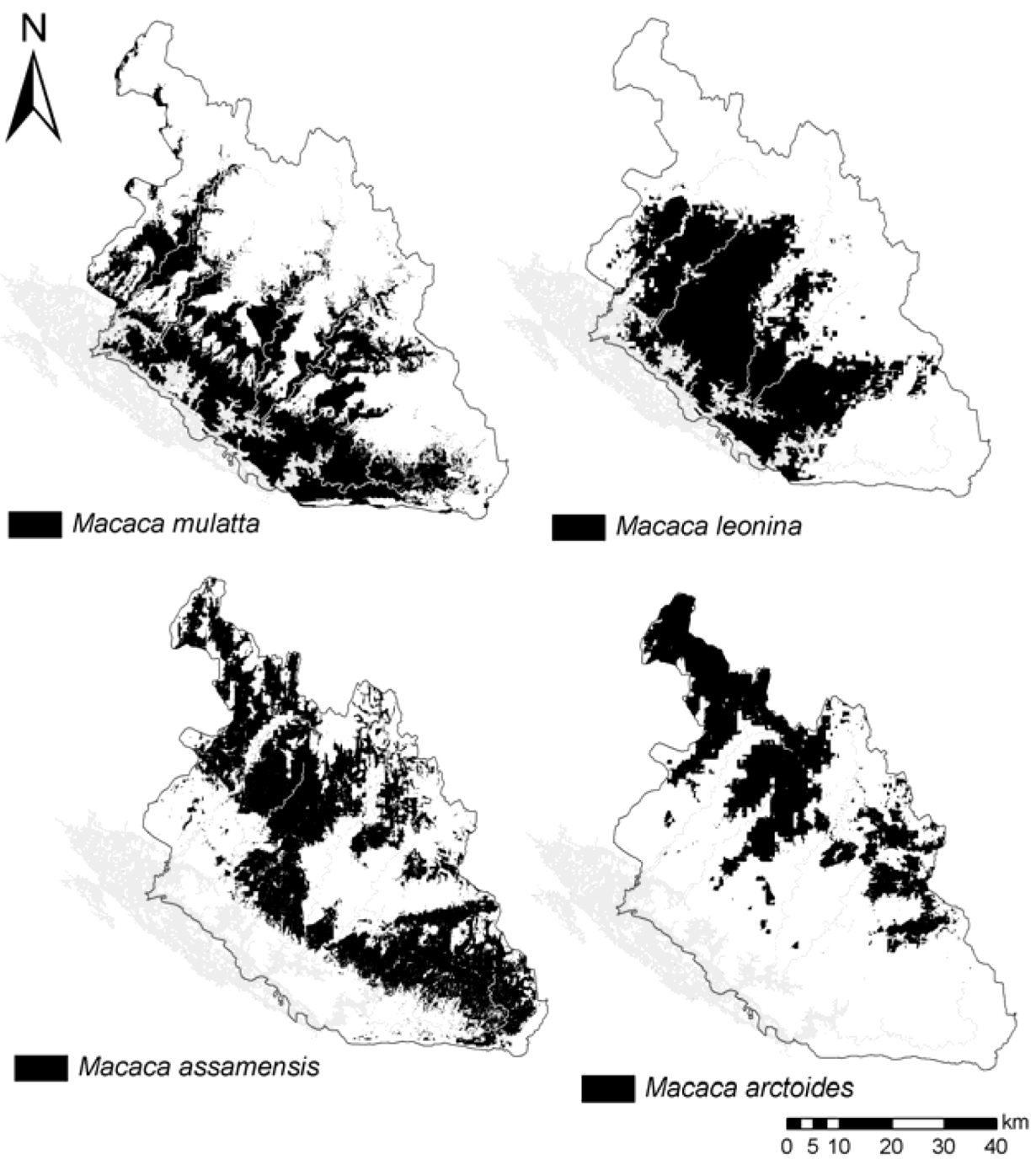
To produce a binary map (
i.e., suitable
vs. non-suitable habitat), we used the “
minimum training presence logistic” threshold, which has been commonly used when occurrence data are highly reliable, such as here, given the confirmed species identification and records in their primary habitat. This threshold has the advantage to maintain zero omission error and include all areas that are at least as suitable as those where the species is known to occur [
31,
34]. The final potential distribution for each species was projected (WGS 1984 UTM Zone 48N) in ArcGIS 9.3.
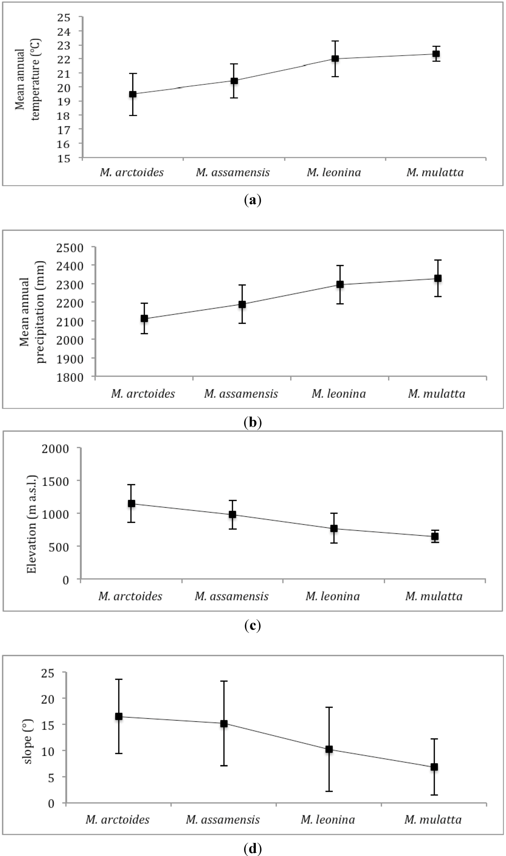
We calculated mean values of environmental variables within the predicted distribution of the four species. Predicted suitable habitat of the four species is also tested pair-wise for their similarity using two different statistical tests that compare the logistic habitat suitability scores provided in MaxEnt’s model outputs: Schoener’s D [
35] and
I statistic [
36]. Their value ranges from 0 (no overlap in habitat suitability) to 1 (complete overlap in habitat suitability); they are calculated using the ENMTool [
36]. Range overlap is also quantified with ENMTool with the formulae (N
x,y/min[N
x, N
y]), where N
x,y is the number of grid cells where both species x and y are predicted to occur and N
x and N
y are the number of grid cells where respectively species x and y are predicted [
36]. We apply a threshold at which habitat is considered suitable, using the average of all four species’ “Minimum training Presence logistic” threshold (=0.171).


