1. Introduction
Accurate information about the distribution of species is essential for their conservation and management [
1]. Without this vital information, the species may not be considered when impacts of habitat alterations or other actions are considered for an area, or conservation and management efforts could be directed at areas where the species does not occur. Yet, in most cases species occurrence can only be sampled and hence distributions must be extrapolated. Traditionally, such extrapolation was accomplished via gestalt by a taxon expert, such as might be presented in a floral or faunal monograph [
2]. However, the recent advent of niche-based species distribution modeling has provided rigorous quantitative means for extrapolating beyond known occurrence points [
3,
4]. These methods are attractive because they not only allow for habitat suitability of the organism to be predicted and mapped, but, they also allow for extrapolation of predicted occurrence beyond the study area and they provide information about the relationship between the species and the environment [
5]. And yet, even these robust methods must be based on the fundamental underlying occurrence data, which are subject to a spectrum of errors.
Frey [
2] provided a review of the nature of occurrence records, including types, problems with interpretation, and reasons for data gaps. Briefly, the most unambiguous type of occurrence record is based on preserved physical evidence, such as a museum voucher specimen, although even these can introduce error [
2]. Other types of occurrence records are based on more equivocal forms of evidence, such as field observations of an animal or its sign. Because they cannot be independently verified, such records are considered anecdotal [
6]. Occurrence records are subject to three dimensions of errors: the accuracy and precision of the spatial location, the spatial sampling of the records, and the reliability of the report. There has been a variety of recent studies that have evaluated the impact of spatial errors and bias on presence-only species distribution models (SDMs), which in general have found many methods to be robust, such as those based on maximum entropy [
3,
7,
8,
9,
10,
11].
In contrast to spatial errors, the impact of the reliability of occurrence records on the interpretation of species distributions has received little attention [
1,
2,
6,
12]. Although Lozier
et al. [
12] provided an extreme example of the problem of misidentification by comparing SDMs of the cryptozoid Sasquatch and the American black bear (
Ursus americanus) and concluded that records of Sasquatch were a case of misidentification, no studies have evaluated influence of different severities in error of reliability on niche-based SDMs. Reliability refers to the degree to which an occurrence record can be trusted to be accurate. Thus, reliability primarily refers to the accuracy of the species’ identification [
2,
6], although it also may include potential for deceitfully manufactured information. Frey [
2] presented a scheme of seven classes, ranging from verified to erroneous, for evaluating the reliability of species occurrence records (
Table 1). In this scheme, most of the classes (
i.e., B-F) are anecdotal records. The scheme was based on three criteria that can influence accurate identification of a species, including observable diagnostic characteristics of the species, environmental conditions during the observation, and the observer’s knowledge about diagnostic characters of alternative potential species [
2]. Consequently, an occurrence record would have a lower probability of reliability if it is of a cryptic species, observed during poor conditions (e.g., animal moving through shrubs at night), or made by a novice observer. Yet, while reliability reflects the inherent essence of an occurrence record, rarely has it been explicitly considered during distributional analyses [
2,
13,
14]. Most commonly, all accumulated occurrence records are included in distribution analyses or modeling without regard to possible deficiencies in reliability. Thus, species distribution modeling typically proceeds by implicitly assuming that all records are reliable. This problem is likely heightened due to the increasing availability of large networked species occurrence data sets (e.g., Global Biodiversity Information Facility, NatureServe).
McKelvey
et al. [
1] argued that the use of anecdotal data to infer species distributions for rare or elusive species can lead to substantial errors, which can have profound negative impacts on conservation. For example, they found that overestimating species ranges due to accepting erroneous records caused underestimation of extent of range losses resulting in a delay in conservation actions for the fisher (
Martes pennanti) in the Pacific states, failure to recognize historical isolation and extirpation of the wolverine (
Gulo gulo) in California resulting in an underestimation of loss of diversity and distribution in this species, and “resurrection” of the extinct ivory-billed woodpecker (
Campephilus principalis) in the southeastern United States resulting in the expenditure of funds on costly conservation measures that otherwise could have been spent on species verified as extant. They argued that the proportion of false positive records will be higher for rarer species. Thus, they suggested that higher evidentiary standards based on verifiable data be used for determining the distribution and status of rare or elusive species.
The overarching goal of this study was to explore how datasets of occurrence records that differ by inclusion of various classes of reliability influence the interpretation of the distribution of an elusive carnivore, the white-nosed coati (
Nasu narica), in the American Southwest. The coati is morphologically and behaviorally (e.g., arboreal, diurnal, gregarious, vocal) distinctive and hence not likely to be misidentified by experienced biologists in the American Southwest [
15]. The species reaches its northern range limits in southwestern New Mexico and southeastern Arizona [
15]. However, due to apparent rarity or elusiveness, the status and distribution of coatis in the region has been a matter of long-running conjecture [
16,
17,
18,
19,
20,
21,
22,
23,
24,
25]. For example, in New Mexico it is currently known by only two specimens [
26], while in Arizona numerous records in the central part of the state have been considered to represent wanderers [
21,
22].
Table 1.
Classes for evaluating the reliability and precision of occurrence records for the white-nosed coati (
Nasua narica) in Arizona and New Mexico. Reliability classes were adapted from Frey [
2].
Table 1.
Classes for evaluating the reliability and precision of occurrence records for the white-nosed coati (Nasua narica) in Arizona and New Mexico. Reliability classes were adapted from Frey [2].
| Class | Characteristics |
|---|
| Reliability |
| A | Verified: An expert’s evaluation of preserved physical evidence, including photographs. |
| B | Highly Probable: An expert’s accurate observation, but no physical evidence is preserved. |
| C | Probable: A first-hand report of an observation that is likely to be accurate. Convincing details are provided. |
| D | Possible: A potentially inaccurate observation made by an expert due to poor conditions. |
| E | Questionable: First-hand report of a potentially inaccurate observation because of the observer’s lack of knowledge, suboptimal observation conditions, or the lack of supporting details, this class is not as convincing as class C. |
| F | Highly Questionable: Records that have a high potential of inaccuracy. Includes second-hand and unpublished reports. |
| G | Erroneous: Physical evidence verifies the reported species was misidentified. |
| Precision |
| H | Actual location likely <30 m of coordinate |
| I | Actual location likely 30–500 m of coordinate |
| J | Actual location likely 500–1,000 m of coordinate |
| K | Actual location likely 1,000–2,000 m of coordinate |
| L | Actual location likely 2,000–3,000 m of coordinate |
| M | Actual location likely >3,000 m of coordinate |
3. Results
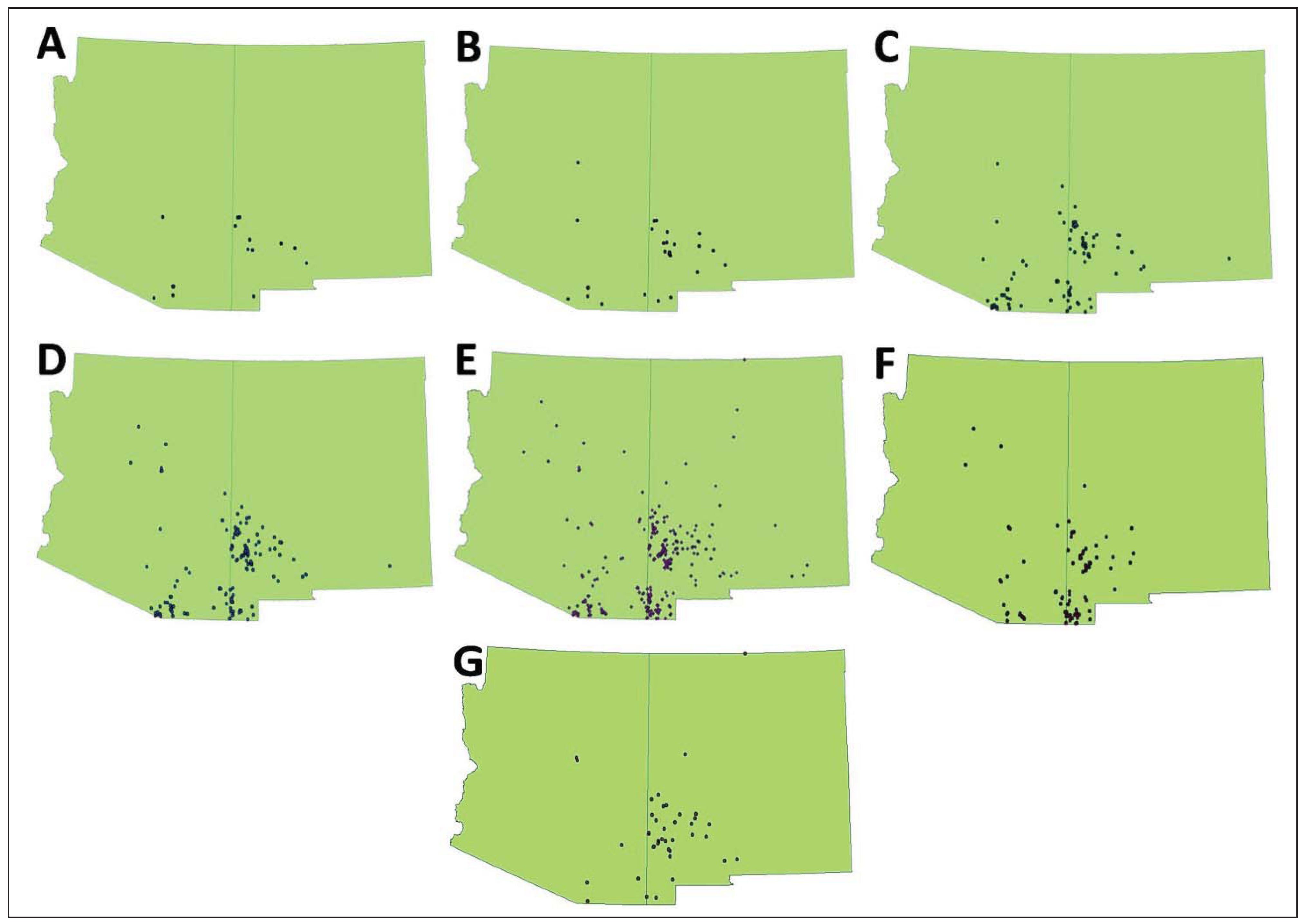
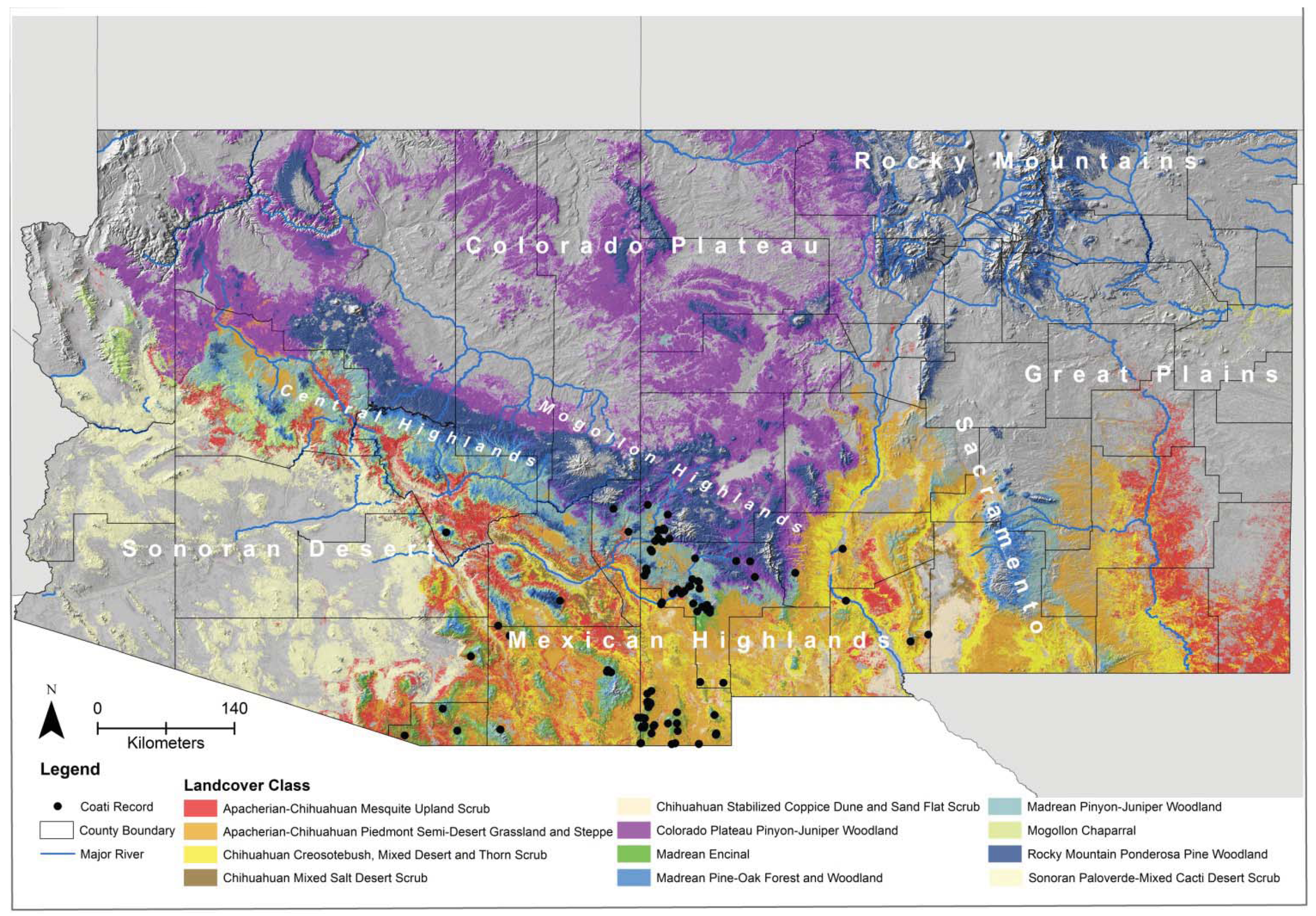
We obtained 317 unique occurrence records for
N. narica (
Table 2,
Figure 1). Only one dataset (very conservative) had a small sample size (
i.e., <30 records), which can cause potential inaccuracies in SDMs [
10,
37]. All other models had adequate or large sample sizes (
i.e., >100 records) [
10]. Further, 94.3% of records were from 1950 or later (79.2% since 1990) and hence the vast majority were within the time frame of the climate and land-cover data. All bioclimatic and biophysical ENMs had high (
i.e., >0.90) AUC
test values except the very conservative and poor reliability biophysical models (models 8 and 13;
Table 3,
Table 4). For both the bioclimatic and biophysical ENMs the best performing models were those that included a low to moderate classes of error in reliability and precision, with the best a priori model performing best. Model performance declined with either decreasing sample size (the very conservative and conservative models) or increasing error (liberal model). While the poor precision model performed almost as well as the best a priori model, the poor reliability model was the worst performing model.
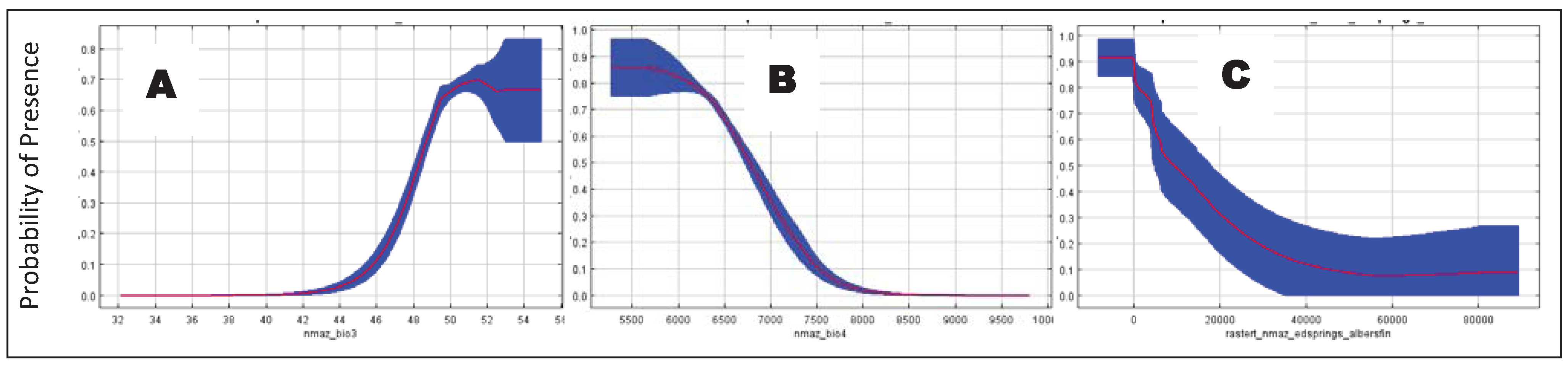
For the bioclimatic ENMs, isothermality (
i.e., Bio 3) had the highest variable contribution in all models, except model 7 (
i.e., poor precision model;
Table 3). Other variables with significant contributions (
i.e., >5%) in most models (
i.e., models 2–5) included: mean temperature of the driest annual quarter (Bio 9), precipitation and temperature seasonality (Bio 15 and 4, respectively), and precipitation of the coldest and wettest quarters (Bio 19 and 16, respectively). The poor precision model (model 7) was similar in variable contributions to these models with exception that mean temperature of the wettest quarter (Bio 8) was also important. In contrast, the very conservative (model 1) and poor reliability (model 6) models markedly departed from these patterns in idiosyncratic ways. Regardless of the datasets used, the jackknife tests indicated that isothermality (Bio 3) and temperature seasonality (Bio 4) were always the first or second most important variables.
For the biophysical ENMs, with a few exceptions, all variables were significant (>5%) contributors to all models (
Table 4). The highest variable contributions in all but one of the biophysical models were land-cover and distance to springs, which together ranged from 55–78% of contribution to those models. The exception was the conservative model (model 9), wherein road density had the highest variable contribution and land-cover had the lowest contribution. In other models, road density was <14% contribution. The jackknife tests indicated that land-cover type, followed by distance to springs, were the most important variables (except for in the conservative model where road density was the second most important variable). Land-cover types with the highest suitability for coatis included Madrean encinal, Madrean pinyon-juniper woodland, and Mogollon chaparral, despite these accounting for only 21.4% of the area of suitable habitat (
Table 5).
Table 5.
Mean suitability of important land-cover types for the white-nosed coati (
Nasua narica) in Arizona and New Mexico based on the best
a priori set of occurrence records (see
Table 3,
Table 4). Only land-cover types accounting for >1% area of suitable habitat are included.
Table 5.
Mean suitability of important land-cover types for the white-nosed coati (Nasua narica) in Arizona and New Mexico based on the best a priori set of occurrence records (see Table 3, Table 4). Only land-cover types accounting for >1% area of suitable habitat are included.
| Land-cover type | Proportion of area of suitable habitat (%) 1 | Mean habitat suitability (%) |
|---|
| Madrean Encinal | 6.3 | 47.1 |
| Madrean Pinyon-Juniper Woodland | 12.6 | 40.7 |
| Mogollon Chaparral | 2.5 | 38.8 |
| Chihuahuan Mixed Salt Desert Scrub | 2.5 | 34.7 |
| Madrean Lower Montane Pine-Oak Forest and Woodland | 1.4 | 34.6 |
| Apacherian-Chihuahuan Mesquite Upland Scrub | 10.6 | 22.6 |
| Apacherian-Chihuahuan Semi-Desert Grassland and Steppe | 28.2 | 18.9 |
| Chihuahuan Creosote, Mixed Desert and Thorn Scrub | 10.4 | 16.7 |
| Southern Rocky Mountain Ponderosa Pine Woodland | 8.5 | 14.6 |
| Colorado Plateau Pinyon-Juniper Woodland | 5.1 | 13.9 |
| Chihuahuan Stabilized Coppice Dune and Sand Flat Scrub | 1.2 | 8.3 |
| Sonoran Paloverde-Mixed Cacti Desert Scrub | 2.8 | 5.9 |
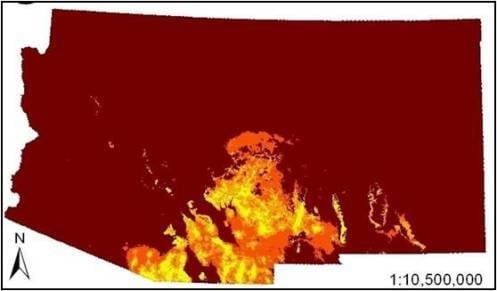
The SDMs (
i.e., combined bioclimatic and biophysical ENMs) predicted occurrence of coatis primarily in southeastern Arizona and southwestern New Mexico (
Figure 2). There was minor variation in the spatial models. For example, the model that visually departed from the others the most was the very conservative model, which predicted occurrence of coatis in the Arizona Central Highlands, which is a northwest trending mountainous region south of the Colorado Plateau in central Arizona. The liberal model slightly differed mainly in predicating mid elevations of mountain ranges and escarpments in southeastern New Mexico. However, percent similarity between the very conservative SDM and all other SDMs based on less reliable datasets were all very high (94% to 96.1%). In addition, the AUCs among all pair-wise comparisons of models within the bioclimatic or biophysical sets were not significantly different (
P > 0.05), with exception of a comparison between the most dissimilar bioclimatic models (
i.e., very conservative model
versus moderate model;
Z = 2.678,
P = 0.008).
Figure 2.
Species distribution models (
i.e., combined bioclimatic and biophysical ecological niche models (ENMs)) for the white-nosed coati (
Nasua narica) in Arizona and New Mexico based on different subsets of occurrence records (see
Table 3,
Table 4): (
A) very conservative, (
B) best a priori, and (
C) liberal.
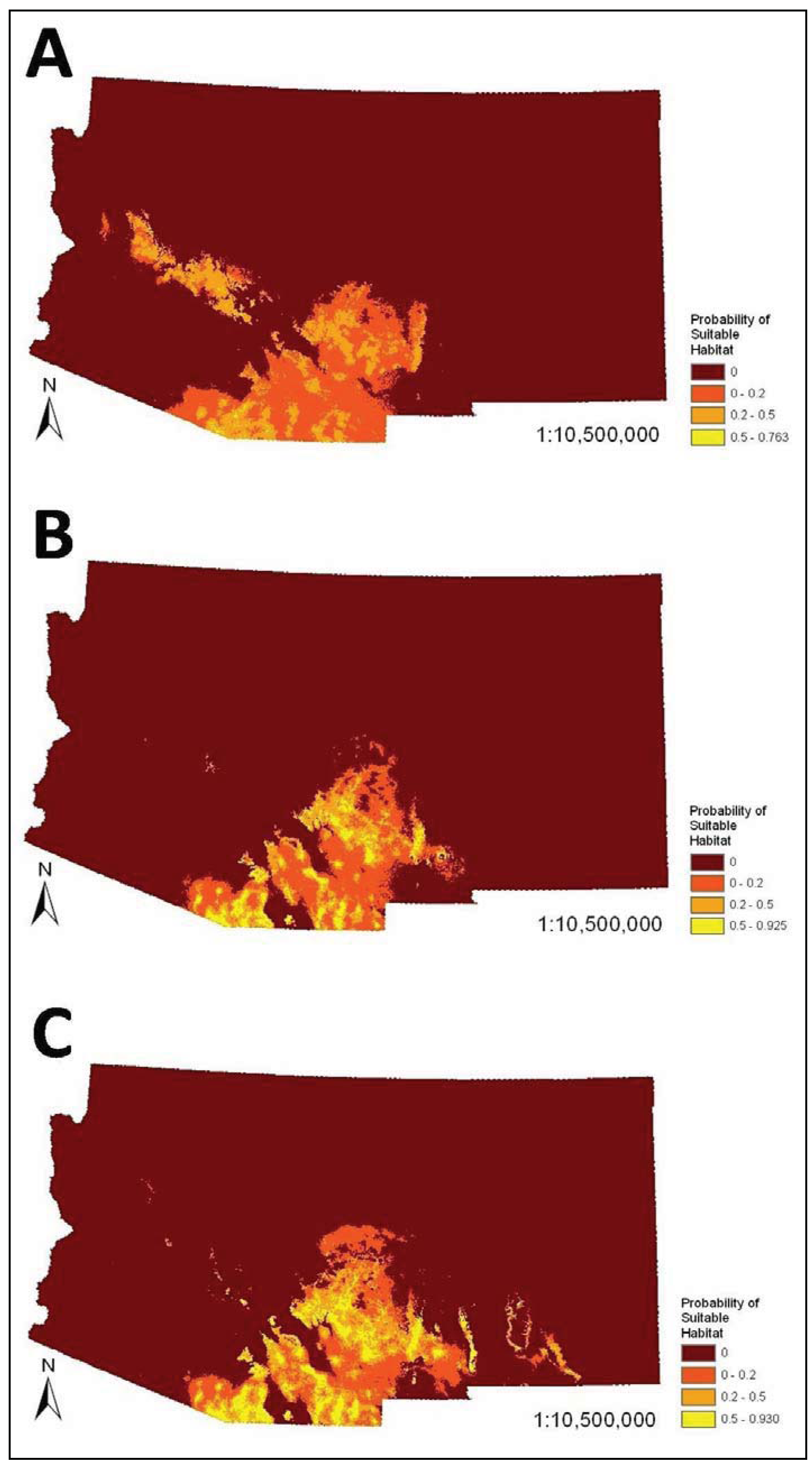
5. Conclusions
This study is the first to evaluate the impact of reliability of occurrence records on niche-based species distribution models. We found that for the white-nosed coati, inclusion of anecdotal records provided similar results compared to those based only on verified records. Thus, field observations may provide an important source of data for understanding the distribution of many rare species where there is a paucity of physical evidence. This is important because anecdotal data can provide some benefits over physical evidence such as being relatively inexpensive, abundant (possibly providing better geographic coverage), and derived from multiple sources (possibly negating some sampling biases). In contrast to McKelvey
et al. [
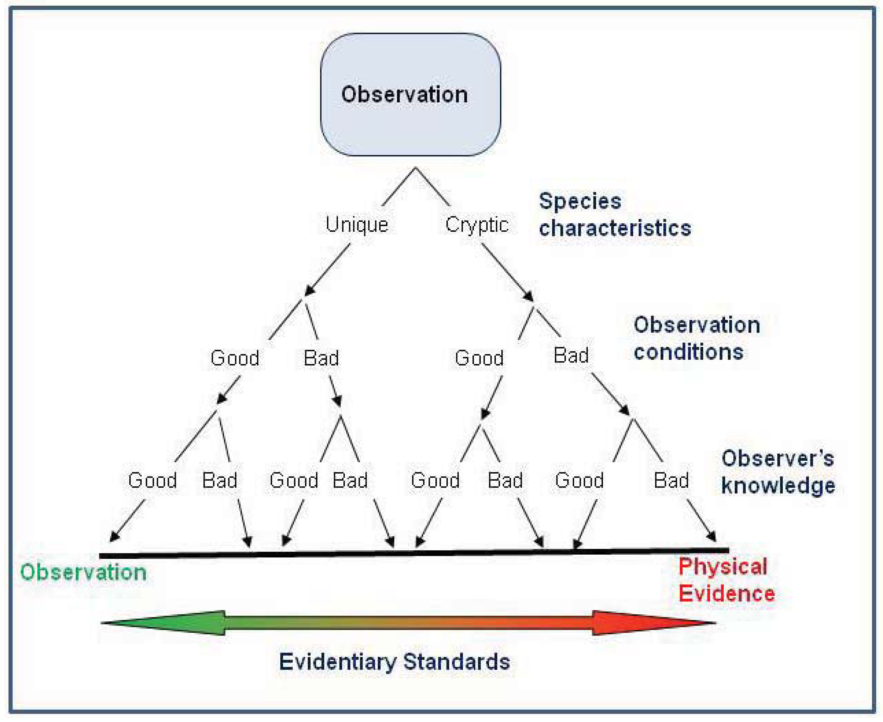
1] who suggested that higher evidentiary standards should used for determining the distribution and status of rare or elusive species, we believe that higher evidentiary standards are required for species that pose identification problems, and where observation conditions or observer knowledge are poor (
Figure 5). However, we strongly caution that our results may not be applicable to all situations. We recommend that anecdotal occurrence records only be used according to the following criteria: (1) Maximum entropy methods should be used to infer distributions based on anecdotal data because the algorithms assign low probabilities to unusual occurrences. (2) Occurrence records should be evaluated for their reliability with only the most reliable used for interpreting distribution. (3) Anecdotal records should be used to supplement (not in lieu of) physical evidence. (4) Species must exhibit readily observable diagnostic features; cryptic species require either physical evidence or observation and verification by a taxon expert. Lastly, we urge for additional research on the influence of the reliability of occurrence records on species distribution models, especially using simulation data and making comparisons among species that vary in ease of identification and comparisons among different demographic groups of observers (e.g., experts
versus naïve).
Figure 5.
Scheme of evidentiary standards for occurrence records based on the species characteristics, observation conditions, and observer’s knowledge. The highest evidentiary standards (i.e., requiring physical evidence) are necessary when the species poses identification problems or when observation conditions or the observer’s knowledge are poor. In contrast, anecdotal evidence might be acceptable for interpreting distribution if the species has readily observable diagnostic features, especially if observation conditions allow evaluation of the diagnostic features, or the observation is made by a taxon expert.


