Geotechnical Analysis and 3D Fem Modeling of Ville San Pietro (Italy)

Abstract

The paper describes the three-dimensional numerical model of Ville San Pietro, an Italian village subject to slope movements causing damage. The church (dating back to 1776), which is the most significant building of the area, is modelled too. The information from geotechnical and geophysical surveys on field are used to define the model geometry and the soil properties. A finite element code is adopted to simulate the slope behavior in occurrence of water table fluctuations, detected by piezometers, and to evaluate the slope displacements and stability. The validation of the model is carried out using the inclinometer and interferometry measures and by on-site inspections. The model demonstrated a good ability to simulate the slope behavior during the raising and lowering of the water table. The critical areas computed by the numerical code are in good accordance to the actual portions affected by soil displacements and damages. The modelling presented in this paper is crucial for future analyses that will take advantage of an innovative monitoring system, which will be installed on site.

1. Introduction

Landslides are common and widespread phenomena in Italy and around the world. Each year, they cause damage to the population and very serious economic and environmental problems. Hence, the slope stability monitoring and the landslide risk mitigation are primary scientific and social targets in order to improve the resilience of our territories.

Landslides occur in a given area due to the concomitance of various factors (anthropic, geological, hydrological, etc.). In general, the rainfall is the main landslide triggering factor.

The LAndslide Monitoring and Predicting (LAMP) system, proposed in an INTERREG-ALCOTRA project called AD-VITAM (“Analisi Della Vulnerabilità dei Territori Alpini Mediterranei ai Rischi Naturali”), is formulated for the analysis and forecasting of landslides (more specifically debris and earth slides) triggered by rainfalls [1]. LAMP adopts an Integrated Hydrological Geotechnical (IHG) model [2,3], implemented in Geographic Information System (GIS) environment for three-dimensional slope analyses. The IHG model is fed by data measured by a Wireless Sensor Network (WSN) composed of low-cost self-sufficient sensors. WSN observes rain, temperature, displacements and even the soil moisture. Multiple installations (along vertical alignments) of capacitance sensors are placed at the nodes of the monitoring network. They provide real-time water content profiles in the shallow layers (typically in the upper meter) of the slope. The capacitance sensors (more specifically, WaterScout SM100 sensors, manufactured by Spectrum Technologies, Inc., Plainfield, IL, USA) are appropriately calibrated by laboratory tests in order to define soil-specific calibration curves [4,5]. There are several reasons why capacitance sensors are used to measure the soil moisture in the LAMP system. The knowledge of soil water content variability in space and time is necessary for:

• The hydrological–geotechnical analysis;
• The study of the hydro-mechanical contribution from the vegetation and, eventually, for a landslide risk mitigation by using soil bio-engineering countermeasures. In fact, the relevance of the contribution of plant roots to prevent the instability and the soil erosion has been long observed and it is recognized [6,7,8,9];
• The hydro-geological risk management. In fact, it is well known that landslide risk conditions persist for long after the officially issued alert has been ceased. For instance, by monitoring the soil water content, it would be possible to understand when people, subject to removal, can return to their homes safely.

The final products are maps of landslide susceptibility (in raster format), both for measured and, if needed, forecasted rainfalls.

AD-VITAM aims to improve the resilience of territories subject to landslide risk: in particular, it studies the evolution of the relationship between rainfall and slope stability for an affective analysis and mitigation [10]. The ALCOTRA cooperation program covers the area between Italy and France (Piedmont, Liguria, Valle d’Aosta and Provence-Alpes-Côte d’Azur-PACA). Among the sites of interest, there is Ville San Pietro (Liguria-Italy). This paper is aimed at describing the first three-dimensional model of Ville San Pietro ever made.

The modelling here presented is crucial for future analyses that will take advantage of the LAMP monitoring system. In fact, the numerical modeling of Ville San Pietro has several purposes:

• Preliminary study of the site;
• Identification of the places where the nodes of the LAMP network should be positioned;
• Comparison with IHG analyses based on monitoring measures.

Nowadays, numerical methods represent the most comprehensive calculation tools for geotechnical analyses. They are very used for practical and research studies, due to the possibility of simulating realistic geometries and the interaction between structural elements and soil, whose behavior can be described by several constitutive models.

Many authors have shown the disadvantages and advantages of three-dimensional (3D) over two-dimensional (2D) analyses with reference to various geotechnical engineering problems [11,12,13].

As known, a two-dimensional numerical model represents a simplification of the real problem, which is analyzed only at one or some representative cross-sections. This approach is generally adopted for many engineering applications. However, 2D analyses do not really simulate the complex behavior of landslides, composed by parts with different sliding directions and velocities.

Geotechnical engineers still not routinely perform three-dimensional slope stability analyses even though most slope stability problems are clearly three-dimensional. 3D analyses by Finite Element Method (FEM) codes are rarely conducted in routine geotechnical design, due to the complexity of the numerical modeling with regard to the geometry, the determination of the material parameters, and above all, the time consumption for calculation. Moreover, it is commonly believed that 2D slope stability analyses provide more conservative estimates of the 3D slope stability problem. For instance, Duncan [14] reported that a conservative result can be obtained if the most pessimistic section of a 3D slope is selected for 2D analyses. However, the most pessimistic section of a slope may not be intuitively evident [15], especially for cases with random soils. Griffiths et al. [16] underlined that the 2D analysis does not necessarily ensure a conservative result than the 3D analysis. This finding underscores the necessity of 3D analyses for slopes with random soils [17], complex geometries, general loads and conditions. Quite recently, 3D FEM analyses have been performed for slope stability estimates, showing the effectiveness of this approach and its suitability for complex models [18,19].

In general, stratigraphy has an important role in the slope analysis. However, in most cases, only a small amount of data are available and, consequently, the stratigraphy is necessarily simplified in the modelling. In fact, it is common practice to neglect the relatively thin or discontinuous layers, remedying with a proper calibration of the parameters, based on monitoring data [20]. Calibration and validation are certainly delicate and crucial phases in the modeling.

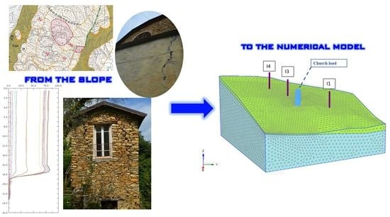
The 3D finite element numerical model described in this paper is rather uncommon because of its extent and relevant discretization. Besides, the church is included in the 3D model of Ville San Pietro, since it is the most significant building from the historical and cultural point of view, the most damaged and certainly, the most considerable with reference to the load applied to the ground.

The slope response to observed water table fluctuations is simulated and stability analyses are performed to define the areas prone to movements. Inclinometer and interferometry data and on-site inspections testify to the effectiveness of the model in simulating the behavior of the slope.

Moreover, by exploiting the numerical analyses shown in this paper, it was possible to define the positioning of the monitoring network in Ville San Pietro.

2. Materials and Methods

2.1. Ville San Pietro: Location, Description of the Landslide, Investigations and Monitoring

2.1.1. Site and Landslide Description

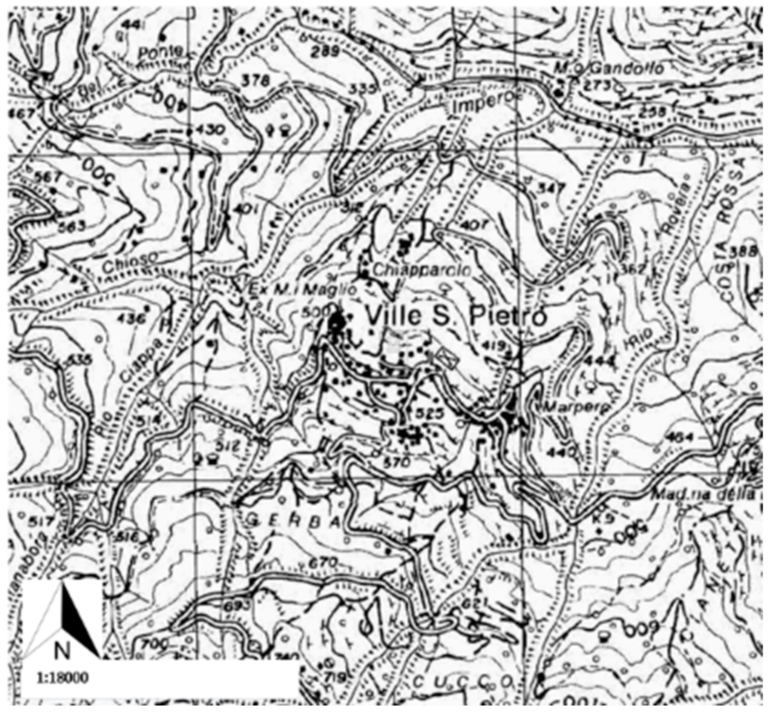
Ville San Pietro is a small village in Liguria (Italy) situated at about 500 m a.s.l. on the right of the Impero River (Figure 1).

The area of Ville San Pietro is entirely characterized by the presence of Sanremo Flysch, belonging to the Sanremo-Monte Saccarello Tectonic Unit.

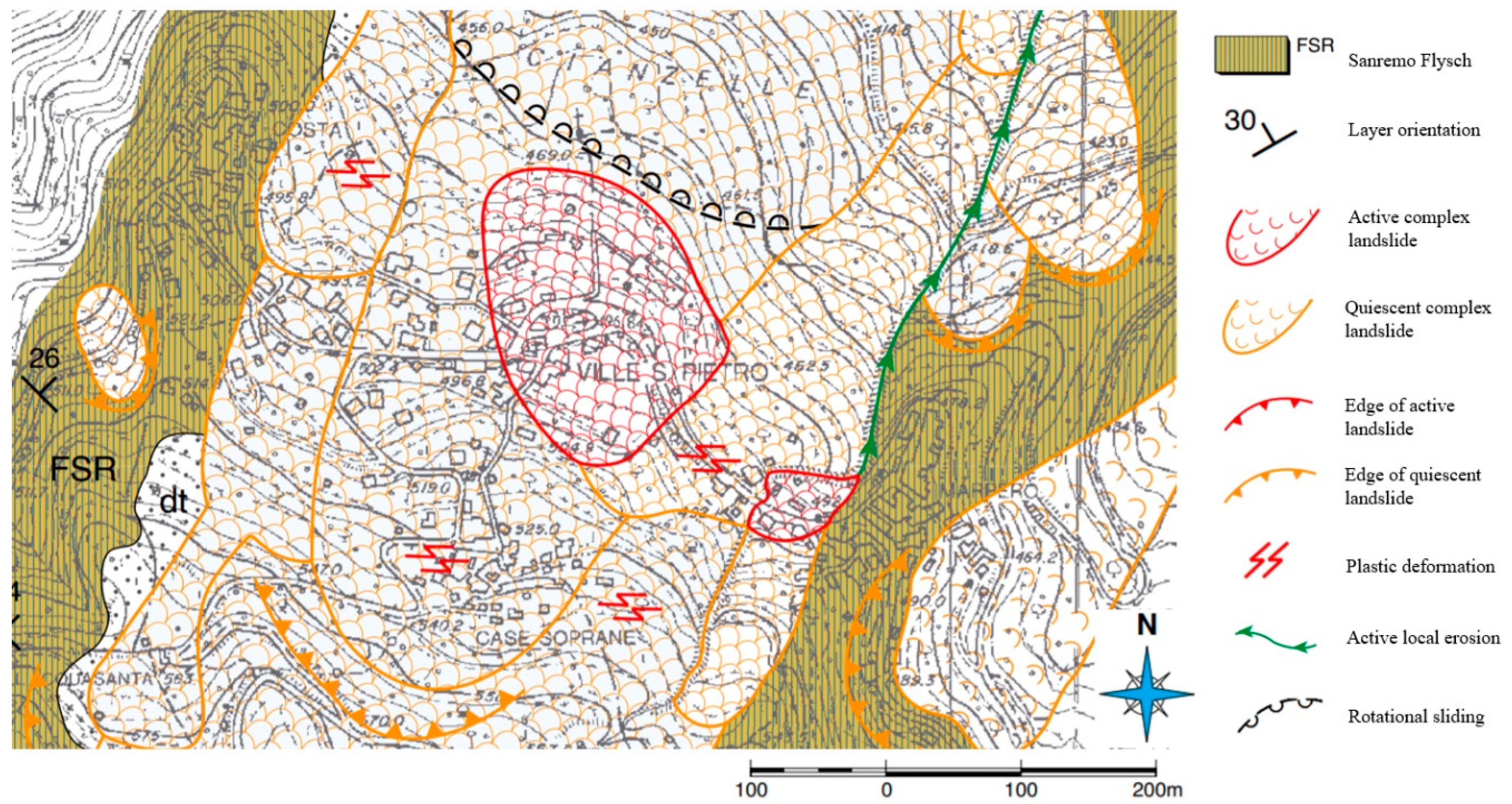
The slope is classified by the Italian Landslide Inventory (Inventario dei Fenomeni Franosi in Italia (IFFI)) as a large complex relict landslide (length: 1500 m; width: 500 m; average thickness: 15 m; volume: about 11 × 10⁶ m), suffering reactivations over time (Figure 2). Typical phenomena are falls (where there are rock outcrops), slides and flows (in the shallow blanket that characterizes the area).

A thick debris blanket features the site; a bedrock, formed by prevalent limestone with presence of marl and sandstone, lies below. The presence of clay has an important role on the activation of the landslide. In this way, the shear band generally occurs at narrow clayey layer between the main one. The application of loads due to new constructions and the inadequate water regulation on the slope are responsible of instabilities, too. Rather slow soil displacements cause damages to the structures built on the slope (e.g., the buildings, the church and the retaining walls).

Since 2008, Ville San Pietro has been monitored by piezometers and inclinometers in order to observe both water table fluctuations and soil displacements.

2.1.2. Geotechnical Surveys

Geotechnical surveys allow the definition of the geotechnical model of the subsoil and are of fundamental importance for any site analysis.

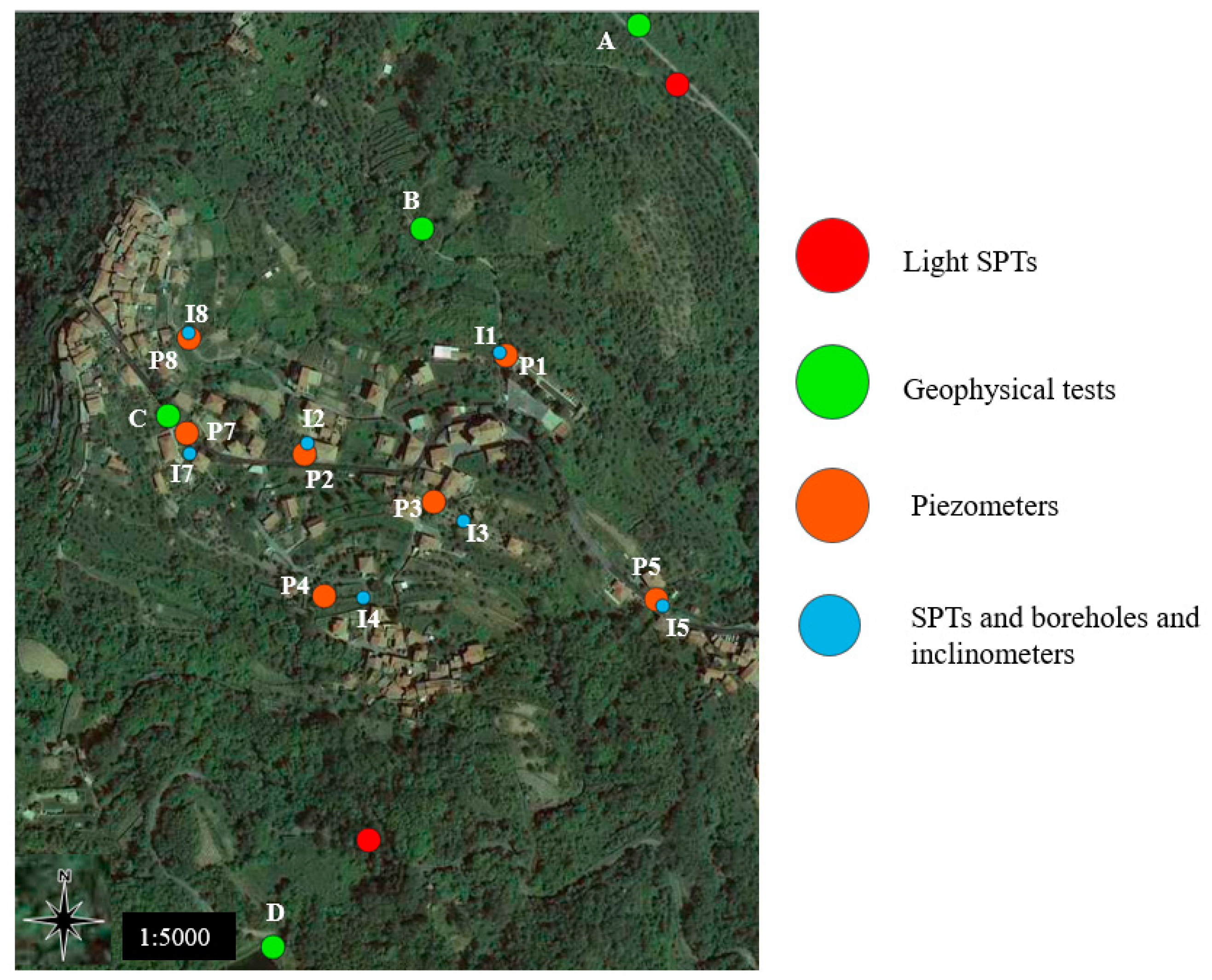
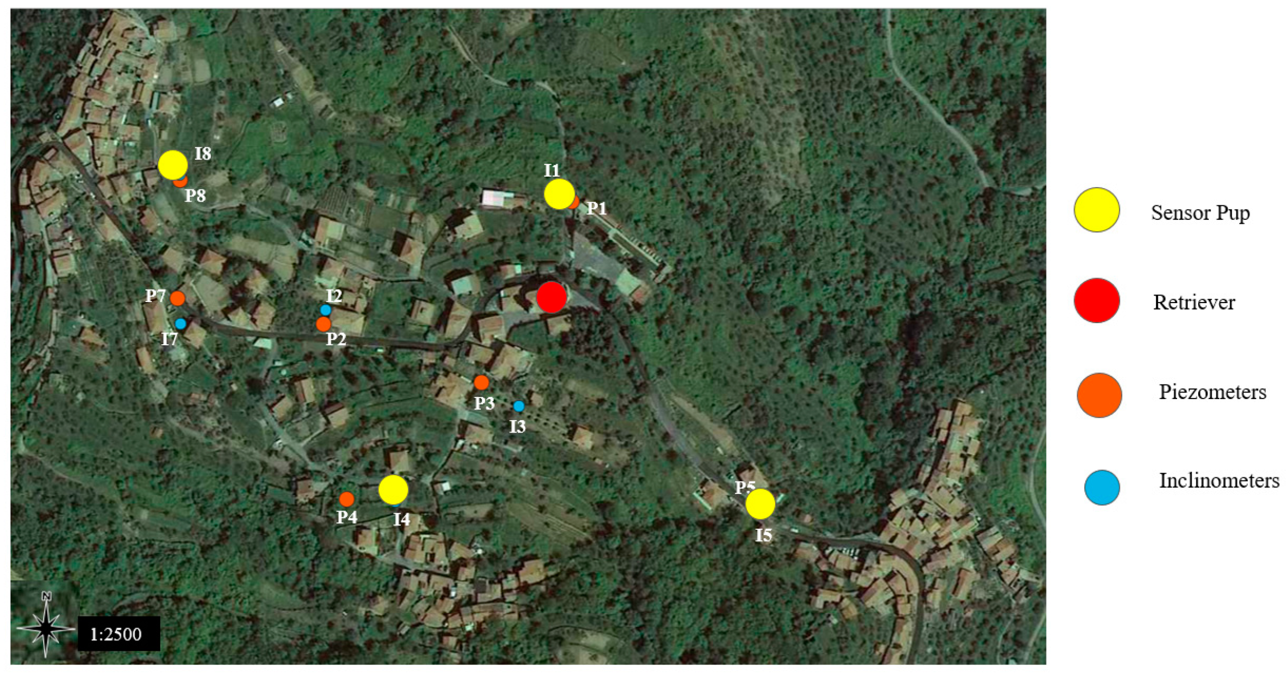
In 2002, five boreholes and five Standard Penetration Tests (SPTs) were performed in Ville San Pietro. In 2008, two boreholes were added. All the boreholes were equipped with inclinometers and piezometers were installed in their proximity (Figure 3).

The rotation and destruction drillings were executed by a hydraulic drilling machine Beretta T44, mounted on mechanical tracks. The characteristics of this device are rotation velocity 550 rpm, maximum torque 650 kg·m, push 4000 kg, pressure of the pump 50 bar and flow 200 L. The drill was performed with a tri-cone bit (diameter 114 mm). The boreholes lacked of self-maintenance so they were covered with steel pipes during the perforation.

As shown in Figure 3, these points (represented by blue and orange dots) are located in the middle of the slope. This zone is in fact of great interest as it is affected by slope movements and here the structures are consequently damaged.

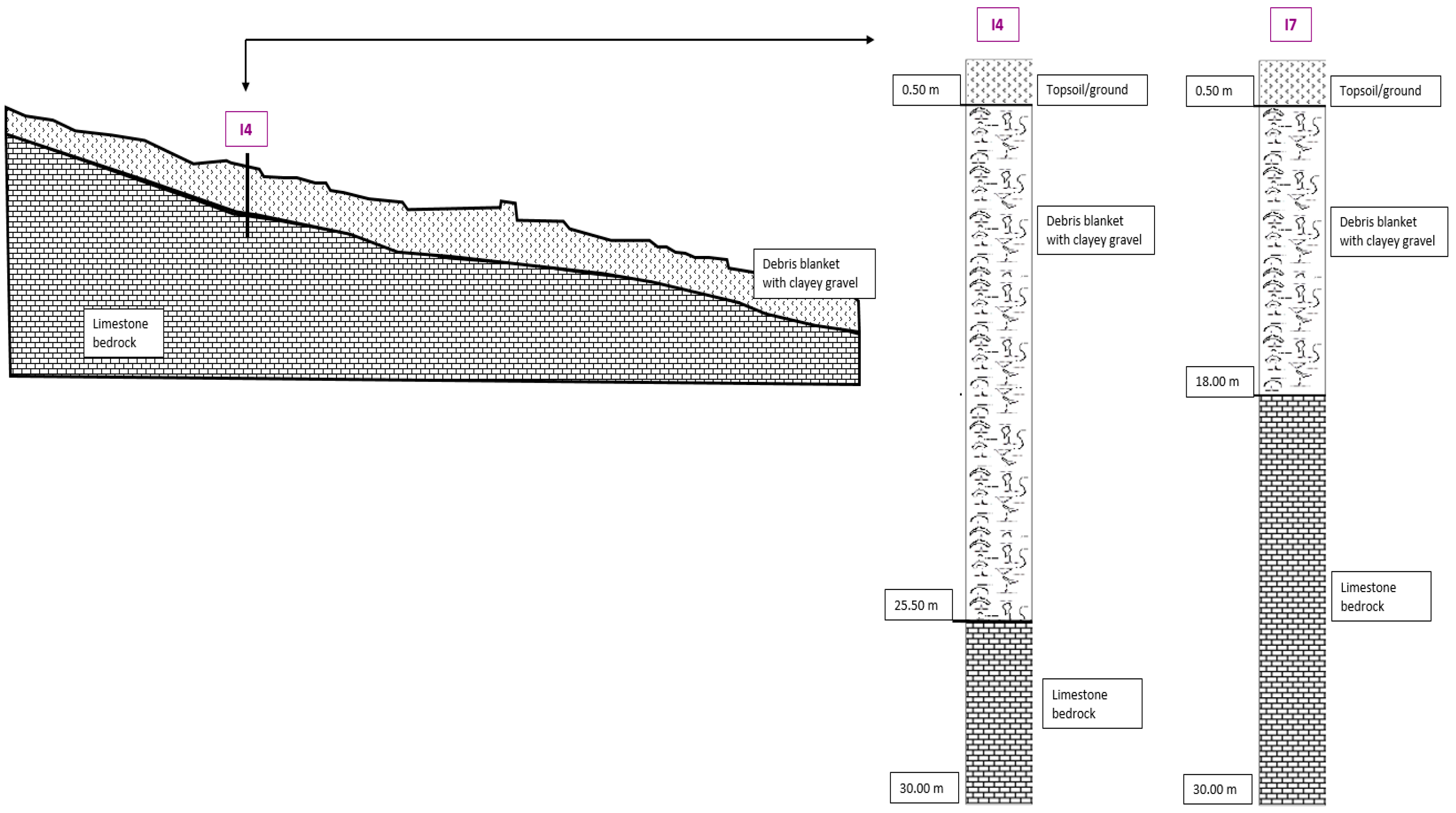
Figure 4 represents the simplified stratigraphy profile of the slope and the boreholes at I4 and I7. For brevity, the other boreholes are not presented, but even at I1, I2, I3, I5 and I8 (Figure 3) the subsoil can be assimilated into two layers: a debris blanket (clayey gravel), whose thickness ranges between about 10–25 m, and an underlying bedrock (limestone).

Light SPTs were also performed at two points (red dots in Figure 3), in order to determine the value of the friction angle, φ′. From the elaboration of these tests, the values of φ′ pertinent to the upper 5 m of soil are between 28° and 30°.

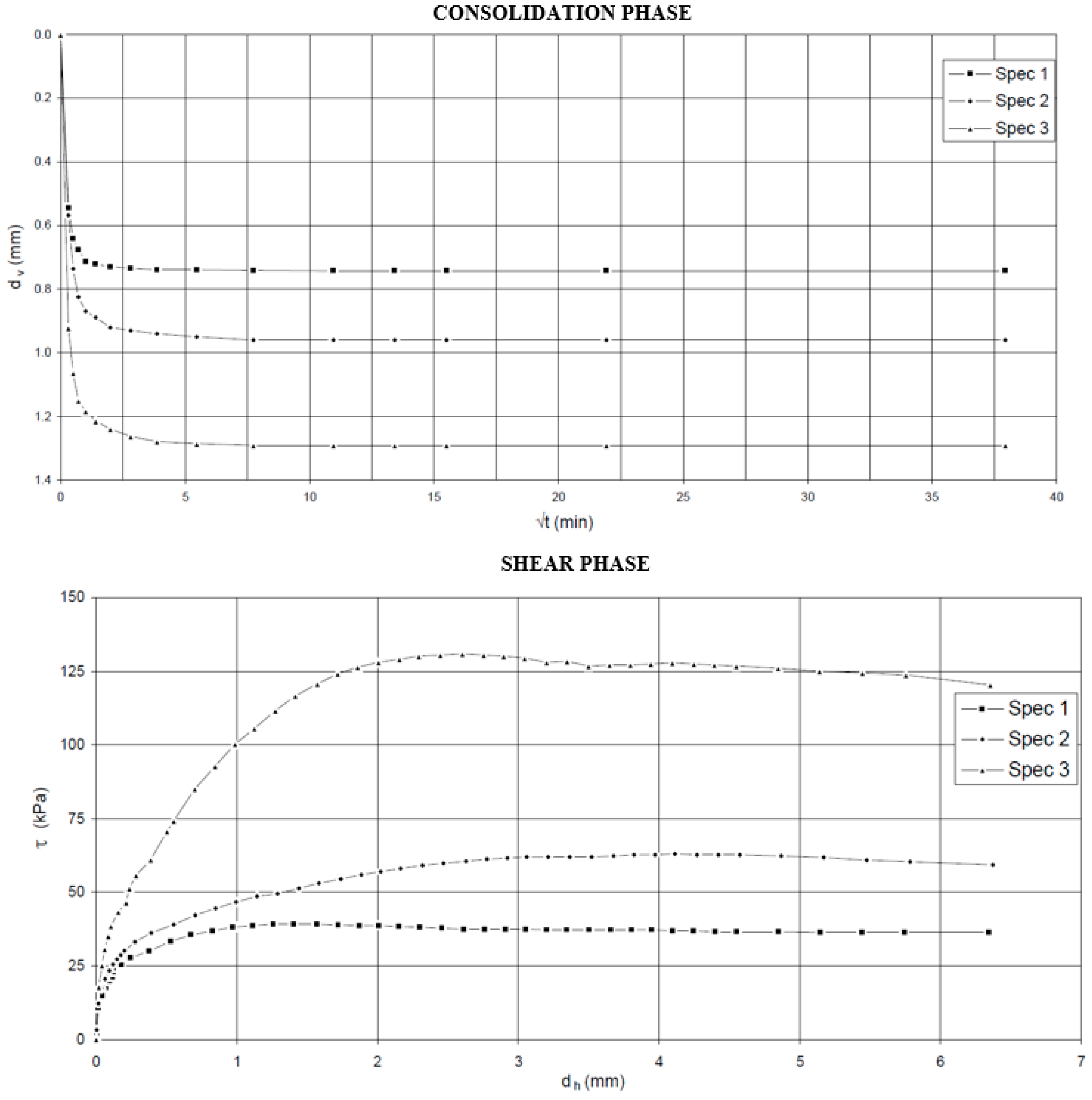
Only one direct shear test on three undisturbed specimens was performed (

Table 1. Direct shear test and specimens details.

		Specimen 1	Specimen 2	Specimen 3
H [cm]	Specimen height	2.31	2.31	2.31
D [cm]	Specimen diameter	6.00	6.00	6.00
Velocity [mm/min]	Applied shear velocity	0.005	0.005	0.005
σv [kPa]	Vertical stress	50.00	100.00	200.00
ΔHc [mm]	Vertical consolidation shortening	0.74	0.96	1.29
ΔHf [mm]	Vertical failure shortening	0.07	0.16	0.22
dh [mm]	Horizontal failure displacement	1.26	4.11	2.60
τf [kPa]	Failure shear stress	39.20	63.00	130.70

). A thin walled Shelby tube was adopted for sampling at depth between 3 and 3.5 m. In Figure 5, the graphs of consolidation and shear phases are represented. A cohesion (c′) equal to around 5 kPa and φ′ equal to around 32° are evaluated by this test.

2.1.3. Geophysical Surveys

Geophysical surveys are indirect, non-invasive tests allowing the definition of a subsoil model. They are often used to characterize landslide bodies even of considerable size [22].

In August 2019, geophysical field surveys were performed at Ville San Pietro (Figure 3) in order to have more information about the site soils with moderate costs. In this occasion, three spectral analyses of microtremor recording [23] were performed in the lower part of the village (more precisely at A, B and C in Figure 3). This methodology represents a straightforward technique to evaluate local site effects and natural resonance frequency of a site by calculating the spectral ratio between the horizontal and the vertical component of the ground motion. For these analyses, a 24-bit triaxial digital seismometer by Sara Electronic Instruments was used. This instrument was connected to a computer, in order to immediately see the data acquisition. The seismometer records every vibration from 0.5 Hz: in this way, the natural microtremor could be recorded, but it is important to be sure of not having noises interferences from anthropic sources.

Two refraction tests were performed on the artificial dam, placed in the upper part of Ville San Pietro (at D in Figure 3). In this case, DoReMi geophones by Sara Electronic Instruments were used. In particular, sixteen geophones were installed in the ground at 2 m from each other. A circular metal plate was hit with a hammer 4 kg weight. Again, the connection of the geophones to a computer allowed the data acquisition in real time.

The data collected from the tests were processed to obtain the primary and secondary wave velocities (V_P and V_S, respectively). The geophysical investigations confirmed the presence of two layers: the blanket (the shallow layer characterized by a low primary wave velocity V_P = 378 m/s) and the bedrock (the deep rock layer characterized by high primary wave velocity V_P = 832 m/s).

2.1.4. Monitoring by Inclinometers and Piezometers

Ville San Pietro is monitored by piezometers and inclinometers, installed since 2008, to detect both water table fluctuations and soil displacements (Figure 3).

In the present study, the piezometer and inclinometer data, provided by the Regional Agency for the Protection of the Ligurian Environment (Agenzia Regionale per la Protezione dell’Ambiente Ligure-ARPAL), are analyzed. All the piezometer measurements have been performed by technicians using galvanometric probes. At the end of 2017, only the piezometer P3 has been equipped with an automatic galvanometric probe (OTR probe). All the inclinometer measurements have been executed by technicians adopting a biaxial servo accelerometer probe S060314.

The first measures date back to the end of 2009. From that moment, piezometer and inclinometer measurements should have been carried out at a frequency of 6 months, namely two readings every year. However, this frequency was not respected: in fact, as shown in Figure 6, some years have been poorly monitored. Only in the last few years have the measurements been increased (sometimes three or four every year), thanks to the European AD-VITAM project. The lack of data in the past few years is a problem for a proper observation of the slope behavior.

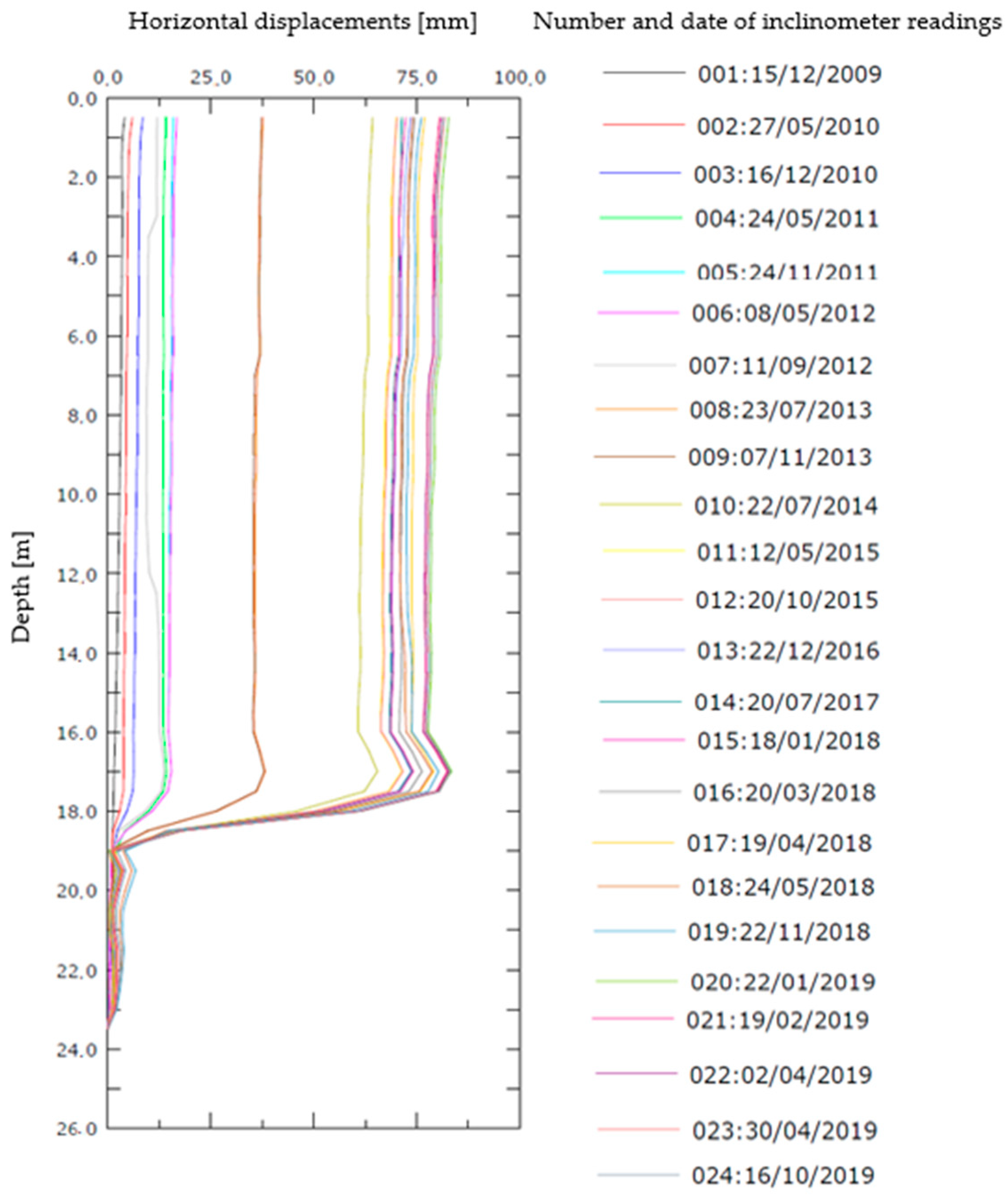
All the inclinometers detect the transition from stable to unstable layer at depths around 14–20 m. Moreover, the inclinometer curves are almost constant (with a gradient of about 2 mm per meter of depth) in the blanket (Figure 6). Hence, a prevalent translational sliding occurs. Unfortunately, the displacements induced the failure of two inclinometers. In fact, I5 and I1 went out of order in 2013 and in early 2018, respectively.

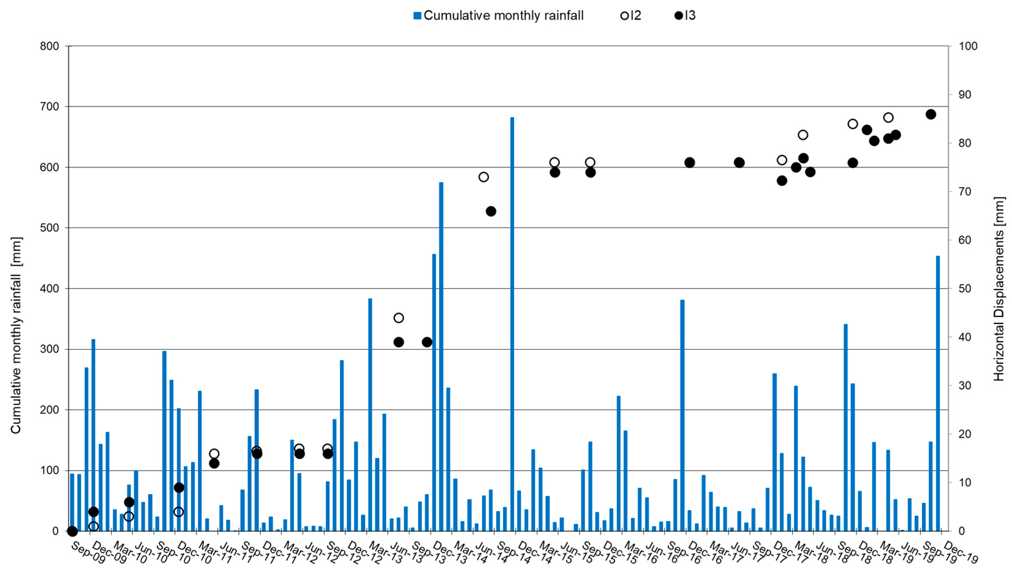
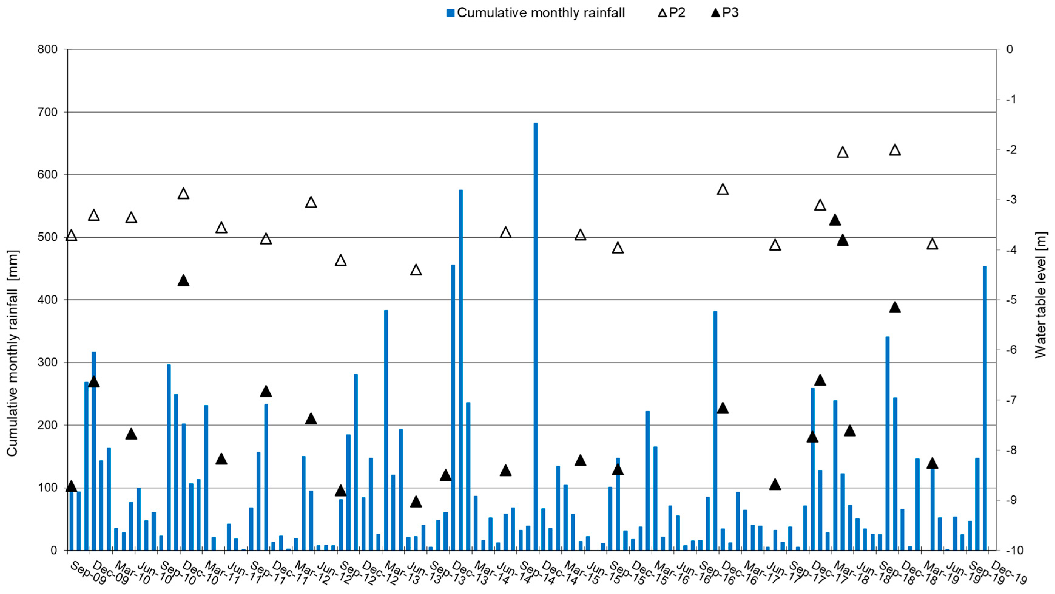
It is interesting to observe the diagrams of soil displacement, water table fluctuation and cumulative monthly rainfall. In Figure 7, the cumulative monthly rainfall and the ground displacements at the head of the inclinometer I2 and I3 are shown, while Figure 8 shows the cumulative monthly rainfall and the water table fluctuations, recorded by the piezometer P2 and P3 during the months between September 2009 and December 2019.

Unfortunately, the failure of the inclinometer I5 and I1 and the time lapse between the inclinometer and piezometer readings, do not allow an appropriate analysis of the slope behavior over time. The information from piezometers and inclinometers (Figure 7 and Figure 8) do not show a clear relationship between the water table fluctuations and the ground displacements, while the occurred ground movements are in accordance to the observed rainfalls.

The further measurements that will be provided and the water content measurements that will be carried out by the LAMP WSN will allow to deepen the hydraulic and mechanical behavior of the slope. It is worth pointing out that when installing the networks of the LAMP system, soil samples are taken at the nodes. The laboratory analyses conducted on the material collected will be useful to better characterize the shallow soil layer (within the first meter), especially from the hydrological point of view, to better study the infiltration of rainwater into the soil.

2.1.5. SAR Interferometry Monitoring

The slope monitoring techniques include traditional topography, the use of satellites and Global Navigation Satellite System (GNSS), photogrammetric techniques, 3D laser scanner and Synthetic Aperture Radar (SAR).

The SAR data has been adopted in order to have further information about the slope movements in Ville San Pietro. The use of this technique for land planning and management is recent and in fast developing [24]. Unfortunately, the SAR technique is barely known and therefore still rarely exploited by technicians.

In particular, the technique called PSInSAR (Persistent Scatterer Interferometric Synthetic Aperture Radar) was used during the Interreg IIIa Alcotra RiskNat project. This project was aimed at the study and control of landslide movements by the use of radar-interferometry techniques. The PSinSAR technique allows evaluating the velocity of targets in the ground over time, with a precision of 1 mm/year. The targets, called Permanent Scatterers (PS), could be both natural elements, for example rocks or areas free of vegetation, and anthropic as buildings, streetlights or metal structures that could reflect the radar signal. The PSinSAR technique is based on a comparison of series of radar images at different times, in order to evaluate the velocities of the targets. The advantages of this technique are the possibility of investigating extended areas in a rather short time and at low cost, because often the targets are already on the site and they have not to be installed. Where their density is high, an optimum identification and characterization of slow landslides is achieved. The satellites can measure only one component of the landslide movement because of the geometry of their orbits; this fact is related with the concept of “line of sight” (LOS) between the satellite and the target. This can result in an underestimation of the landslide displacement. Hence, the LOS velocity is generally projected along the slope [25].

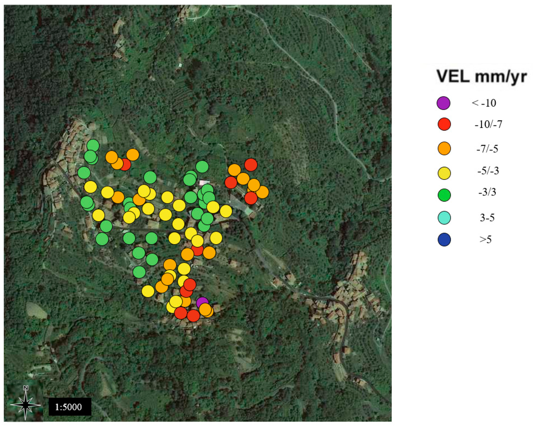
In Ville San Pietro, 23 PSs were identified, but only 19 are significant. These are in the built-up area (Figure 9).

2.2. Three-Dimensional Finite Element Modeling of Ville San Pietro

The three-dimensional numerical analyses reported in this paper are performed by means of PLAXIS 3D, property of Bentley Systems, in order to study the slope behavior and define the location of the monitoring network nodes. PLAXIS 3D is a full three-dimensional finite element code, used for geotechnical engineering and design.

Data of rain, groundwater levels and soil displacements, provided since 2009, when Ville San Pietro monitoring began, have been used. In particular, a well-documented period (January 2018–March 2018) was considered for the model calibration. Moreover, the groundwater level fall, occurred between March 2018 and June 2018, was simulated for the model validation. These periods have been chosen because of the good frequency of measurement and consequently for the considerable amount of available data, as shown in Figure 7 and Figure 8.

When the LAMP monitoring network will be in operation, new data will be available. The water content measurements will be used for a proper characterization of the shallow soil layer and soil unsaturated conditions will be properly taken into account. As the WSN will be active, the Ville San Pietro numerical model will allow to make useful comparisons with what will be obtained by the application of the IHG model implemented in the LAMP system.

It is worth underlining that taking into account the unsaturated soil is particularly important when the kinematic phenomenon concerns shallow soil layers. Rainfalls can cause a reduction in matric suction near the ground surface due to water infiltration. Such a phenomenon can be the triggering factor for shallow landslides, especially for fine-grained soils. In the case of Ville San Pietro, the inclinometers highlight almost constant displacements in the blanket (made up of clayey gravel) up to a significant depth, ranging between 14 and 20 m, and the main water table is at depths between 3 and 8 m from the ground level (e.g., the water table levels observed by P2 and P3 are reported in Figure 8). Therefore, it was decided (not yet having an appropriate characterization of the soil and the monitoring of the water content by means of the LAMP network) to neglect the behavior of the soil in unsaturated conditions and to simulate the oscillations of the groundwater, measured by piezometers. The displacements obtained from the numerical analyses are then compared with the displacement measurements carried out by the inclinometers on occasions of the studied groundwater fluctuations.

Hence, the current FEM analyses simulate the response of the slope in the event of water table oscillations by Plastic phases. In particular, for the selection of the soil parameter the water table fluctuations are simulated, and the computed displacements are compared with the real detected ones by inclinometers. Safety analyses follow the Plastic phases.

In order to validate the model, the critical areas identified by the numerical code are confronted with the areas actually subject to displacements (detected by inclinometer and interferometry monitoring data) and affected by damages (observed by on-site inspection).

2.2.1. Governing Equations

In the present research, each simulation by PLAXIS 3D consists of several phases. The Initial Phase is calculated by the Gravity Loading technique. A raising or lowering of the water table is simulated by means of two Plastic phases, relating to the initial and final level measured by the piezometers. The fluctuations in the groundwater level are simulated regardless of their variation over time. Water flows in the soil and unsaturated conditions are not considered. Hence, pore water pressures are not time dependent, the hydro-mechanical problem is not coupled and Terzaghi’s law can be adopted for the calculation of the soil effective stresses. As far as the stress–strain relationships are concerned, it is investigated whether to use the Linear Elastic, Perfectly Plastic Model (i.e., Mohr–Coulomb model) or the Hardening Soil model.

On the basis of a soil stress–strain analysis, the study of the slope behavior in case of water table fluctuations is studied and the slope stability conditions are evaluated by Safety analyses (following the Plastic phases) which are global stability analyses conducted by the Shear-Strength Reduction Technique (SSRT) [26]. The Safety analysis provides the failure mechanism and the pertinent Safety Factor. As well known, the Safety Factor (SF) evaluates the stability degree of the slope. It is important to underline that the displacements evaluated by a Safety analysis are not realistic. In fact, in the implementation of the Shear-Strength Reduction Technique in Mohr–Coulomb model, the magnitude of some nodes’ displacements become abruptly large as the slope failure is reached. Generally, the SSRT gives similar safety factors as obtained from conventional stability analyses based on the Limit Equilibrium Method (LEM) [27].

2.2.2. Slope Model Geometry and Discretization

As far as geometry is concerned, according to the boreholes, the stratigraphy is composed of two layers: a debris blanket and a bedrock.

For modelling the stratigraphy, the two surfaces representing the upper and lower limits of the blanket have to be introduced. The former is deduced from the Digital Terrain Model (DTM); the latter is obtained by interpolation, in GIS environment, of the data obtained by the surveys described in the previous sections. The model volume is created with the geometry processing in PLAXIS 3D.

The mesh is composed by 10-node tetrahedrons. In consideration of the size of the model and for limiting the calculation time, a Medium mesh with a major density for the blanket (Coarseness Factor = 0.5) is chosen. The model is composed of 56,780 soil elements with 85,134 nodes.

Several groundwater surfaces are created by interpolation in GIS environment of the data obtained by the piezometer measurements. Above the water table the soil is assumed to be dry, while below it is saturated. The mechanical boundary conditions on the lateral and base surfaces are imposed as “Fully Fixed”, in order to simulate the confinement effect of the external soil. The hydraulic boundary conditions pertinent to the same surfaces are “Closed”, to prevent water flow through the boundaries.

The properties of the blanket and the bedrock are calibrated on the basis of the geotechnical and geophysical surveys. The parameters are properly chosen so that the model simulates the actual behavior of the slope. The model parameters and calibration are reported in the following sections.

2.2.3. Church Modeling

In order to create a more realistic model of the slope, numerical analyses should be carried out considering the buildings located on the slope.

The church is the structure to be included as a priority, since it is the most significant building from the historical and cultural point of view, the most damaged and certainly, the most considerable with reference to the load applied to the ground. In fact, the church, dating back to 1776, is the most imposing building in Ville San Pietro. It is located in an area subject to displacements, measured by the inclinometers located nearby (Figure 10a), and it shows evident damages (Figure 10b).

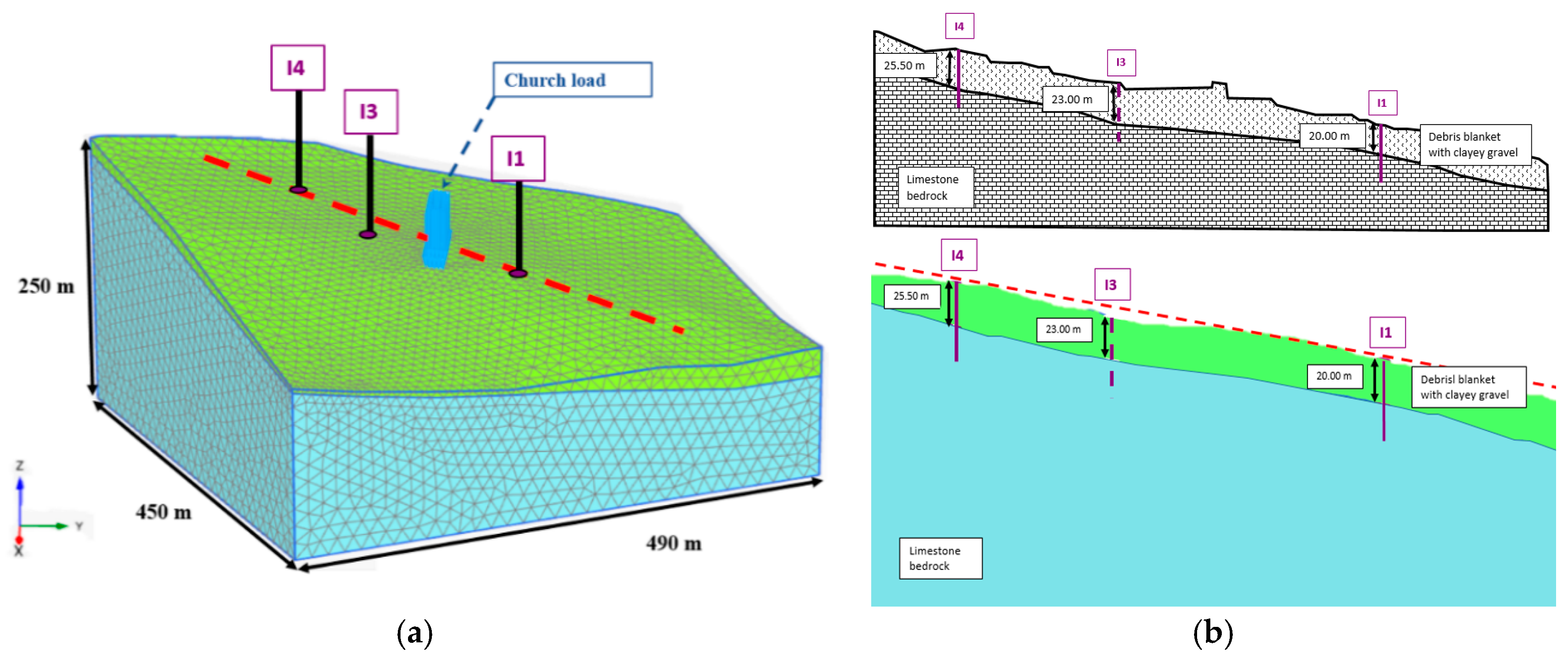
For operational reasons, the church is inserted in the present 3D slope model in a simplified way. More precisely, the load this building applies to the ground is modelled, regardless of the real soil-structure interaction. The load per unit area of the church is inserted in the model on a rectangular surface, containing the actual base section. This area is previously defined in GIS environment and then imported into PLAXIS 3D. Using the Digital Surface Model (DSM) and the observations during the inspection, an average height of the building of about 15 m is obtained, but to be more punitive, a higher value equal to 17 m is fixed. The plant is assumed to be 27 m × 15 m. As no detailed information are available, especially regarding the structural characteristics, the church load is assessed in a simplified way. In particular, the perimeter walls, estimated 50 cm thick, are assumed to be composed of stone and mortar. By viewing the images, it is found that the church roof is composed of tiles.

Furthermore, the presence of a 50 cm high limestone foundation slab and the presence of a 10 cm high marble floor are assumed. Using the values indicated in

Table 2. Volume Unit Weight and Surface Unit Weight adopted for the evaluation of the church load.

Materials [-]	Volume Unit Weight [kN/m3]	Materials [-]	Surface Unit Weight [kN/m2]
Concrete	24	Tiles	0.80
Slate	27
Limestone	26
Marble	27
Stone and mortar wall	22

, a load pressure equal to 55 kPa is evaluated. Therefore, this pressure is applied to the 3D slope model in order to take the church into account (Figure 11). In Figure 11a, the final model of the slope is presented. It consists of two layer (i.e., the blanket and the bedrock) and the load of the church is applied to the ground. As shown in Figure 11b, the cross-section, passing through most of the inclinometers (indicated by purple lines), is investigated. There is a good accordance between the detected stratigraphy profile and the numerical model cross-section.

2.2.4. Slope Model Parameters

After the definition of the geometry in PLAXIS 3D, the following step is to assign proper values to the soil properties. In the first instance, it was established to characterize both layers by the Mohr–Coulomb constitutive model (synthetically denoted as MC in the following). The Linear Elastic, Perfectly Plastic Model (MC) simplifies the actual soil behavior. Even if it is well known that an accurate assessment of soil displacements requires the adoption of non-linear constitutive laws (able to describe the stiffness dependence on the stress and strain), the Mohr–Coulomb model is widely used in geotechnical modelling. It is particularly convenient when laboratory tests are scarce, as in the case of Ville San Pietro. In fact, it requires only two stiffness parameters. The input parameters are the soil unit weight γ, the effective cohesion c′, the friction angle φ′, the Poisson’s coefficient v and, the shear stiffness modulus G (or, alternatively, the Young’s modulus E). The data obtained from the laboratory tests are used for fixing the unit weight values of dry and saturated soil (γ_dry, γ_sat, respectively), pertinent to each layer; these values are also confirmed by the geophysical test results.

For the determination of the most suitable strength parameters of the blanket, preliminary numerical analyses were conducted. They are not reported in this paper for brevity, but they are only briefly described. First of all, global limit equilibrium analyses were performed. The blanket was characterized by the γ_dry and γ_sat values reported in

Table 3. SET MC.

Soil Properties	Blanket	Bedrock
${\gamma }_{dry}$ [kN/m3]	18	27
${\gamma }_{sat}$ [kN/m3]	21	30
φ′ [°]	28	35
c′ [kPa]	8	10
v [-]	0.30	0.30
E [kPa]	107,339	4,953,530
G [kPa]	41,284	1,905,204
$K_0$ [-]	0.43	0.43

, while c′ was assumed equal to 0 kPa and φ′ equal to 22°, which are the most punitive values from the test result elaborations. These analyses were conducted on three significant cross-sections of the slope with several water table levels and in all these cases the provided Safety Factors were less than one (about 0.5–0.7). These results were not coherent with the observed slope behavior. Therefore, additional preliminary finite element analyses (on the aforementioned slope cross-sections) were carried out increasing the above strength parameters, but always referring to the experimental test results. The adopted values of γ_dry, γ_sat, v and E are indicated in Table 3 (the estimate of the stiffness parameters is described below). In particular, characterizing the blanket with the values of cohesion and friction angle from the direct shear test, the analyses disagreed to the actual slope response.

Thereby, at the end of these parametric analyses, it was concluded that the most suitable strength parameters for the simulations were those presented in Table 3 and

Table 4. SET HS.

Soil Properties	Blanket	Bedrock
${\gamma }_{dry}$ [kN/m3]	18	27
${\gamma }_{sat}$ [kN/m3]	21	30
φ′ [°]	28	35
c′ [kPa]	8	10
v [-]	0.30	0.30
E [kPa]	---	4,953,530
G [kPa]	---	1,905,204
$E_{50}^{ref}$ [kPa]	40,000	---
$E_{oed}^{ref}$ [kPa]	20,000	---
$E_{ur}^{ref}$ [kPa]	120,000	---
m [-]	0.70	---
$K_0$ [-]	0.43	0.43

. The bedrock is characterized by strength parameters greater than those of the blanket, according to the geotechnical investigation.

For the evaluation of the stiffness parameters, the geotechnical and geophysical in situ tests are considered. Empirical correlations can be used for the estimates of the stiffness parameters [28]. Some of them provide directly the value of the shear stiffness modulus (G), others allow to calculate the secondary wave velocity (V_S) values and then, by the Equation (1) the value of the initial shear stiffness G₀

$$G_0=\frac{V_s^2\ast \gamma }{g}$$

(1)

where γ is the soil unit weight, g the gravitational acceleration.

In order to define the shear modulus of the blanket and the bedrock, a value of V_S = 150 m/s and 444 m/s is, respectively, used. Table 3 indicates the set of parameters adopted for the numerical simulations (K₀ is the coefficient of lateral earth pressure). The Mohr–Coulomb constitutive model is adopted for the blanket and the bedrock. The shear stiffness G is assumed equal to the initial value G₀.

Moreover, in order to investigate the appropriateness of an advanced constitutive model, the Hardening Soil (denoted as HS in the following) model is adopted for the blanket. Therefore, the simulations are repeated assuming the Hardening Soil model for the upper layer.

The advantage of the Hardening Soil model over the Mohr–Coulomb model is not only the use of a hyperbolic stress–strain curve instead of a bi-linear curve, but also the control of the stress level dependency. The HS model requires the following basic parameters for soil stiffness [29]:

• $E_{50}^{ref}$ reference stiffness modulus for primary loading, corresponding to the reference pressure
• $E_{ur}^{ref}$ reference Young’s modulus for unloading and reloading, corresponding to the reference pressure
• $E_{oed}^{ref}$ oedometer modulus, corresponding to the reference pressure
• m power for stress-level dependency of stiffness

where the reference pressure is generally assumed equal to 100 kPa.

Unfortunately, the lack of adequate laboratory tests does not allow the proper estimate of the stiffness parameters. In the present paper, they are fixed by Equations (2)–(4), assuming m = 0.70 [30].

The parameters belonging to the SET HS are indicated in Table 4.

$$E_0=E_{ur}^{ref}$$

(2)

$$E_{50}^{ref}=\frac{E_{ur}^{ref}}{3}$$

(3)

$$E_{oed}^{ref}=\frac{E_{50}^{ref}}{2}$$

(4)

As already mentioned, to select the model parameters, a series of analyses are performed with reference to the period between January 2018 and March 2018, simulating the water table rise, observed by the piezometers (e.g., Figure 8). The horizontal displacements measured by the inclinometers are compared with those calculated by the Plastic phases, simulating the water table oscillation, which actually occurs. Therefore, the initial condition is stated in January 2018 and all the measured displacements are from this date. Besides, all the measured displacements are referred to the bedrock, in which the inclinometer pipes are fixed. Analogous assumptions are made for representing the computed displacements, so that proper comparisons between simulated and measured displacements can be done.

The Safety analyses are adopted to ascertain if the numerical simulations capture the depth separating the portion of slope subject to displacements from the substantially stable zone below.

Any simulation in PLAXIS 3D consists of five phases. The Initial Phase is calculated by the Gravity Loading technique; the following two Plastic phases simulate the transition between the different groundwater levels firstly described. A Safety phase follows each Plastic one.

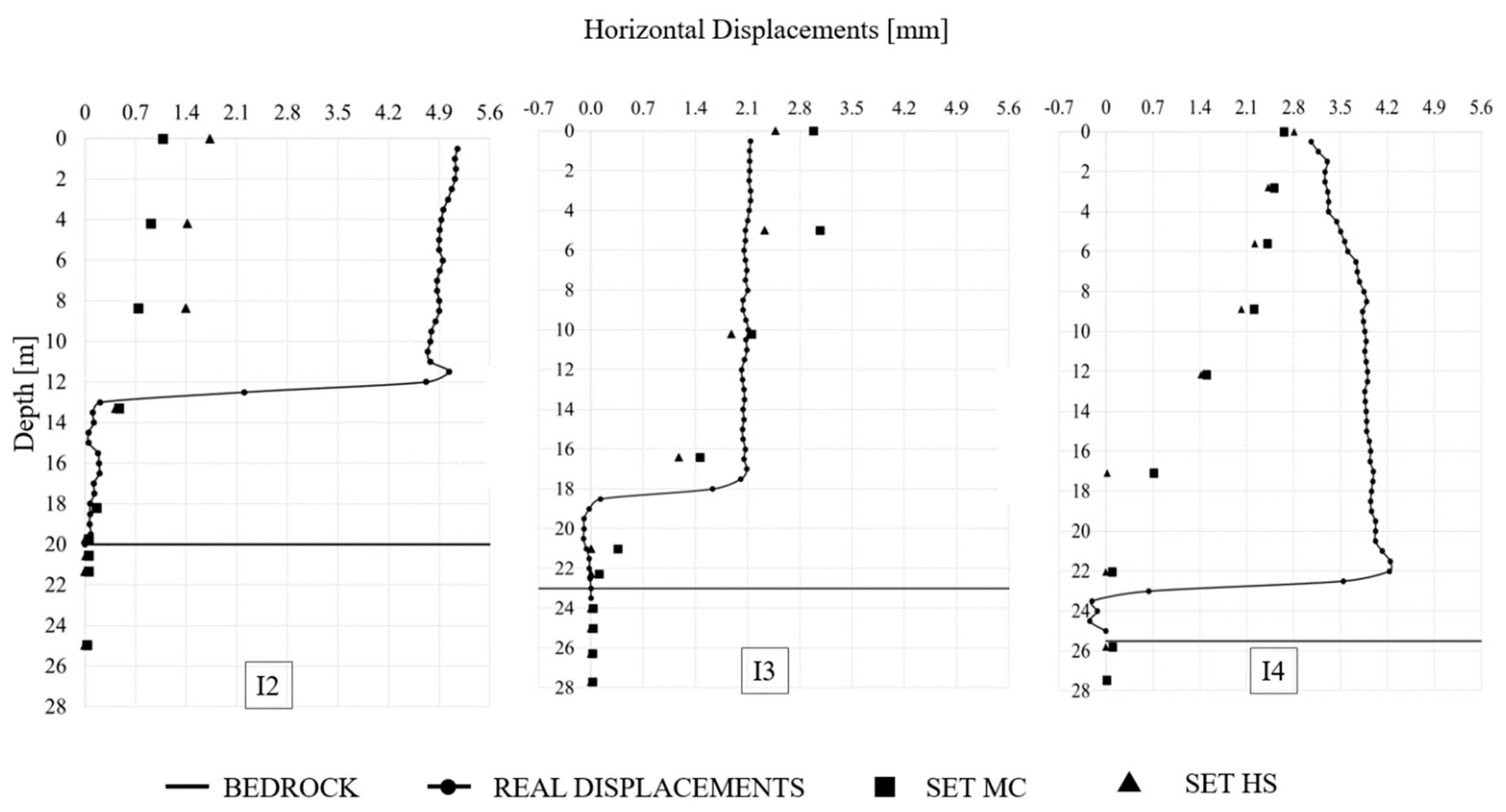
The most significant results, referred to the analyses conducted by using SET MC and SET HS, are reported in the present section. In particular, the horizontal displacements evaluated by PLAXIS 3D at the verticals, where the inclinometer I2, I3 and I4 are placed, are shown in Figure 12. In the phase representing the groundwater rise (occurred between January 2018 and March 2018), the horizontal displacements calculated at the I2 vertical underestimate the real values. For the same water table oscillation, at the I3 vertical, the Hardening Soil model allows capturing the trend of the inclinometer curve and the measured displacement values. However, with reference to the I4 vertical, the SET MC is slightly more representative of the real behavior. Additionally, at the vertical I2 and I4, the Hardening Soil model allows capturing the discontinuities of the inclinometer curves quite well.

The performed numerical analysis show that the Hardening Soil model seems more suitable to represent the behavior of the blanket. Consequently, the parameters of SET HS are assumed for the 3D slope model; in particular, the Hardening Soil model is adequate to represent the blanket behavior and the Mohr–Coulomb model is assumed for the bedrock.

3. Results

As above specified, five calculation phases (one Initial Phase and two Plastic phases, each followed by a Safety one) are performed by the model presented in the previous section. In the following, the numerical analysis results are shown. The model is validated by means of inclinometer tests, on-site inspections and SAR interferometry data.

3.1. Results of the Numerical Analysis Simulating the Groundwater Rise Occurred in January 2018–March 2018

In the following, with reference to the water table rise occurred between January 2018 and March 2018, the results of the Safety analysis are presented.

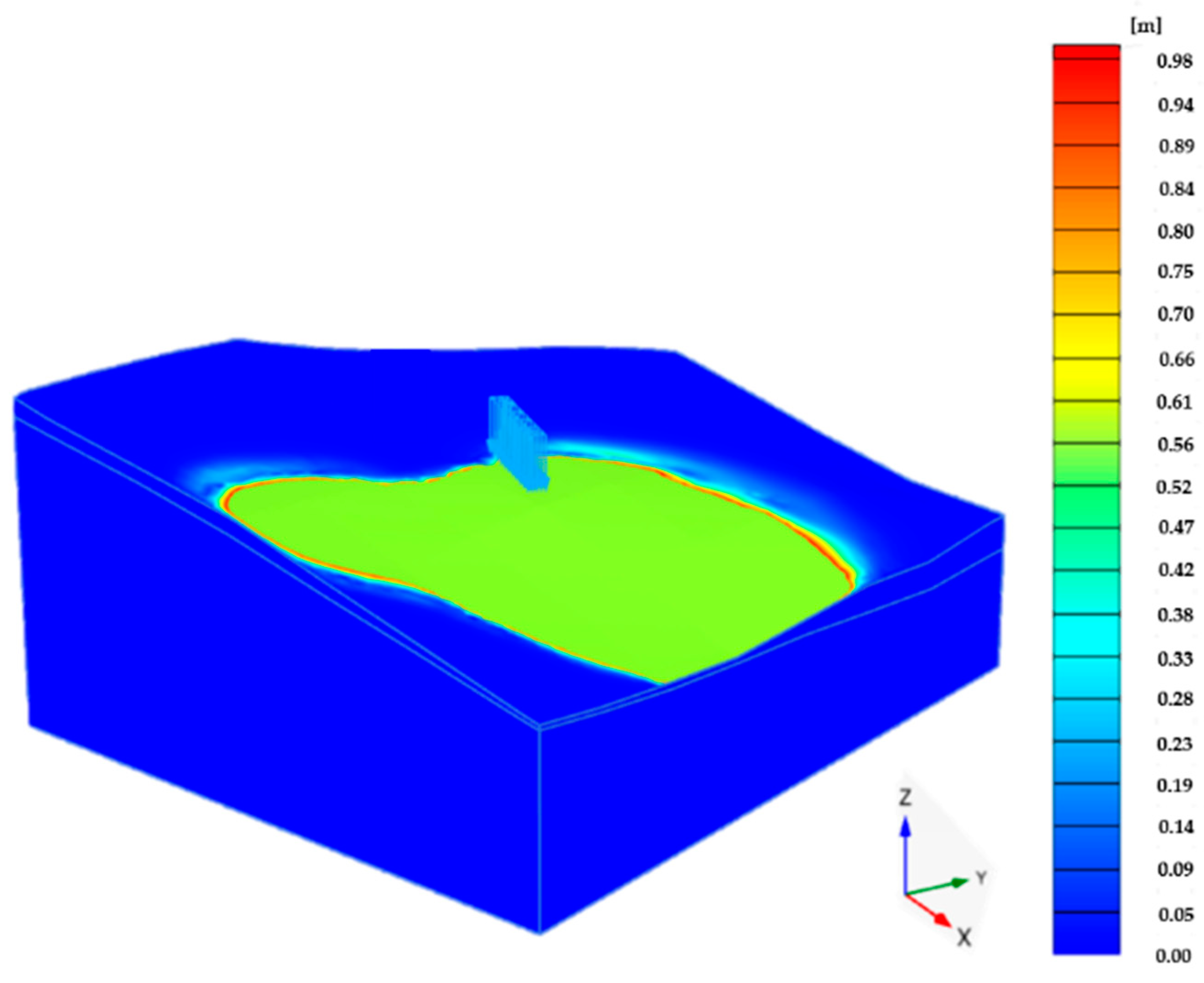
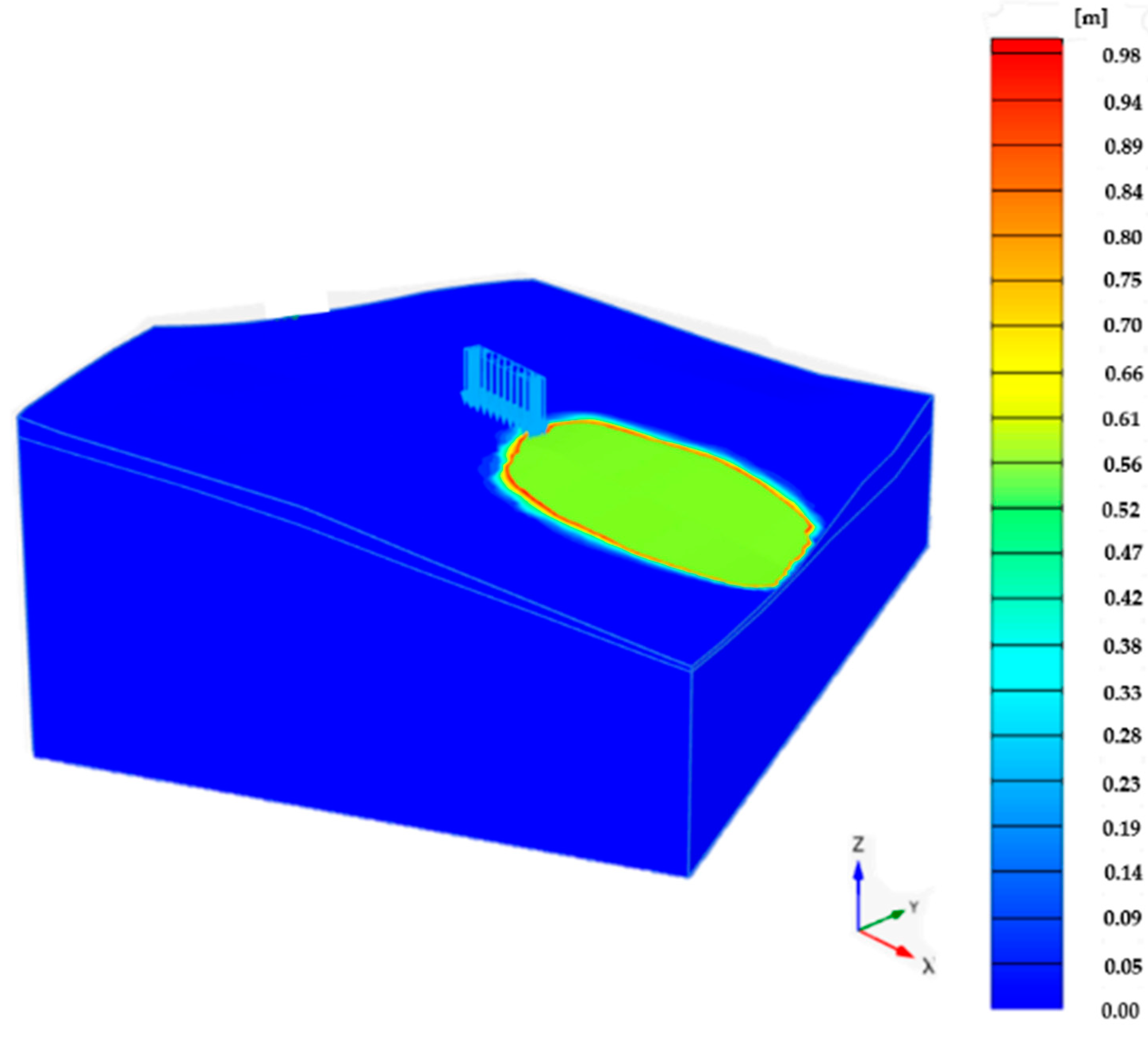
After the groundwater level rise, the Safety Factor evaluated by PLAXIS 3D is equal to 1.279. In Figure 13, the critical area, resulting from the numerical analysis, is quite extensive; in fact, the zone subject to movements extends around the church. Once more, it is important to remember that the Safety analysis displacement values have no physical significance. In particular, with regard to the inclinometer I2, I3 and I4, the Safety analysis captures the position of the discontinuity between stable and unstable soil, interpretable with the formation of a shear band. 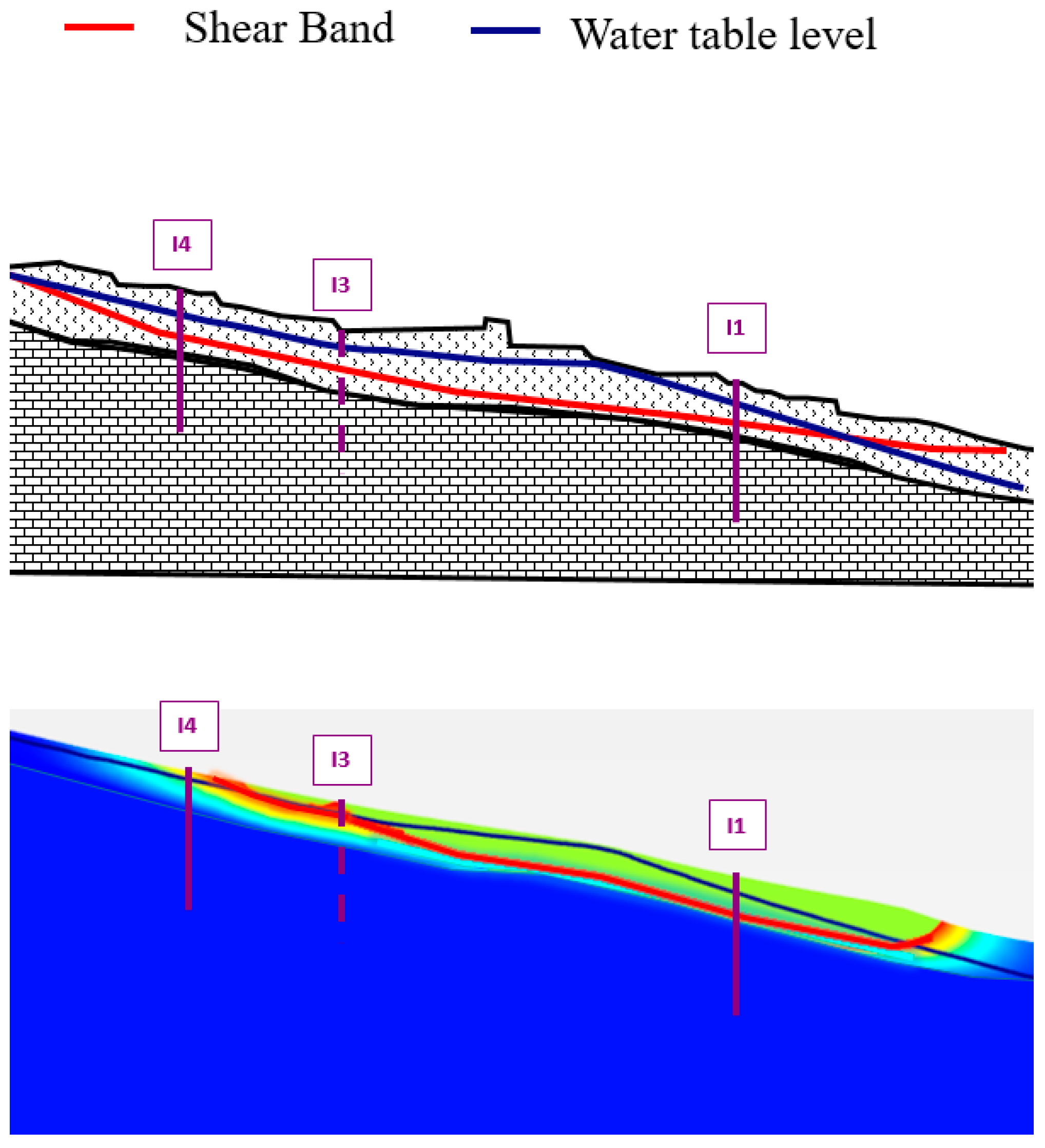Figure 14 shows the comparison between the shear band evaluated on basis of the tests performed by ARPAL and the PLAXIS one. As it can be seen, there is a good accordance in terms of critical areas.

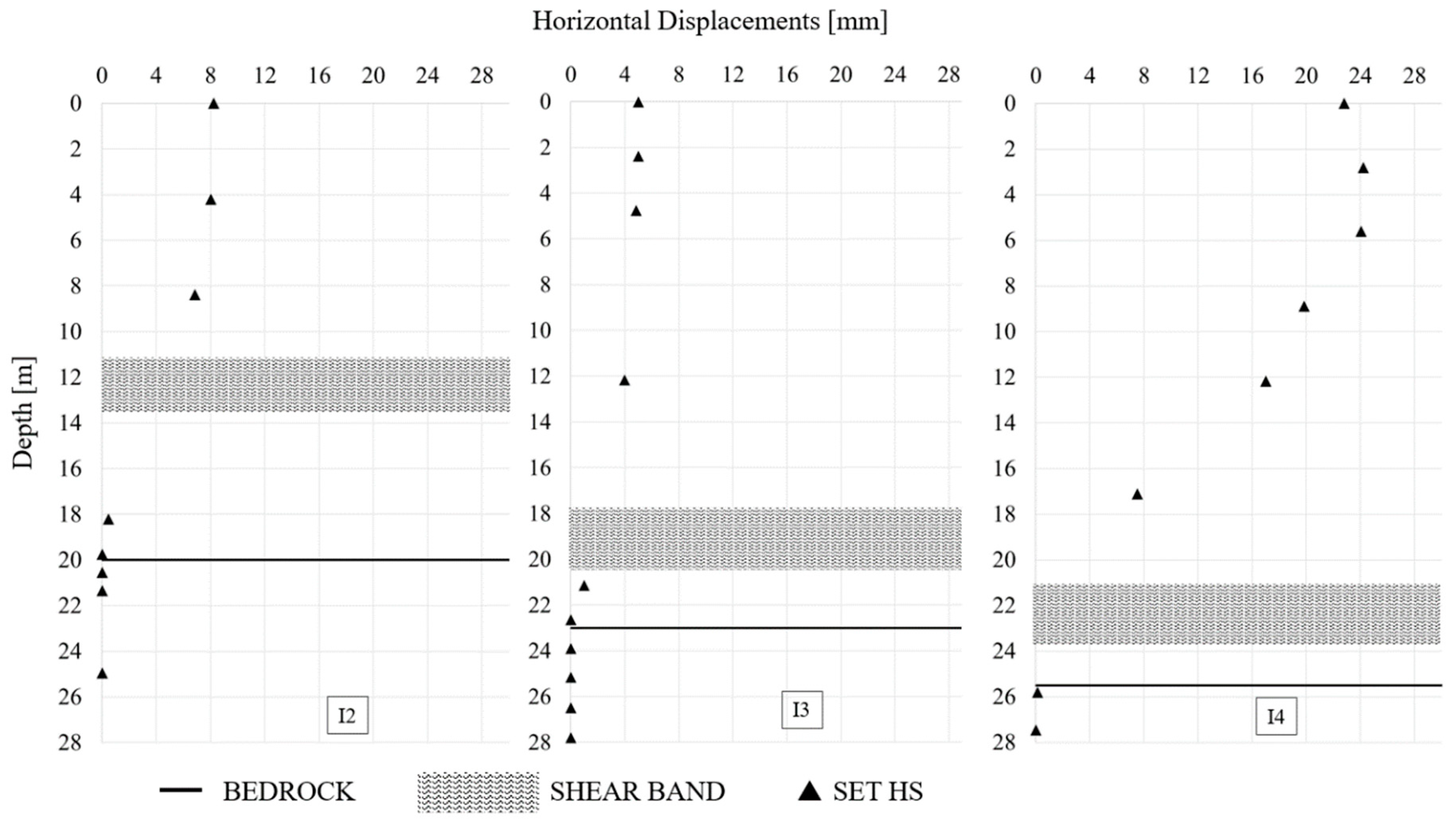
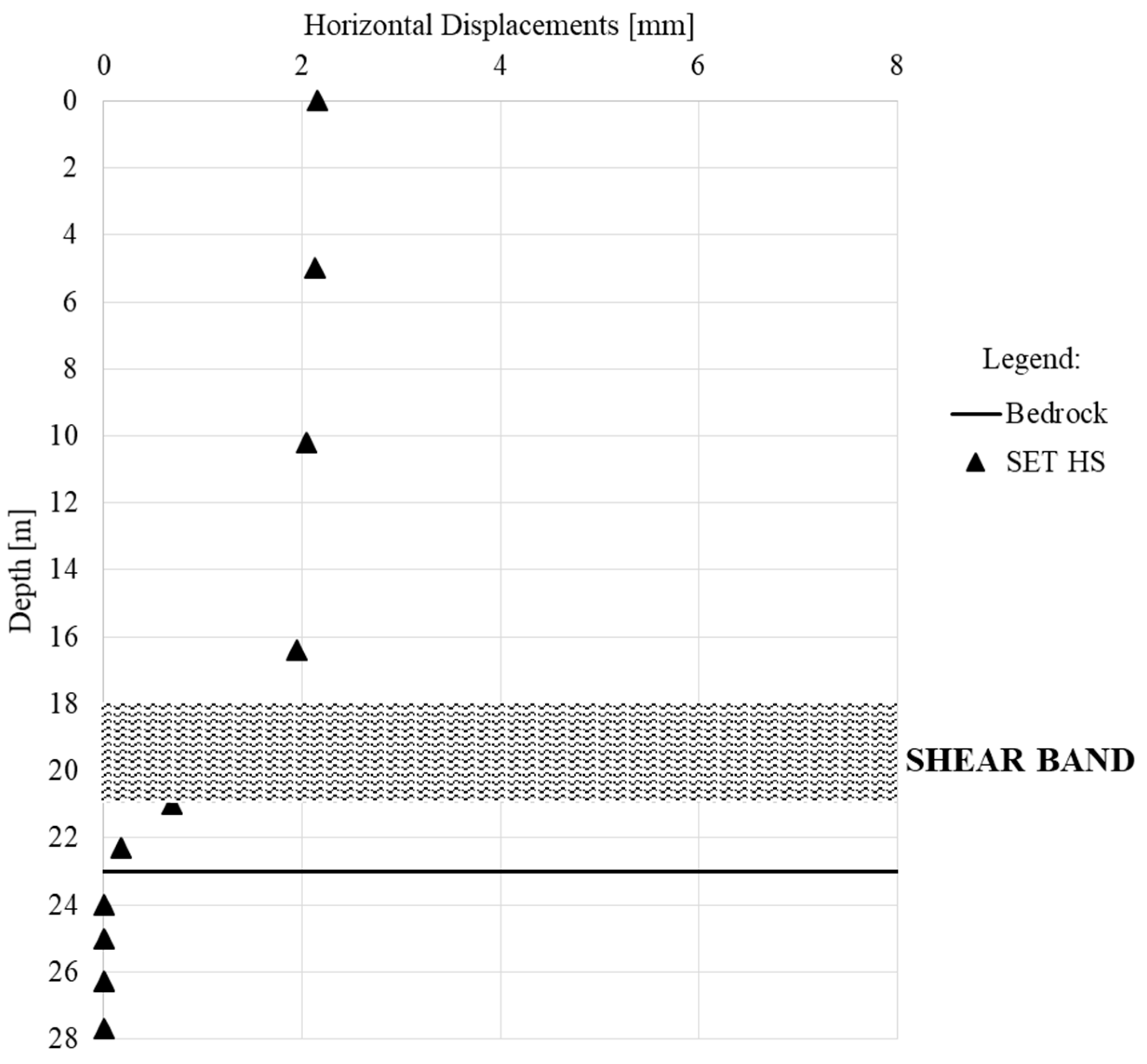
As shown in Figure 15, the position of the shear band is correctly represented by the Safety analysis: in fact, for I2, it is almost 13 m deep, i.e., it is close to the real one (between 11 and 13 m). Referring to the instrument I3: in this case, the Safety analysis distinctly represents the actual depth of the shear band (between 18 and 20 m deep). Similarly, for the inclinometer I4, the discontinuity between the stable layer and the unstable one is quite caught by the Safety analysis.

3.2. Results of the Numerical Analysis Simulating the Groundwater Fall Occurred in March 2018–June 2018

From March 2018 to June 2018, the water table dropped, as detected by the piezometers (e.g., Figure 7 and Figure 8). This water table fall is simulated by PLAXIS 3D, adopting the model described in the previous section. The computed displacements are compared with the real ones (Figure 16).

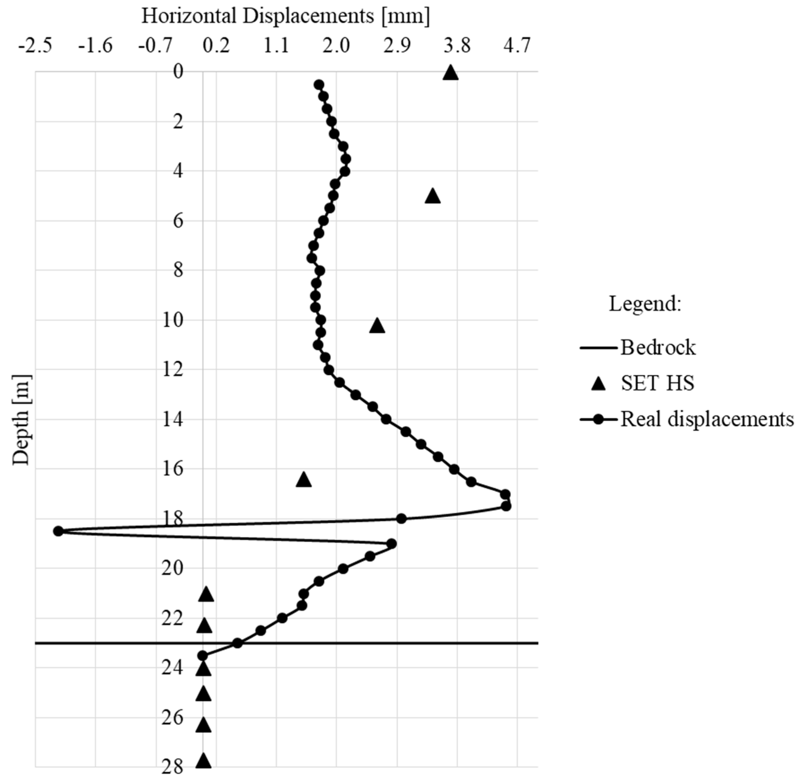
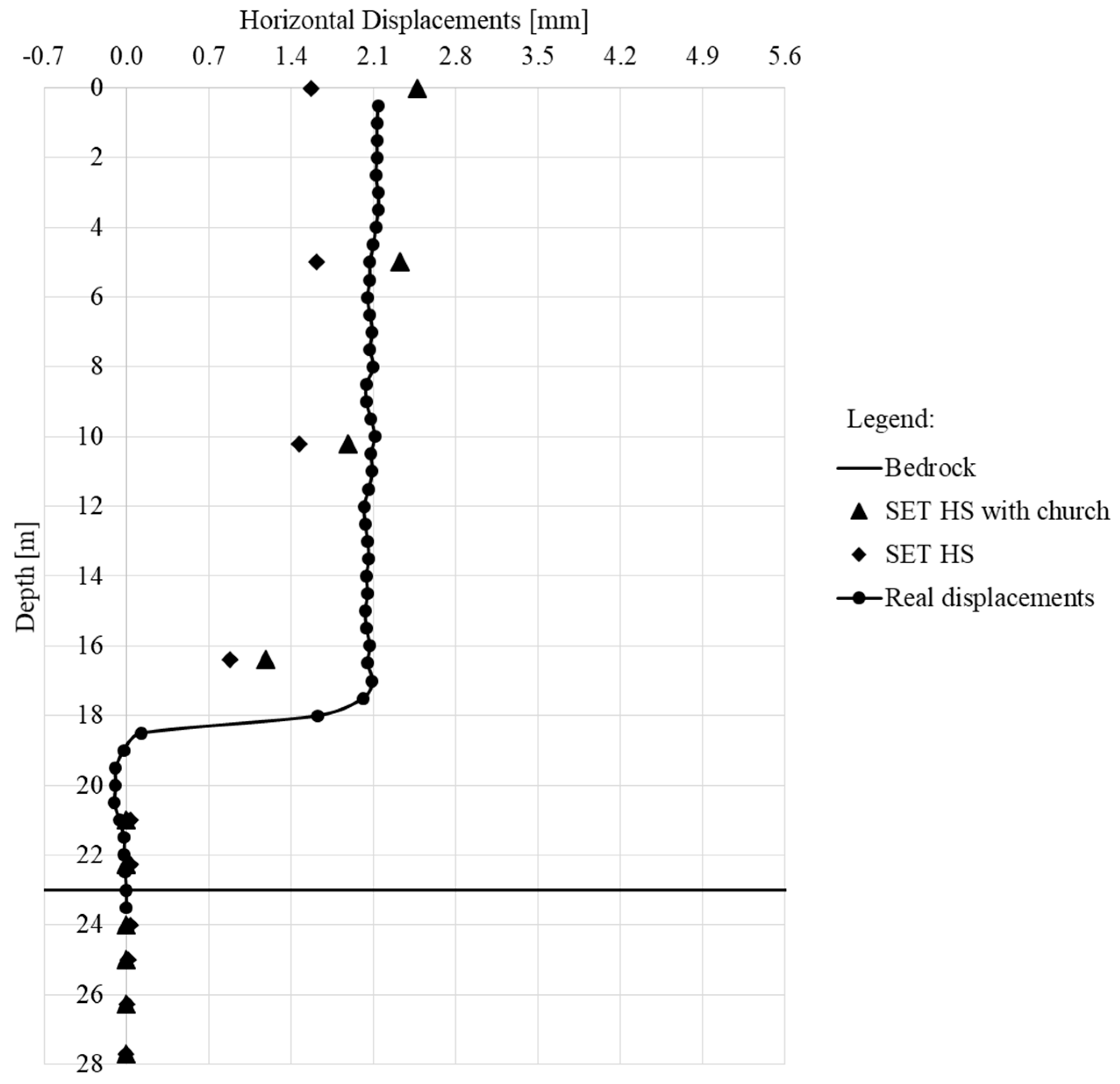
The presented results refer to the inclinometer I3, whose measurements are the only ones available in this period. As shown in Figure 16, the SET HS describes the behavior of the blanket that is close to the actual one, even in the case of a lowering of the groundwater.

In Figure 17 and Figure 18, the results of the Safety analysis are presented. After the groundwater level fall, the SF evaluated by PLAXIS 3D is equal to 1.357. In Figure 17, the critical area resulting from the numerical analysis is downstream the church.

With regard to I3 (Figure 18), the position of the discontinuity is correctly represented by the Safety analysis: in fact, it is between 18 and 21 m deep, i.e., it is close to the actual one (between 18 and 20 m).

After the lowering of the water table, as expected, the safety factor is greater than that obtained after the raising of the water table. In both cases it is greater than 1. This result is consistent with the actual conditions, since there is not an evident slope instability but the slope is subject to movements causing damages.

3.3. Numerical Analysis Results, On-Site Inspection and SAR Interferometry Data

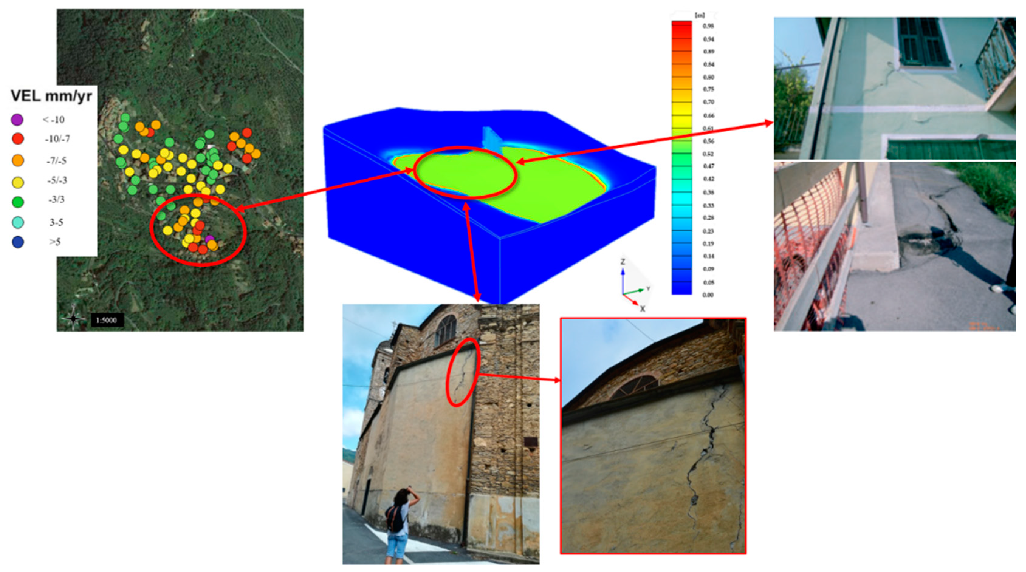
In the current section, the purpose is to check whether the areas that are critical from numerical modeling are actually problematic. In particular, the comparison is between the simulated critical areas, deduced by the Safety analysis after the groundwater level rise, and the real ones, observed during an on-site inspection and by means the PSinSAR technique.

During an inspection in Ville San Pietro, signs of damage were actually found in the critical areas of the model. In particular, damages to the structures and to the church, were evident (Figure 19).

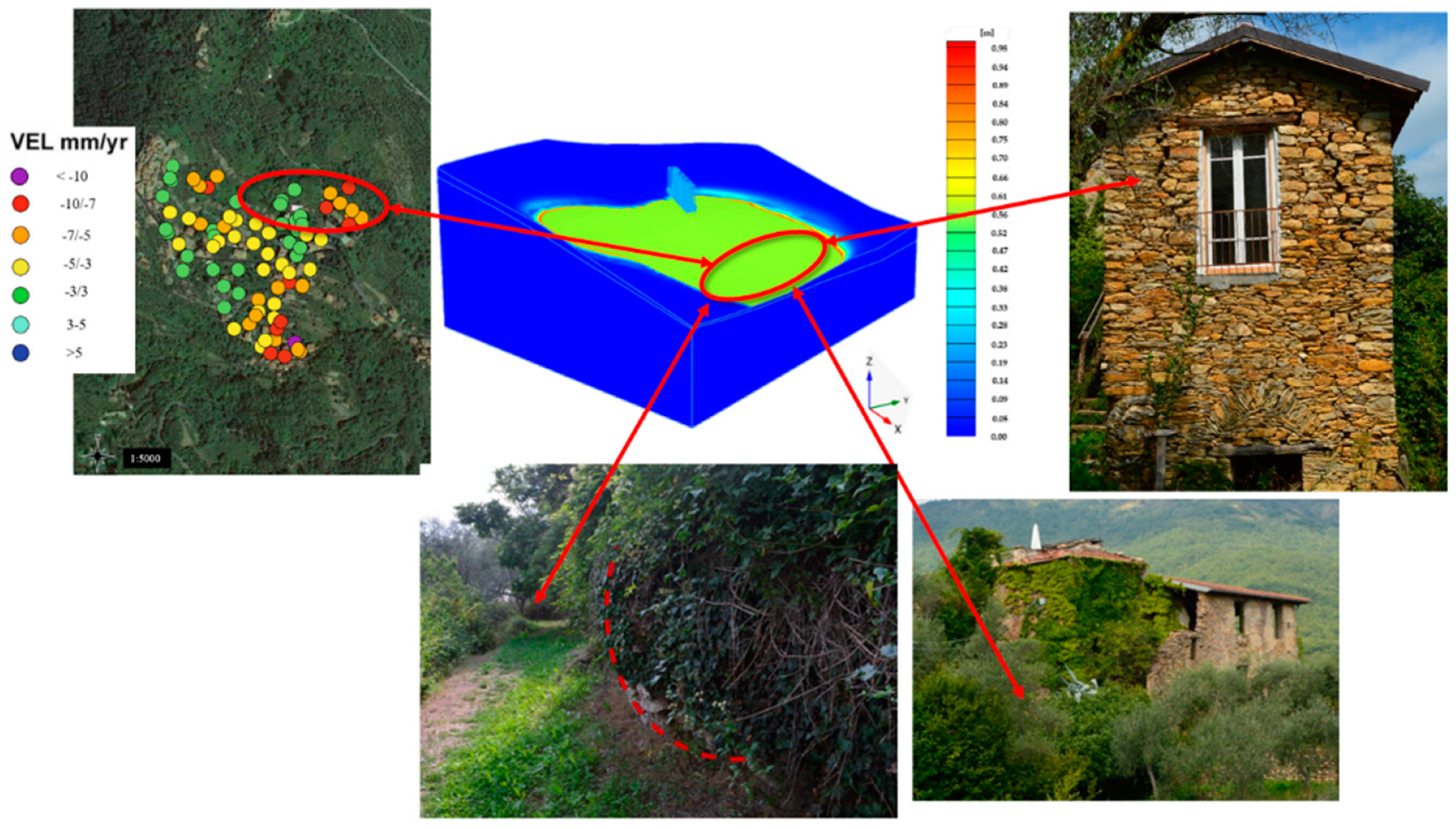
The PSInSAR technique detects significant slope movements at Case Soprane, which is located upstream of the church of Ville San Pietro, at the church itself and at the cemetery area. The PSInSAR technique identifies the lower part of the slope as an area subject to displacements (Figure 20). From the inspection, it is evident that this area is destined to agricultural and woodland use: the only evident signs of criticality are the marked deformations suffered by the retaining walls, which are present there.

In general, the results obtained by the numerical analysis are in good accordance with what can be noticed and measured in Ville San Pietro.

4. Discussion

In this paper, the first three-dimensional model of Ville San Pietro is described. This model is quite big. In fact, it represents a soil volume equal to 35.18 × 10⁶ m³. It is composed of a debris blanket and a stable bedrock and to better represent the real slope, the church load is introduced, albeit in a simplified way. For the usual purposes of geotechnical engineering analyses, this is quite uncommon, because the introduction of loads and the modelling of structures in 3D numerical models are onerous operations with regard to the determination of the geometry and material parameters, and the time consumption for calculation and output interpretation.

In Figure 21, the comparison between the results of the numerical analyses with and without the insertion of the church load is shown referring to I3, which is the inclinometer vertical closest to the church. As it can be seen, the insertion of the church load improves the simulation.

For a complete modelling, it would be necessary to insert all the buildings, although these are small and consequently their loads are modest. In this case, an accurate estimate of the pertinent loads applied to the ground would be necessary. Such an operation would be practicable, but onerous. Moreover, the interaction between soil and structures could be considered too, but the entire modelling would be very burdensome.

The analyses shown in this paper will be further refined, but they are significant already at the present stage. The model mimics the slope behavior when the groundwater level rises or falls.

As shown in the previous sections, the most suitable set of parameters is the one pertinent to the Mohr–Coulomb constitutive law for the bedrock and the Hardening Soil model for the blanket. In particular, the Hardening soil allows to mimic accurately the real displacements of the soil. In fact, the computed horizontal displacements agree with the measured ones at several inclinometer verticals. Moreover, the performed Safety analyses provide critical areas, which are in accordance with the real ones, suffering stability problems. The Safety factor after each studied groundwater level oscillation is greater than one: this indicates that the slope is not subject to a landslide in progress, but it presents areas affected by displacements. All of this is consistent with what actually happens on site. Moreover, the Safety analyses catch the location of the shear band at the inclinometer verticals. The accordance is good.

Referring to the most unfavorable case, which is the groundwater level rise, the model highlights as critical the area around the church. This part of slope is really characterized by relatively high displacements velocities, detected by the PSinSAR data. Moreover, the structures here located have conspicuous signs of damages, which could be seen by an on-site visit.

The current three-dimensional numerical model of Ville San Pietro proved to be particularly useful for the study of the site and for identifying the appropriate positioning of the nodes of the LAMP network. In fact, thanks to the performed numerical analysis, it is established that the nodes of the monitoring network will be positioned in the points indicated in Figure 22. Sixteen WaterScouts will be installed in Ville San Pietro. They will be arranged along four verticals up to a depth of about 85 cm and connected to Sensor Pups communicating with a Retriever (Figure 22). The Retriever picks up the radio signal of the Sensor Pups and the Modem transmits the data. Consistently with the results obtained from the numerical analyses, the Sensor Pups will be positioned upstream of the church and near the cemetery. In addition, Sensor Pups will be added in two areas that are not monitored today: the former is near the inclinometer I5 (which went out of service in 2013), the latter is near the inclinometer installed at the end of 2018 (whose readings are not yet available). The Retriever will be installed on the church tower.

The laboratory tests carried out on the material collected at the monitoring nodes during the installation of the sensor network, will allow a better characterization of the soil in the shallow layers (within the first meter of depth). In addition, after the installation of the LAMP WSN, the model shown in this paper will allow performing FEM analyses in unsaturated conditions, benefiting from the on-site measurements of soil water content.

5. Conclusions

In this paper, the 3D FEM model of Ville San Pietro (Italy) is presented. The slope is classified by the Italian Landslide Inventory as a large complex relict landslide, suffering reactivations over time. Rather slow soil displacements cause damage to the structures built on the slope (e.g., the buildings, the church and the retaining walls). Since 2008, Ville San Pietro has been monitored by piezometers and inclinometers in order to observe both water table fluctuations and soil displacements. The main water table is located at a depth between 3 and 8 m. All inclinometers measure almost constant displacements in the blanket, up to a depth of 14–20 m. Therefore, the movements are not shallow, but they concern most of the blanket, consisting of clayey gravel.

The authors’ interest in Ville San Pietro is motivated by the fact that this village is being studied as part of a European project, called AD-VITAM, which is aimed at increasing the landslide resilience of territories located in the Italy–France cross-border area.

The three-dimensional numerical model of Ville San Pietro is useful for the study of the site, allowing the identification of the areas, which are subject to movement. The model was calibrated performing several analyses. The current finite element model reproduces the site stratigraphy and it takes into account the church, although in a simplified way.

The comparison between the numerical analysis results and the experimental data shows a good accordance. In fact, the computed soil displacements agree with the inclinometer ones. Moreover, the simulated critical zones correspond to the areas where the interferometry technique detects slope displacements and where damages on buildings and infrastructures are visible.

It is important to underline that more appropriate physical–mechanical parameters could be assumed if further specific laboratory tests and geotechnical surveys for soil characterization would be available; accurate survey campaign and continuous slope monitoring would be prerequisites for any slope stability study. At this purpose, new piezometer and inclinometer data (hopefully continuous measurements) and the installation of the LAMP sensor network will allow advanced analyses of Ville San Pietro.

In any case, the studies carried out are already significant and interesting at present and the illustrated three-dimensional numerical model, which has been properly calibrated and validated, is a useful tool for the study of the slope movements and stability in Ville San Pietro.