2D Runout Modelling of Hillslope Debris Flows, Based on Well-Documented Events in Switzerland

Abstract

In mountain areas, mass movements, such as hillslope debris flows, pose a serious threat to people and infrastructure, although size and runout distances are often smaller than those of debris avalanches or in-channel-based processes like debris floods or debris flows. Hillslope debris-flow events can be regarded as a unique process that generally can be observed at steep slopes. The delimitation of endangered areas and the implementation of protective measures are therefore an important instrument within the framework of a risk analysis, especially in the densely populated area of the alpine region. Here, two-dimensional runout prediction methods are helpful tools in estimating possible travel lengths and affected areas. However, not many studies focus on 2D runout estimations specifically for hillslope debris-flow processes. Based on data from 19 well-documented hillslope debris-flow events in Switzerland, we performed a systematic evaluation of runout simulations conducted with the software Rapid Mass Movement Simulation: Debris Flow (RAMMS DF)—a program originally developed for runout estimation of debris flows and snow avalanches. RAMMS offers the possibility to use a conventional Voellmy-type shear stress approach to describe the flow resistance as well as to consider cohesive interaction as it occurs in the core of dense flows with low shear rates, like we also expect for hillslope debris-flow processes. The results of our study show a correlation between the back-calculated dry Coulomb friction parameters and the percentage of clay content of the mobilised soils. Considering cohesive interaction, the performance of all simulations was improved in terms of reducing the overestimation of the observed deposition areas. However, the results also indicate that the parameter which accounts for cohesive interaction can neither be related to soil physical properties nor to different saturation conditions.

1. Introduction

Mountain areas are especially prone to flow and slide processes of different mass movements because of their high relief energies. In Switzerland, about eight percent of land area in the country is affected by landslides, often classified as hillslope debris-flow events [1]. To reduce the damage to people and infrastructure caused by hillslope debris-flow events, endangered areas have to be known and mitigation measures are necessary. To this end, initiation areas of shallow slides and associated hillslope debris flows can often be reliably identified, e.g., in [2,3,4,5]. However, knowledge of the runout and lateral deposition of such flows is essential. 2D runout simulation models have proven to be suitable tools for creating detailed delineation of typical mass movement deposits in torrent catchments, e.g., in [6,7,8,9,10,11], supporting the development of hazard maps and the estimation of process parameters for the design of protective measures [12]. However, the a priori estimation of process parameters as well as the magnitude of hillslope processes is typically associated with large uncertainties.

Following the definition of Hungr et al. [13], a hillslope debris flow is a sensitive clay flowslide or a gravel/sand/debris flowslide of partially or fully saturated debris, spontaneously triggered by excess pore pressure or liquefaction of the sliding material. Hillslope debris flows are secondary processes, typically following translational landslides at slope angles between 20–45${}^{\circ }$[14,15,16,17] with initial landslide thicknesses of 0.5–2 $\mathrm{m}$[14]. Similar to debris flows, hillslope debris flows show a sharply defined front and border but travel unconfined on open slopes with velocities from 3 $\mathrm{m}/\min$ up to 5 $\mathrm{m}/\mathrm{s}$ [13]. They either enter torrents or they come to rest on hillslopes, in one or more lobes. Very often these processes do not show a clear transition area, but the trigger area often merges seamlessly into the deposition area, i.e., erosion or mass bulking seems to play a minor role in hillslope debris-flow processes. The stopping process can generally be described as deceleration and lateral spreading. When the water partially drains from the landslide mass, it can cause a decrease in pore pressure with a consequent increase in effective shear resistance, allowing the flow to come to rest [1,16,18].

In this study, we applied the simulation software RAMMS:Debris Flow (DF) to estimate the runout of hillslope debris-flow processes. The numerical simulation tool RAMMS is indented to assist practitioners and researchers to simulate gravitationally-driven natural hazards (avalanches, debris flows and hillslope debris flows) within one single software environment [19]. For this reason, the physical specification in RAMMS can reflect the complex behaviour of the considered process only in a limited way. An essential implication, regarding debris-flow like mass movements, is the assumption of a single-phase mixture. The dynamic behaviour of debris flows and hillslope debris flows is mainly driven by its water content, the ratio of fine to coarse particles in the flow, and possibly also the degree of agitation induced by the interaction of the flow with the rough channel bed [1,20]. Iverson [16], for instance, proposed different dimensionless parameters that characterise the flowing mixture of debris flows. However, these controlling factors are variable within any given flow and between individual debris-flow events, resulting in a substantially variability of data on viscosities of debris-flow events in nature [21,22]. The challenge applying continuum-based dynamical models is therefore the selection of an appropriate flow rheology or of the constitutive equations of the material behaviour and the estimation or calibration of the key model parameters, e.g., [23,24,25]. For these reasons, simple constitutive concepts, based on either few or easily ascertainable parameters, have their justification in determining the runout or for hazard delineation of mass movements.

RAMMS DF is based on a depth-averaged 2D solution to the implemented law of motion over 3D topography and was originally developed for predicting the runout of snow avalanches. In principal, RAMMS uses the Voellmy–Salm fluid flow continuum model [26,27], which describes the considered flowing mass of snow or debris as an hydraulic depth average continuum model. RAMMS accounts for topographical conditions by assuming a fixed Eulerian 3D coordinate system in $z(x,y)$. Flow is moved in an unsteady and nonuniform motion, characterised by the flow height $H(x,y,t)$ and the mean velocity $U(x,y,t)$ at time t [9,28]. Mass balance is described by

$$\frac{\partial H}{\partial t}+\frac{\partial \left(H{U}_x\right)}{\partial x}+\frac{\partial \left(H{U}_y\right)}{\partial y}=Q(x,y,t)$$

(1)

with $Q(x,y,t)$, denoting the rate of either mass-gaining (entrainment) or mass-loosing (deposition). The momentum of the flow, is described as the balance between acceleration $S_g$ and deceleration (frictional resistance) $S_f$ with

$$S_{gx}-S_{fx}=\frac{\partial \left(H{U}_x\right)}{\partial t}+\frac{\partial \left(c_{x}H{U_x}^2+g_{z}K\frac{H^2}{2}\right)}{\partial x}+\frac{\partial \left(H{U}_x{U}_y\right)}{\partial y}$$

(2)

and

$$S_{gy}-S_{fy}=\frac{\partial \left(H{U}_y\right)}{\partial t}+\frac{\partial \left(H{U}_x{U}_y\right)}{\partial x}+\frac{\partial \left(c_{y}H{U_y}^2+g_{z}K\frac{H^2}{2}\right)}{\partial y}$$

(3)

Details of the governing differential equations are described in Christen et al. [28]. RAMMS uses the total variation diminishing (TVD) finite volume scheme (FVM) applied on 3D terrain [29]. By this method, averaged cell values are calculated for each place in a grid by means of the edge fluxes from the neighbouring cells.

Frictional resistance is given by the Voellmy-type shear stress [30], a concept combining a dry Coulomb friction term (defined by $\mu$) with the velocity-dependent Chezy friction term (defined by $\xi$):

$$S_f=\mu N+{\displaystyle \frac{\rho g{U}^2}{\xi }}$$

(4)

Here, $\rho$ denotes the bulk density of the flow, U the flow velocity, N the normal pressure and g the acceleration due to gravitational attraction.

Regarding the dry Coulomb friction, it is customary to scale the shear stress S linear with the normal pressure N (i.e., the flow height), assuming a constant parameter $\mu$ (c.f. the first term on the right side in Equation (4)). However, experiments with dense snow avalanches have shown that the strength of the cohesive binding between particles in the flow disproves such a linear relationship, i.e., a constant friction parameter $\mu$ [31,32].

When applying RAMMS DF on hillslope debris-flow events, Christen et al. [19] reported markedly different back-calculated friction coefficients compared to those used for channelised debris flows. Hillslope debris flows seem to show a pronounced coherent viscoplastic flow behaviour [1,33,34]—a rheological property similar to dense snow avalanches. For these reasons, a nonlinear relationship between normal pressure and shear stress might be assumable for such processes as well. RAMMS DF accounts for such a viscoplastic flow behaviour, i.e., the influence of cohesive interaction at low shear rates, by modifying the dry Coulomb friction criteria. This allows a rapid increase of the shear stress at low normal pressures (small flow heights) up to a user defined normal pressure threshold ($N_0$), which defines the location of the inflection point of the shear curve [35].

$$S_f=\mu N+(1-\mu )N_0-(1-\mu )N_{0}exp\left[-{\displaystyle \frac{N}{N_0}}\right]+{\displaystyle \frac{\rho g{U}^2}{\xi }}$$

(5)

Note that in the case of $N>>N_0$, the nonlinear term in Equation (5) converges to 0, and thus again corresponds to Equation (4). Bartelt et al. [36] therefore denote $N_0$ as yield stress of the flow and $\mu$ as “hardening” parameter. Nevertheless, $N_0$ is not a third independent friction value, but rather an additional kinetic parameter, which is intended to better reflect a more cohesive flow behaviour. This new approach apparently improves the accuracy of runout prediction for snow avalanches [35] and has also been applied to simulate debris-flow events based on a physical modelling approach [37]. However, it has not yet been tested for application to hillslope debris flows.

The objective of this study was to perform a systematic evaluation of RAMMS DF simulations based on 19 well-documented hillslope debris-flow events occurring in 2002 in the Appenzell and 2005 as well as 2012 in the Entlebuch and Eriz regions of Switzerland. All simulations have been carried out with and without consideration of cohesive interaction. After describing the compiled event data, the evaluation concept and the constellation of applied friction parameters, the predicted runout zones compared to the observed runout areas and different parameter settings as well as their performances are discussed.

2. Methods

2.1. Hillslope Debris-Flow Events

In total, data of 19 well-documented hillslope debris-flow events in Switzerland were used for this study. For each event, we collected information about the geographical location, the slope of the failure surface, its length, width, thickness and volume, as well as the total travel distance (inclined distance from the highest point of the release area to the lowest point of the main deposition area). Data on soil classification had not been documented previously and were determined for 16 events used in this study. Based on sieve and hydrometer analysis, the definition of the Atterberg limits, the soil classification and grain size distribution could be identified. Having determined the prevailing soil class for each event, general key values such as the equivalent friction angle or effective soil cohesion (or yield stress of the soil) have been derived.

The compiled events occurred 2002 in the regions of Appenzell (Canton of Appenzell-Ausserrhoden), 2005 in Entlebuch (Canton of Lucerne) and 2012 near Eriz (Canton of Bern). The soils in Appenzell and Entlebuch were already strongly saturated by previous rainfall events. In contrast, the events in the region of Eriz were triggered without prior saturation [38,39]. All events used in this study have been described in detail by Rickli and Bucher [40], Rickli et al. [41] and Steinemann [38]. The location and dimensions of the triggering areas were therefore known due to GPS coordinates provided by the authors mentioned above and visible on the additionally used aerial images “SwissImage”. Also, the run-out distances were known due to the event documentations [38,40,41]. For the region of Eriz, the run-out areas were mapped by Steinemann [38] whereas for the events in Entlebuch and Appenzell, aerial images where used to determine the run-out areas for this study. Figure 1, shows two examples of the hillslope debris-flow events used for this study.

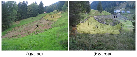
Figure 1. Release area (R) and deposition zone (D) of two of the documented hillslope debris-flow events used for this study [42]. A transition area is not clearly identifiable. Both events occurred in 2005 in Entlebuch (Canton of Lucerne, Switzerland).

An overview of all the events and the selected process parameters is given in Table 1.

Table 1. Characteristics of 19 hillslope debris-flow events in the regions of Appenzell (2002), Entlebuch (2005) and Eriz (2012) in Switzerland, based on event documentations [38,40,41] and soil analysis. The  equivalent friction angle refers to the mean gradient of the flow path, estimated from the distal limits of the source area and deposit of the observed event.

Event ID	Volume	Total Travel Distance	Equivalent Friction Angle	USCS Soil Class	Clay Content
	[m${}^3$]	[m]	[${}^{\circ }$]		[%]
Appenzell, saturated soil conditions assumed
1003	60	43	23	CL	16.0
1005	130	84	22	CL	16.0
1007	800	105	22	CL	16.0
Entlebuch, saturated soil conditions assumed
3001	378	147	19	SC	12.0
3004	280	109	22	SC - SM	8.9
3005	918	208	19	SC	8.1
3007	960	130	22	CL	14.8
3011	392	114	24	SC	14.8
3015	175	53	29	CM	24.0
3017	1050	114	18	SC	12.3
3021	153	53	18	GM	12.0
3028	2800	170	16	-	-
3029	380	121	21	ML $w_L>30$	15.1
Eriz, unsaturated soil conditions assumed
HM1	100	119	18	-	-
HM4	112	72	23	CM	15.5
HM5	91	124	21	SM	8.0
HM6	42	175	26	GC - GM	0.8
HM7	108	136	26	-	-
HM24	655	152	25	GC	9.0

2.2. Evaluation Concept

To quantify the accordance between simulated and observed deposition area, we used the evaluation concept proposed by Heiser et al. [43]. This concept enables an objective comparison and visualisation of model performance across platforms that is independent of process type. The proposed method is based on the comparison of normalised partial observed and simulated areas of deposition (Figure 2), which can be plotted in a ternary diagram to visualise the degree of over- and underestimation. Results are summarised in the single value ${\Omega }_T$:

$${\Omega }_T={\alpha }_T-{\beta }_T-{\gamma }_T$$

(6)

where ${\alpha }_T$ is overlap calculated as $X/T$, ${\beta }_T$ is underestimation calculated as $U/T$ and ${\gamma }_T$ is overestimation as $O/T$ (see Figure 2 for definitions of O, U, X and T). Referring to a receiver operating characteristic (ROC) approach, as, for instance, is applied to analyse the susceptibility of landslide [44] and debris flows [45], X could be defined as the true positives, U as the false negatives and O as the false positives. However, the true negatives are not clearly definable, as the true negatives depend on the simulation perimeter, which is not clearly demarcable—hindering a comparison of the simulation performance of different events. The evaluation concept, based on Equation (6), has the advantage that the possible range of ${\Omega }_T$ is fixed between 1 (indicating a perfect fit) and −1 (total misfit), regardless of the simulation perimeter.

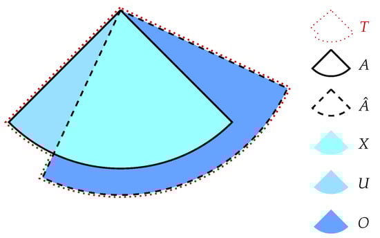
Figure 2. Schematic mass movement deposit distribution with superimposed simulation. A is the observed deposition area (reference situation), whereas $\widehat{A}$ is the total simulated area. O is the size of the overestimated area, whereas U is the size of the underestimated area. X is the area in which the simulation outcome and the reference situation overlap. Finally, T refers to $A\cup \widehat{A}$.

For this study, we applied the evaluation concept to find those friction parameters which are best reproducing the observed deposition area by applying the parameter settings described in Section 2.3. In other words, we performed multiple simulations until the largest ${\Omega }_T$ value for each event and each setting was found.

2.3. Parameter Settings

The aim of this study was to investigate whether the modified Voellmy–Salm model (VS model, Equation (5)) leads to significant improvements in the prediction of the runout behaviour of hillslope debris flows. For this reason, all compiled events were back-calculated based on the standard Voellmy-type shear stress model, defined by $\mu$ and $\xi$ (cf. Equation (4)). No yield stress of the flow was considered for these simulations. To compare the standard VS with the modified VS model, further simulations were performed with the modified shear stress Equation (5)—taking into account the shear stress of the flow $N_0$ as the only calibration parameter. Here, the parameters of the standard Voellmy model were kept constant. The simulations presented in this study are based on the following three parameter settings:

A 

Back-calculation of best-fit friction parameters ${\mu }^{*}$ and ${\xi }^{*}$ without applying a yield stress of the flow $N_0$.

B 

Back-calculation of a best-fit yield stress of the flow $N_0^{*}$ by using mean friction parameters $⟨{\mu }^{*}⟩$ and $⟨{\xi }^{*}⟩$ from simulations based on setting A for each study area (Appenzell, Entlebuch and Eriz).

C 

Back-calculation of a best-fit yield stress of the flow $N_0^{**}$ by using default values of $\mu =0.2$ and $\xi =200$ as proposed by the user manual for RAMMS DF [46].

A classic backward calculation is based on the setting A, where the best-fit Voellmy parameters ${\mu }^{*}$ and ${\xi }^{*}$ were determined.

Setting B applies the mean Voellmy-type shear stress values as given from setting A (${\mu }^{*}$ and ${\xi }^{*}$) to calibrate $N_0^{*}$, the effective yield stress of flow. Finally, default Voellmy-type shear stress values were used in setting C to explore a possible simple method, accounting for the yield stress of the flow $N_0^{**}$ as the only user defined friction parameter in RAMMS DF.

3. Results

A main challenge for simulation models with a physical background is, besides the selection of suitable flow resistance parameters, the definition of an appropriate stopping criteria. In this study, we defined the stopping criteria of the RAMMS DF simulations for each region individually during the first scenario simulations and kept them constant for all subsequent runs. The flow in the model is considered to stop when the percentage of the mass momentum drops below a small constant value which is referenced to the maximum calculated momentum of the flow. The use of such a cut-off momentum criterion increases the objectivity of using the model because the flow often creeps forward at a very low rate (a few cm/s) when it would otherwise be judged to stop when visualising the results.

The stopping criterion for simulations in Entlebuch and Eriz belong to 3.3% and 6.2% of the maximum calculated momentum. Those stopping criteria were defined based on the events Entlebuch-3001 and Eriz-HM1, because they involved undisturbed runout on a uniform slope. Using the default parameters $\mu$ = 0.2 [-] and $\xi$ = 200 [$\mathrm{m}/{\mathrm{s}}^2$], suggested by Bartelt et al. [46], the stopping criteria with the best visual match between the documented and the modelled runout area was chosen. With only three events observed in Appenzell, we applied a constant stopping criteria, which belongs to 5% of the maximum calculated momentum. When running the model, it was assumed that the initial flow starts instantaneously and not as a progressive failure with a series of smaller-volume slumps.

The best-fit values for all parameter settings and hillslope debris-flow events are listed in Table 2.

Table 2. Back-calculated resistance values for all parameter settings used in this study.

Event ID	Setting A		Setting B			Setting C †
	${\mathit{\mu }}^{*}$ [ ]	${\mathit{\xi }}^{*}$[m/s${}^2$]	${\mathit{N}}_0$* [kPa]	$⟨{\mathit{\mu }}^{*}⟩$ [ ]	$⟨{\mathit{\xi }}^{*}⟩$[m/s${}^2$]	${\mathit{N}}_0^{**}$ [kPa]
Appenzell
1003	0.23	200	0.00	0.31	200	0.10
1005	0.40	200	0.20	0.31	200	0.70
1007	0.30	200	0.05	0.31	200	0.25
Entlebuch
3001	0.21	300	0.05	0.30	507	0.05
3004	0.13	240	0.00	0.30	507	0.00
3005	0.11	190	0.00	0.30	507	0.00
3007	0.46	150	1.70	0.30	507	1.60
3011	0.40	285	1.10	0.30	507	1.55
3015	0.49	300	2.75	0.30	507	2.95
3017	0.33	550	0.10	0.30	507	0.60
3021	0.35	1250	1.35	0.30	507	1.50
3028	0.24	700	1.10	0.30	507	0.78
3029	0.33	1100	0.65	0.30	507	0.95
Eriz
HM1	0.20	400	0.00	0.23	446	0.05
HM4	0.37	175	0.30	0.23	446	0.30
HM5	0.05	300	0.00	0.23	446	0.00
HM6	0.05	200	0.00	0.23	446	0.00
HM7	0.40	900	0.19	0.23	446	0.17
HM24	0.29	700	0.65	0.23	446	1.20

† all simulations with $\mu =0.20$ and $\xi =200$, following RAMMS user manual [46].

It is remarkable that the back-calculated velocity-dependent friction parameters $\xi$ of hillslope debris-flow events follow a narrower bandwidth than the dry Coulomb friction criteria in the modelling of hillslope debris-flow events. An example of back-calculated results for all parameter settings of the event HM4 (Eriz)—compared to the observed runout zone—is shown in Figure 3.

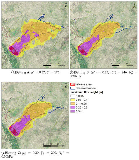
Figure 3. Simulation results of hillslope debris-flow event HM4 (Eriz) for all parameter settings. Observed release area and runout zone are shown with red and blue lines, respectively.

Typical $\mu$ and $\xi$ parameters for different mass movements are plotted in Figure 4 along with the best-fit Voellmy-type friction parameters of the compiled hillslope debris-flow events used in this study (Setting A).

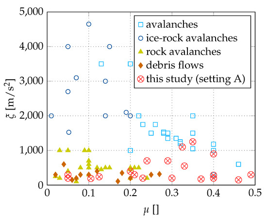
Figure 4. Friction parameters $\mu$ and $\xi$ from back-calculation of different events with RAMMS DF. Avalanche data are from Christen et al. [28], Bartelt et al. [36], Barbolini et al. [47]. Ice-rock avalanche data are from Allen et al. [48], Lipovsky et al. [49] and Schneider et al. [50]. Rock avalanche data are from McKinnon et al. [51], Hungr and Evans [52], Hungr and McDougall [53] and Sosio et al. [54]. Debris flow data are from Scheidl et al. [10], Hürlimann et al. [15], Stricker [55], Evans et al. [56], McDougall [57] and Naef et al. [58]. Hillslope debris-flow events considered in this study are from parameter Setting A described in the text below. All best-fit Voellmy parameters were stated in the respective studies on the basis of a qualitative assessment of performance. However, for a sound review on the applied evaluation concepts of the bibliographical references, we refer to the supplementary material provided by Heiser et al. [43].

3.1. Back-Calculation of Friction Parameters $\mu$ and $\xi$ (Setting A)

For the setting A, all events could be simulated, estimating the best-fit Voellmy-type shear stress parameters $\mu$ and $\xi$ without considering the yield stress of flow.

On average, nearly 50% of depositional zones, predicted by simulations based on the parameter setting A, agree with the observed deposition areas documented in Rickli and Bucher [40], Rickli et al. [41] and Steinemann [38]. However, most simulations also considerably overestimated the lateral spread of the flow, compared to field observations. This is reflected by the large ${\gamma }_T$ value in Table 3. The overall performance in predicting hillslope debris-flow deposition zones based on simulations with setting A, can be given quantitatively with an ${\Omega }_T$ value of -0.05 ± 0.18 (cf. Table 3).

Table 3. Evaluation results for setting A. ${\alpha }_T$ denotes the simulation performance related to the overlap (a value of 1 corresponds to full coverage of simulation/observed). ${\beta }_T$ is a performance measure of the underestimation, whereas ${\gamma }_T$ shows the overestimation performance of the considered simulation. The overall performance is specified by ${\Omega }_T$. All values are calculated based on Equation (6), following the procedure described in Heiser et al. [43].

5cSetting A
	${\mathbf{\alpha }}_{\mathbf{T}}$	${\mathbf{\beta }}_{\mathbf{T}}$	${\mathbf{\gamma }}_{\mathbf{T}}$	${\Omega }_{\mathbf{T}}$
Appenzell
mean value	0.49	0.03	0.48	-0.02
standard deviation	0.06	0.02	0.04	0.12
Entlebuch
mean value	0.48	0.07	0.45	-0.04
standard deviation	0.10	0.08	0.09	0.20
Eriz
mean value	0.45	0.03	0.52	-0.10
standard deviation	0.09	0.04	0.10	0.17
Overall
mean value	0.47	0.05	0.48	-0.05
standard deviation	0.09	0.07	0.09	0.18
sample count	19	19	19	19

3.2. Back-Calculation of Cohesion Parameters $N_0^{*}$ and $N_0^{**}$ (Settings B and C)

Settings B and C have been set up to analyse the simulation performance of RAMMS DF as a function of the yield stress of the flow only. For this reason, we kept the Voellmy-type shear stress parameters $\mu$ and $\xi$ constant.

For parameter setting B we applied the back-calculated mean friction values of parameter setting A for each study site and calibrated event-specific yield stresses of the flow $N_0^{*}$. The calibrated yield stress values of the flow for all events have been found to range between 0.00;2.75 $\mathrm{k}\mathrm{Pa}$ (Table 2), and the mean performance evaluation value for all simulations conducted with setting B amounts to ${\Omega }_T=-0.05$± 0.24 (Table 4).

Table 4. Evaluation results for settings B and C. ${\alpha }_T$ denotes the simulation performance related to the overlap (a value of 1 corresponds to full coverage of simulation/observed). ${\beta }_T$ is a performance measure of the underestimation, whereas ${\gamma }_T$ shows the overestimation performance of the considered simulation. The overall performance is specified by ${\Omega }_T$. All values are calculated based on Equation (6), following the procedure described in Heiser et al. [43].

	Setting B					Setting C
	${\mathbf{\alpha }}_{\mathbf{T}}$	${\mathbf{\beta }}_{\mathbf{T}}$	${\mathbf{\gamma }}_{\mathbf{T}}$	${\Omega }_{\mathbf{T}}$		${\mathbf{\alpha }}_{\mathbf{T}}$	${\mathbf{\beta }}_{\mathbf{T}}$	${\mathbf{\gamma }}_{\mathbf{T}}$	${\Omega }_{\mathbf{T}}$
					Appenzell
mean value	0.48	0.09	0.43	−0.04		0.51	0.03	0.46	0.02
standard deviation	0.03	0.07	0.09	0.07		0.06	0.02	0.04	0.12
					Entlebuch
mean value	0.46	0.16	0.38	−0.08		0.50	0.10	0.40	0.01
standard deviation	0.14	0.15	0.11	0.29		0.11	0.09	0.10	0.22
					Eriz
mean value	0.51	0.12	0.36	0.03		0.52	0.11	0.37	0.04
standard deviation	0.10	0.11	0.15	0.21		0.11	0.11	0.14	0.22
					Overall
mean value	0.48	0.14	0.38	−0.04		0.51	0.09	0.40	0.02
standard deviation	0.12	0.13	0.12	0.24		0.10	0.10	0.11	0.21
sample count	19	19	19	19		19	19	19	19

For parameter setting C, we applied the default friction values—$\mu =0.2$ and $\xi =200$—as proposed by Bartelt et al. [46], which resulted in back-calculated yield stress values of the flow ($N_0^{**}$), ranging from 0.00–2.95 $\mathrm{k}\mathrm{Pa}$ (cf. Table 2).

The average performance of setting C (${\Omega }_T=0.02$±0.24) is higher than those of setting A and setting B. This might be due to lower overestimation ${\gamma }_T$ and better accordance ${\alpha }_T$, despite a similar increased underestimation ${\beta }_T$ (c.f. Figure 5).

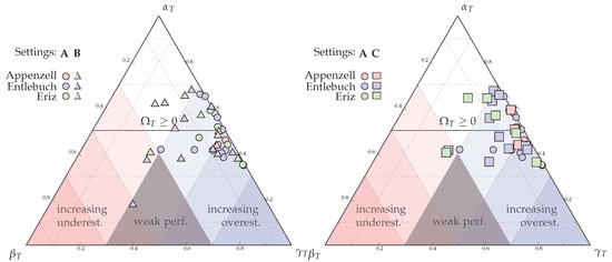
Figure 5. Graphical displays to compare the resulting ${\Omega }_T$ values for the simulation settings A and B (left figure) and A and C (right figure). The right and left increasing colour ranges indicate increasing over- or underestimation of performance (${\gamma }_T,{\beta }_T>30\%$). Weak performance is defined by ${\alpha }_T<40\%$ and ${\gamma }_T,{\beta }_T>30\%$.

4. Discussion and Conclusions

Basically, the overall simulation performance of settings A–C do not differ significantly. Approximately 50% of the observed deposition area is predicted by all simulation settings. We therefore conclude that an additional calibration of $N_0$ does not provide sufficient evidence for a fundamental improvement of the simulation performance. However, in combination with default $\mu$ and $\xi$ values, the yield stress of the flow could be applied as the only user defined flow resistance parameter. Therefore, we see potential, by applying the concept of internal cohesive bonding, especially when it leads to a reduced number of parameters that have to be calibrated.

Simulations based on fixed $\mu$ and $\xi$ values and only calibrating the yield stress of the flow $N_0$—settings B and C—showed 10% and 8% less overestimation of the observed depositional area, respectively. Visually this performance improvement can be seen in Figure 5.

The overall performance values ${\Omega }_T$ for setting B and C is more centralised compared to the related performance values of setting A. Interestingly, the simulation performance does not change significantly even when default friction parameters $\mu$ and $\xi$ (Setting C) are assumed. For inverse modelling reasons, the slight improvement (of overestimation) in predicting the deposition area with parameter settings B and C may motivate future research to consider yield stress of the flow for simulating runout of hillslope debris-flow events, whereas both back-calculated yield stress values of the flow are in a similar range as those empirically found for dense snow avalanches based on snow-chute experiments [31,32,35] (see Table 5).

Table 5. Comparison of averaged yield stress values of the flow $N_0$ and dry Coulomb friction parameters $\mu$ for dense snow avalanches based on snow chute experiments and back-calculated values of setting B and C for this study.

Process	$⟨{\mathit{N}}_0⟩$ [kPa]	$⟨\mathit{\mu }⟩$ [ ]	Study
wet snow experiments †	$0.665\pm 0.688$	$0.41\pm 0.08$	[35]
dry snow experiments †	$0.194\pm 0.140$	$0.30\pm 0.11$	[35]
hillslope debris flows	$0.536\pm 0.735$	$0.28\pm 0.04$	this study, setting B
hillslope debris flows	$0.671\pm 0.773$	$0.20\pm 0.0$	this study, setting C

† based on snow chute experiments conducted by Platzer et al. [31], Platzer et al. [32].

Berger et al. [37] analysed functionality and robustness for rare and extreme debris flows that could not be modelled in the laboratory, by using RAMMS DF applying a constant yield stress of the flow. They reported their best-fit parameter combination, predicting both the debris flow velocities and flow heights, with $\mu =0.00$, $\xi =600$$\mathrm{m}/{\mathrm{s}}^2$ and $N_0=0.5$$\mathrm{k}\mathrm{Pa}$. Because their best-fit simulations showed no influence of the dry Coulomb friction parameter ($\mu =0.00$), they suggested that in the channel the debris is fluidized and the flow is well lubricated.

One might further hypothesise that different saturation conditions, which affect shear strength in the soil, might potentially also affect cohesive interaction of the bulk mixture at low shear rates. Our results, however, indicate that the pre-saturation of the soil does not play a significant role for the simulation of the compiled hillslope debris-flow events with RAMMS DF, because we could not detect any clear differences in the simulation performance between the field sites. Further, the yield stress of the flow $N_0$ does not correlate with the effective cohesion $c^{\prime }$, i.e., the shear stress independent of the normal stress—typically also denoted as yield stress in soil mechanics (Figure 6).

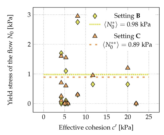
Figure 6. Comparison between back-calculated yield stress values of the flow $N_0^{*}$ and $N_0^{**}$ and effective cohesion $c^{\prime }$ according to the Swiss standard [59] for each soil class.

On the other hand, the back-calculated dry Coulomb friction values ${\mu }^{*}$ show a substantially clear correlation with the percentage clay content in the soil (Figure 7). The same trend can be observed for the yield stress of the flow values $N_0^{*}$ and $N_0^{**}$. These findings support the results of Hürlimann et al. [1]. They observed that the clay content strongly influenced the runout distance and the affected area of experimental hillslope debris flows in the laboratory.

Figure 7. Correlation between back-calculated dry Coulomb friction values $\mu$ and percentage of clay content. The back-calculated yield stress of the flow values based on settings B and C show a similar trend (cf. Table 1 and Table 2).

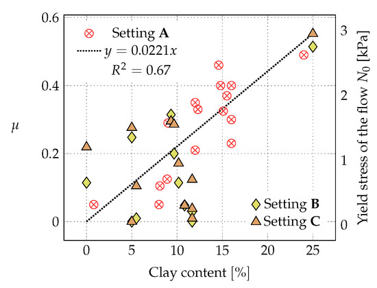
Considering forward modelling, where constitutive parameters have to be known or plausibly assumed, our results show that the yield stress of the flow $N_0$ cannot be determined either by the degree of saturation or by the static yield stress of the soil. A strong correlation, however, can be shown between the dry friction parameter $\mu$ respectively yield stress of the flow $N_0$ and the clay content of the soil.

The numerical simulation program RAMMS intends to offer an easy-to-calibrate tool for the risk delimitation of mass movements. This of course also implies a reduction of the physical basis for the description of complex processes. A reason why the strength of RAMMS cannot be found in a near-natural modelling of the considered process but in a plausible simulation of dynamic prototypical quantities, which form an essential basis for a hazard assessment. Especially for the depositional area of debris-flow-like processes, it has become obvious that beside rheological properties, the topographical conditions have a significant influence on the flow heights, flow velocities and thus on the runout distances.

In any case, note that specifically for hillslope debris flows, runout simulations are based on further assumptions. One uncertainty refers to the estimation of the precise position and size of the release area, which often has a strong influence on simulation results owing to local variations in topography. Furthermore, the consideration of cohesive binding between particles as an additional shear stress represents a strong simplification of the forces acting within a moving mass. Finally, the deposition pattern of a simulation depends on the user-selected stopping criterion. Because the stopping of a hillslope debris flow depends on interactions between fluid and solid components, which are often highly heterogeneous, defining the correct stopping criterion is a problem not yet solved in one component models of the runout of mass movements [60]. It appears that the stopping criterion is also likely to be influenced by the dissolution of the underlying DEM. However, a sensitivity analysis in this respect was outside the scope of this study.

References

- Hürlimann, M.; McArdell, B.W.; Rickli, C. Field and laboratory analysis of the runout characteristics of hillslope debris flows in Switzerland. Geomorphology 2015, 232, 20–32. [Google Scholar] [CrossRef]
- Carrara, A.; Cardinali, M.; Detti, R.; Guzzetti, F.; Pasqui, V.; Reichenbach, P. GIS techniques and statistical models in evaluating landslide hazard. Earth Surf. Process. Landforms 1991, 16, 427–445. [Google Scholar] [CrossRef]
- Fell, R.; Corominas, J.; Bonnard, C.; Cascini, L.; Leroi, E.; Savage, W.Z. Guidelines for landslide susceptibility, hazard and risk zoning for land use planning. Eng. Geol. 2008, 102, 85–98. [Google Scholar] [CrossRef]
- Boll-Bilgot, S.; Gruner, U.; Liniger, M.; Parriaux, A.; Wyss, R. Verbesserung der Hangmurenbeurteilung; Technical Report; Arbeitsgruppe Geologie und Naturgefahren AGN and Abteilung Gefahrenprävention, Bundesamt für Umwelt BAFU: Ittigen, Switzerland, 2016; 149p. [Google Scholar]
- Cislaghi, A.; Bischetti, G.B. Source areas, connectivity, and delivery rate of sediments in mountainous-forested hillslopes: A probabilistic approach. Sci. Total Environ. 2019, 652, 1168–1186. [Google Scholar] [CrossRef] [PubMed]
- Rickenmann, D.; Laigle, D.M.B.W.; McArdell, B.W.; Hübl, J. Comparison of 2D debris-flow simulation models with field events. Comput. Geosci. 2006, 10, 241–264. [Google Scholar] [CrossRef]
- Pastor, M.; Haddad, B.; Sorbino, G.; Cuomo, S.; Drempetic, V. A depth-integrated, coupled SPH model for flow-like landslides and related phenomena. Int. J. Numer. Anal. Methods Geomech. 2009, 33, 143–172. [Google Scholar] [CrossRef]
- Cascini, L.; Cuomo, S.; Pastor, M.; Sorbino, G. Modeling of rainfall-induced shallow landslides of the flow-type. J. Geotech. Geoenviron. Eng. 2010, 136, 85–98. [Google Scholar] [CrossRef]
- Hussin, H.Y.; Quan Luna, B.; Van Westen, C.J.; Christen, M.; Malet, J.P.; van Asch, T.W.J. Parameterization of a numerical 2-D debris flow model with entrainment: A case study of the Faucon catchment, Southern French Alps. Nat. Hazards Earth Syst. Sci. 2012, 12, 3075–3090. [Google Scholar] [CrossRef]
- Scheidl, C.; Rickenmann, D.; McArdell, B. Runout Prediction of Debris Flows and Similar Mass Movements. In Landslide Science and Practice; Margottini, C., Canuti, P., Sassa, K., Eds.; Springer: Berlin/Heidelberg, Germany, 2013; pp. 221–229. [Google Scholar]
- Koo, R.C.H.; Kwan, J.S.H.; Lam, C.; Goodwin, G.R.; Choi, C.E.; Ng, C.W.W.; Yiu, J.; Ho, K.K.S.; Pun, W.K. Back-analysis of geophysical flows using three-dimensional runout model. Can. Geotech. J. 2018, 55, 1081–1094. [Google Scholar] [CrossRef]
- Lateltin, O. Berücksichtigung der Massenbewegungsgefahren bei raumwirksamen Tätigkeiten; Technical Report; Bundesamt für Raumplanung BRP Bundesamt für Wasserwirtschaft BWW Bundesamt für Umwelt, Wald und Landschaft BUWAL: Bern, Switzerland, 1997; 42p. [Google Scholar]
- Hungr, O.; Leroueil, S.; Picarelli, L. The Varnes classification of landslide types, an update. Landslides 2014, 11, 167–194. [Google Scholar] [CrossRef]
- BAFU. Schutz vor Massenbewegungsgefahren. Vollzugshilfe für das Gefahrenmanagement von Rutschungen, Steinschlag und Hangmuren; Technical Report 1608; Bundesamt für Umwelt (BAFU): Ittigen, Switzerland, 2016; 98p. [Google Scholar]
- Hürlimann, M.; Rickenmann, D.; Graph, C. Field and monitoring data of debris-flow events in the Swiss Alps. Can. Geotech. J. 2003, 40, 161–175. [Google Scholar] [CrossRef]
- Iverson, R. The physics of debris flows. Rev. Geophys. 1997, 35, 245–296. [Google Scholar] [CrossRef]
- Iverson, R.M.; Reid, M.E.; LaHusen, R.G. Debris-flow mobilization from landslides. Annu. Rev. Earth Planet. Sci. 1997, 25, 85–138. [Google Scholar] [CrossRef]
- Bollinger, D.; Keusen, H.R.; Rovina, H.; Wildberger, A.; Wyss, R. Gefahreneinstufung Rutschungen i.w.S. Permanente Rutschungen, spontane Rutschungen und Hangmuren; Technical Report; Arbeitsgruppe Geologie und Naturgefahren (AGN) und Bundesamt für Wasser und Geologie: Bern, Switzerland, 2004; 44p. [Google Scholar]
- Christen, M.; Bühler, Y.; Bartelt, P.; Leine, R.I.; Glover, J.; Schweizer, A.; McArdell, B.W.; Gerber, W.; Deubelbeiss, Y.; Feistl, T.; et al. Integral Hazard Management Using a Unified Software Environment Numerical Simulation Tool “RAMMS” for Gravitational Natural Hazards. In Proceedings of the 12th Congress INTERPRAEVENT, Grenoble, France, 23–26 April 2012. [Google Scholar]
- Scheidl, C.; McArdell, B.; Nagl, G.; Rickenmann, D. Debris flow behavior in super- and subcritical conditions. In Proceedings of the Debris-Flow Hazards Mitigation: Mechanics, Monitoring, Modeling, and Assessment, Golden, CO, USA, 10–13 June 2019; Kean, J.W., Coe, J.A., Santi, P.M., Guillen, B.K., Eds.; Association of Environmental and Engineering Geologists: Lexington, KY, USA, 2019. [Google Scholar]
- Cui, P.; Chen, X.; Waqng, Y.; Hu, K.; Li, Y. Jiangia Ravine debris flows in southwestern China. In Debris-flow Hazards and Related Phenomena; Jakob, M., Hungr, O., Eds.; Springer: Berlin/Heidelberg, Germany, 2005; pp. 565–594. [Google Scholar]
- Tecca, P.R.; Galgaro, A.; Genevois, R.; Deganutti, A. Development of a remotely controlled debris flow monitoring system in the Dolomites (Acquabona, Italy). Hydrol. Process. 2003, 17, 1771–1784. [Google Scholar] [CrossRef]
- O’Brien, J.S.; Julien, P.Y.; Fullerton, W.T. Two-dimensional water flood and mudflood simulation. J. Hydraul. Eng. 1993, 119, 244–260. [Google Scholar] [CrossRef]
- Iverson, R.M. Elements of an Improved Model of Debris-flow Motion. AIP Conf. Proc. 2009, 1145, 9–16. [Google Scholar] [CrossRef]
- Mergili, M.; Fischer, J.T.; Krenn, J.; Pudasaini, S.P. r.avaflow v1, an advanced open-source computational framework for the propagation and interaction of two-phase mass flows. Geosci. Model Dev. 2017, 10, 553–569. [Google Scholar] [CrossRef]
- Salm, B.; Burkard, A.; Gubler, H. Berechnung von Fliesslawinen, eine Anleitung für Praktiker mit Beispielen; Mitteilungen des Eidgenössischen Institutes für Schnee und Lawinenforschung, SLF: Davos, Switzerland, 1990; Volume 47. [Google Scholar]
- Salm, B. Flow, flow transition and runout distances of flowing avalanches. Ann. Glaciol. 1993, 18, 221–226. [Google Scholar] [CrossRef]
- Christen, M.; Kowalski, J.; Bartelt, P. RAMMS—Numerical simulation of dense snow avalanches in three-dimensional terrain. Cold Reg. Sci. Technol. 2010, 63, 1–14. [Google Scholar] [CrossRef]
- Christen, M.; Bartelt, P.; Gruber, U. Numerical calculation of snow avalanche runout distances. In Proceedings of the International Conference on Computing in Civil Engineering, Cancun, Mexico, 12–15 July 2005; American Society of Civil Engineers: Reston, VA, USA, 2005; pp. 1–12. [Google Scholar] [CrossRef]
- Voellmy, A. Über die Zerstörungskraft von Lawinen. Schweiz. Bauztg. 1955, 73, 159–162. [Google Scholar]
- Platzer, K.; Bartelt, P.; Kern, M. Measurements of dense snow avalanche basal shear to normal stress ratios (S/N). Geophys. Res. Lett. 2007, 34. [Google Scholar] [CrossRef]
- Platzer, K.; Bartelt, P.; Jaedicke, C. Basal shear and normal stresses of dry and wet snow avalanches after a slope deviation. Cold Reg. Sci. Technol. 2007, 49, 11–25. [Google Scholar] [CrossRef]
- Carson, M.A.; Kirkby, M.J. Hillslope Form and Process; Cambridge University Press: Cambridge, UK, 1972; Volume 475. [Google Scholar]
- Secondi, M.M.; Crosta, G.; Di Prisco, C.; Frigerio, G.; Frattini, P.; Agliardi, F. Landslide motion forecasting by a dynamic viscoplastic model. In Landslide Science and Practice Spatial Analysis and Modelling; Margottini, C., Canuti, P., Sassa, K., Eds.; Springer: Heidelberg, Germany, 2013; pp. 151–159. [Google Scholar]
- Bartelt, P.; Valero, C.V.; Feistl, T.; Christen, M.; Bühler, Y.; Buser, O. Modelling cohesion in snow avalanche flow. J. Glaciol. 2015, 61, 837–850. [Google Scholar] [CrossRef]
- Bartelt, P.; Buehler, Y.; Christen, M.; Deubelbeiss, Y.; Salz, M.; Schneider, M.; Schumacher, L. User Manual v1.7.0—Avalanche. A Numerical Model for Snow Avalanches in Research and Practice; Technical Report; WSL Institute for Snow and Avalanche Research SLF: Birmensdorf, Switzerland, 2017; 126p. [Google Scholar]
- Berger, C.; Christen, M.; Speerli, J.; Lauber, G.; Ulrich, M.; McArdell, B.W. A comparison of physcial and computer-based debris flow modelling of deflection structure at Illgraben, Switzerland. In Proceedings of the 13th Congress INTERPRAEVENT 2016, Lucerne, Switzerland, 30 May–2 June 2016; Koboltschnig, G., Ed.; pp. 212–220. [Google Scholar]
- Steinemann, S. Hillslope Debris-Flow Processes and the Inuence of Geology and its Soil Products. A case study from the Eriz Valley, Switzerland. Ph.D. Thesis, Department of Earth Sciences, ETH Zurich, Zürich, Switzerland, 2013. [Google Scholar]
- Künzi, R.; Hunziker, G.; Krähenbühl, S. Hochwasser vom 4. Juli 2012 in der Zulg; Technical Report; Wald des Kantons Bern, Abteilung Naturgefahren, Interlaken: Bern, Switzerland, 2012; 38p. [Google Scholar]
- Rickli, C.; Bucher, H. Oberflächennahe Rutschungen, ausgelöst durch die Unwetter vom 5.-.16.7. 2002 im Napfgebiet und vom 31.8.-1.9. 2002 im Gebiet Appenzell; Projektbericht, Bundesamtes für Wasser und Geologie BWG: Bern, Switzerland, 2003; 98p. [Google Scholar]
- Rickli, C.; Kamm, S.; Bucher, H. Projektbericht Ereignisanalyse 2005—Teilprojekt Flachgründige Rutschungen; Technical Report; WSL: Birmensdorf, Switzerland, 2008; 114p. [Google Scholar]
- Rickenmann, D. Runout prediction methods. In Debris-Flow Hazards and Related Phenomena; Jakob, M., Hungr, O., Eds.; Springer: Berlin/Heidelberg, Germany, 2005; pp. 305–324. [Google Scholar]
- Heiser, M.; Scheidl, C.; Kaitna, R. Evaluation concepts to compare observed and simulated deposition areas of mass movements. Comput. Geosci. 2017, 21, 335–343. [Google Scholar] [CrossRef][Green Version]
- Frattini, P.; Crosta, G.; Carrara, A. Techniques for evaluating the performance of landslide susceptibility models. Eng. Geol. 2010, 111, 62–72. [Google Scholar] [CrossRef]
- Stancanelli, L.M.; Peres, D.J.; Cancelliere, A.; Foti, E. A combined triggering-propagation modeling approach for the assessment of rainfall induced debris flow susceptibility. J. Hydrol. 2017, 550, 130–143. [Google Scholar] [CrossRef]
- Bartelt, P.; Buehler, Y.; Christen, M.; Deubelbeiss, Y.; Graf, C.; McArdell, B.W.; Salz, M.; Schneider, M. User Manual v1.5—Debris Flow. A Numerical Model for Debris Flows in Research and Practice; Technical Report; WSL Institute for Snow and Avalanche Research SLF: Birmensdorf, Switzerland, 2013; 126p. [Google Scholar]
- Barbolini, M.; Gruber, U.; Keylock, C.J.; Naaim, M.; Savi, F. Application of statistical and hydraulic-continuum dense-snow avalanche models to five real European sites. Cold Reg. Sci. Technol. 2000, 31, 133–149. [Google Scholar] [CrossRef]
- Allen, S.K.; Schneider, D.; Owens, I.F. First approaches towards modelling glacial hazards in the Mount Cook region of New Zealand’s Southern Alps. Nat. Hazards Earth Syst. Sci. 2009, 9, 481–499. [Google Scholar] [CrossRef]
- Lipovsky, P.S.; Evans, S.G.; Clague, J.J.; Hopkinson, C.; Couture, R.; Bobrowsky, P.; Ekström, G.; Demuth, M.N.; Delaney, K.B.; Roberts, N.J.; et al. The July 2007 rock and ice avalanches at Mount Steele, St. Elias Mountains, Yukon, Canada. Landslides 2008, 5, 445–455. [Google Scholar] [CrossRef]
- Schneider, D.; Bartelt, P.; Caplan-Auerbach, J.; Christen, M.; Huggel, C.; McArdell, B.W. Insights into rock-ice avalanche dynamics by combined analysis of seismic recordings and a numerical avalanche model. J. Geophys. Res. Earth Surf. 2010, 115. [Google Scholar] [CrossRef]
- McKinnon, M.; Hungr, O.; McDougall, S. Dynamic analyses of Canadian landslides. In Proceedings of the Fourth Canadian Conference on GeoHazards: From Causes to Management, Québec, QC, Canada, 20–24 May 2008; Locat, J., Perret, D., Turmel, D., Leroueil, S., Demers, D., Eds.; Presse de l’Université Laval: Québec, QC, Canada, 2008; pp. 20–24. [Google Scholar]
- Hungr, O.; Evans, S.G. Rock avalanche runout prediction using a dynamic model. In Proceedings of the 7th International Symposium on Landslides, Trondheim, Norway, 17–21 June 1996; Senneset, K., Ed.; Balkema: Rotterdam, The Netherlands, 1996; Volume 1, pp. 233–238. [Google Scholar]
- Hungr, O.; McDougall, S. Two numerical models for landslide dynamic analysis. Comput. Geosci. 2009, 35, 978–992. [Google Scholar] [CrossRef]
- Sosio, R.; Crosta, G.B.; Hungr, O. Complete dynamic modeling calibration for the Thurwieser rock avalanche (Italian Central Alps). Eng. Geol. 2008, 100, 11–26. [Google Scholar] [CrossRef]
- Stricker, T. Murgänge im Torrente Riascio (TI): Ereignisanalyse, Auslösefaktoren und Simulation von Ereignissen mit RAMMS. Master’s Thesis, University of Zürich, Zürich, Switzerland, 2010. [Google Scholar]
- Evans, S.G.; Guthrie, R.H.; Roberts, N.J.; Bishop, N.F. The disastrous 17 February 2006 rockslide-debris avalanche on Leyte Island, Philippines: A catastrophic landslide in tropical mountain terrain. Nat. Hazards Earth Syst. Sci. 2007, 7, 89–101. [Google Scholar] [CrossRef]
- McDougall, S. A New Continuum Dynamic Model for the Analysis of Extremely Rapid Landslide Motion across Complex 3d Terrain. Ph.D. Thesis, The University of British Columbia, Vancouver, BC, USA, 2006. [Google Scholar]
- Naef, D.; Rickenmann, D.; Rutschmann, P.; McArdell, B.W. Comparison of flow resistance relations for debris flows using a one-dimensional finite element simulation model. Nat. Hazards Earth Syst. Sci. 2006, 6, 155–165. [Google Scholar] [CrossRef]
- Bodenkennziffern. Schweizerischer Verband der Strassen-und Verkehrsfachleute (VSS); SN 670 010b; Swiss Association for Standardization (SNV): Zürich, Switzerland, 1998. [Google Scholar]
- Bühler, Y. RAMMS—RApid Mass MovementS. Background Information. 2011. Available online: https://ramms.slf.ch/ramms/index.php?option=com_content&view=article&id=57&Itemid=74 (accessed on 7 November 2011).
© 2020 by the authors. Licensee MDPI, Basel, Switzerland. This article is an open access article distributed under the terms and conditions of the Creative Commons Attribution (CC BY) license (http://creativecommons.org/licenses/by/4.0/).