Simple Particle Model for Low-Density Granular Flow Interacting with Ambient Fluid


Abstract
:1. Introduction
2. Methods
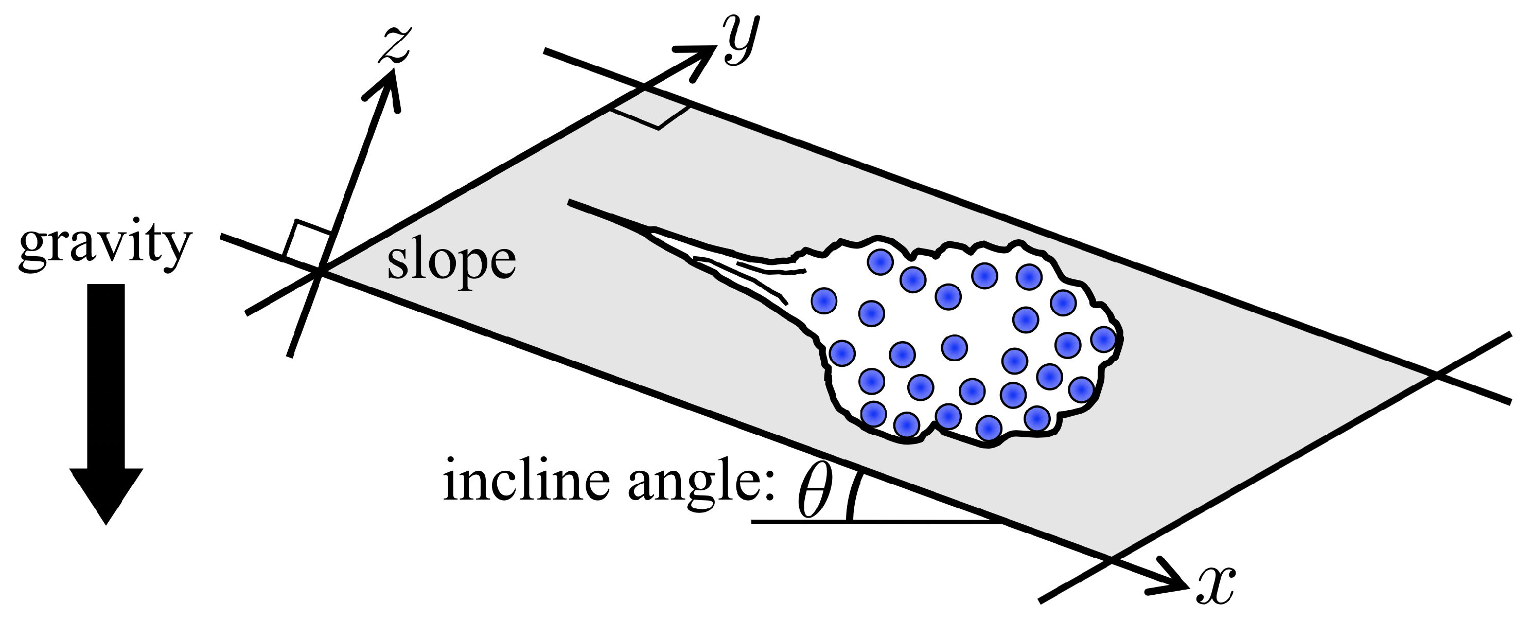
2.1. Concept of the Proposed Model
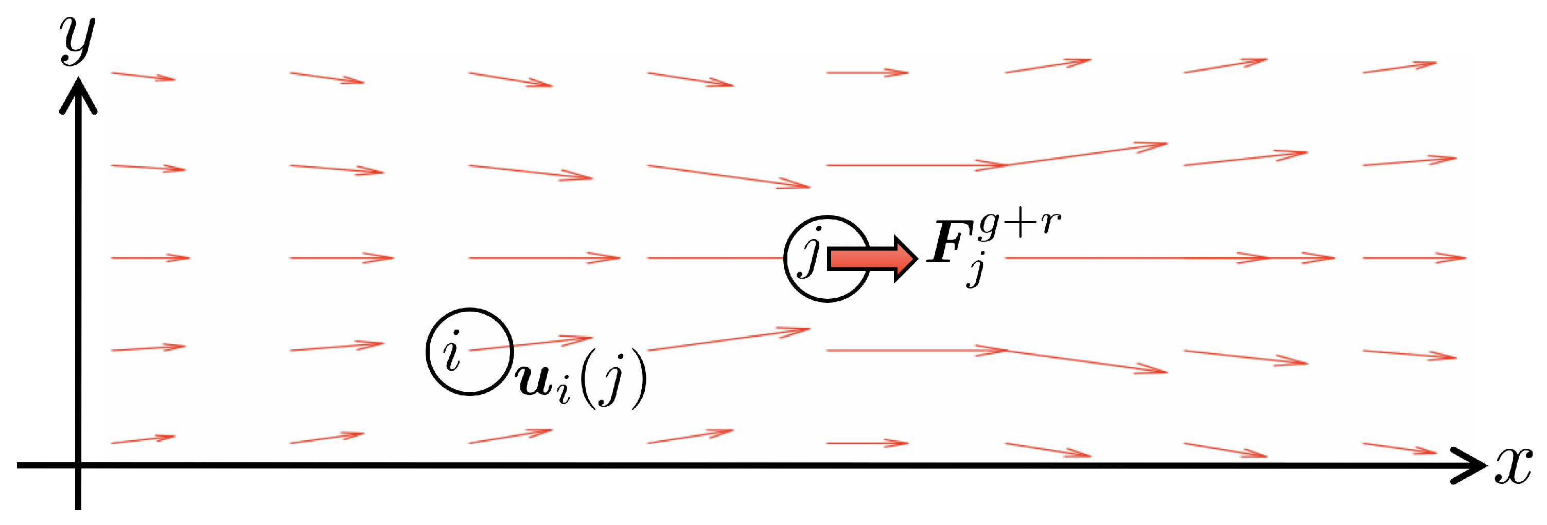
2.2. Particle Model
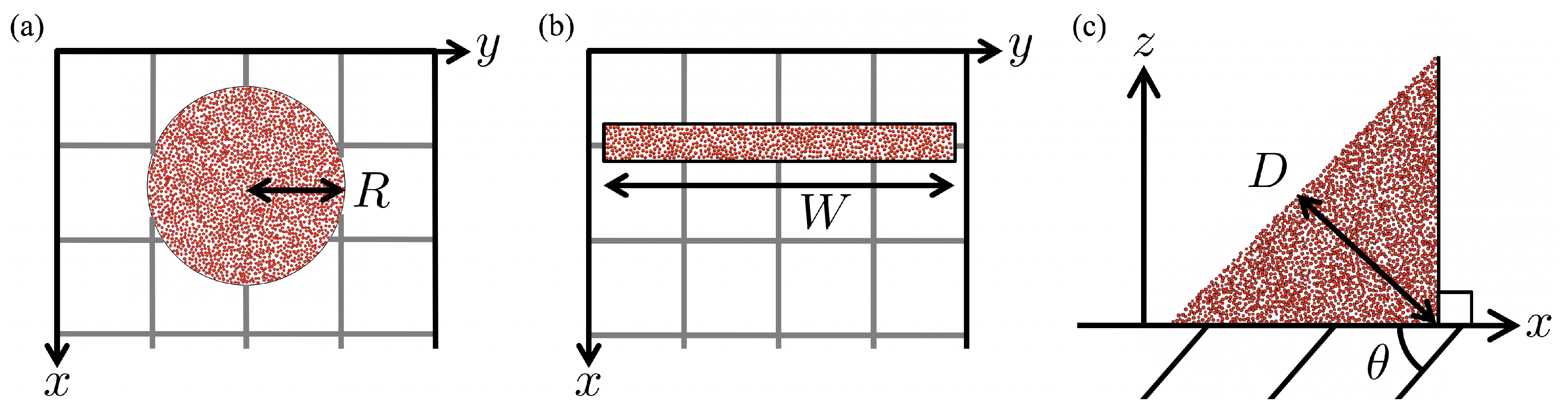
2.3. Simulation Setup
2.4. Nondimensionalization of the Proposed Model
3. Results
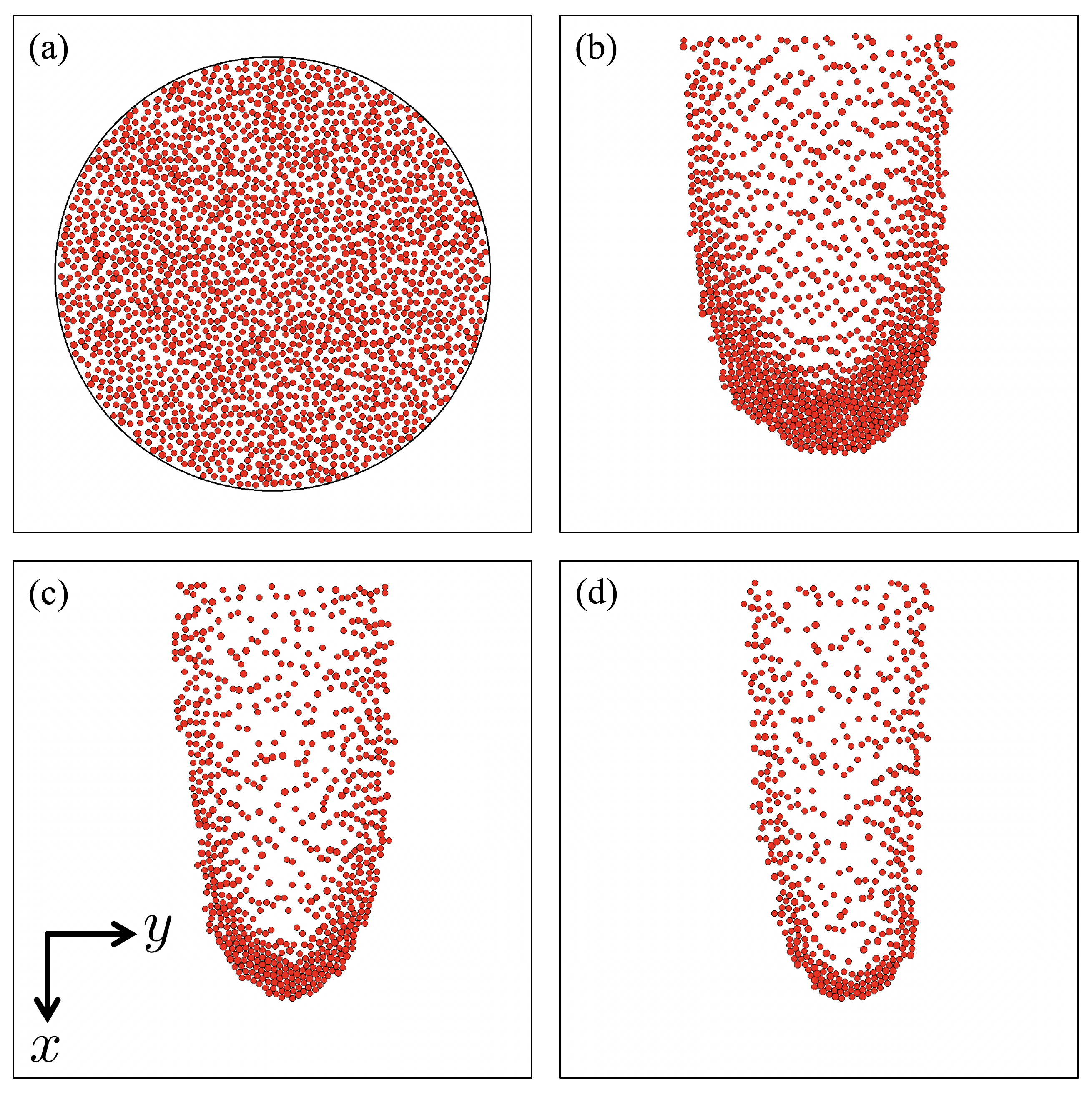
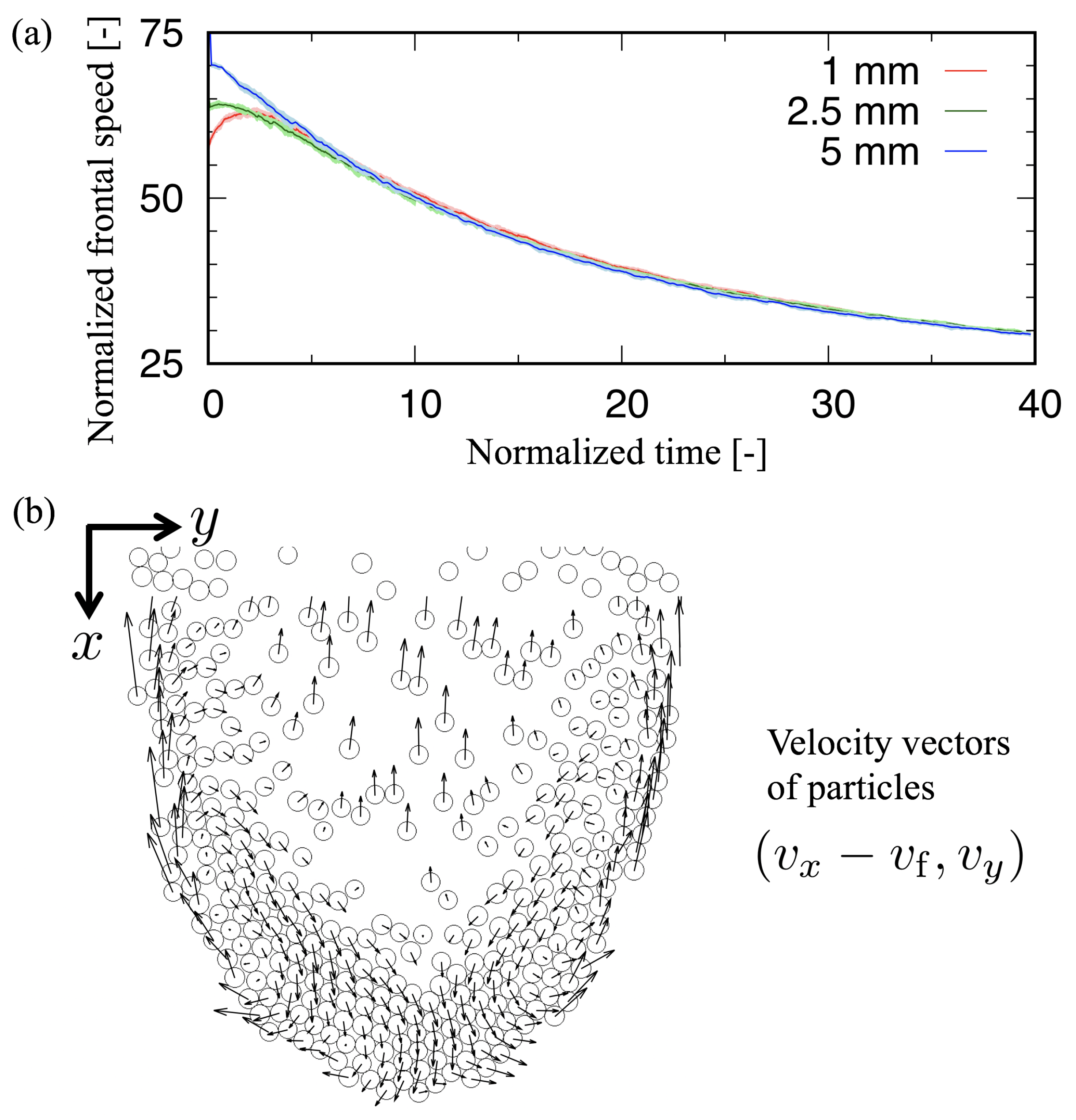
3.1. Circular Shape in the x–y Plane
3.2. Rectangular Shape in the x–y Plane
3.3. Triangular Shape in the x–z Plane
4. Discussion
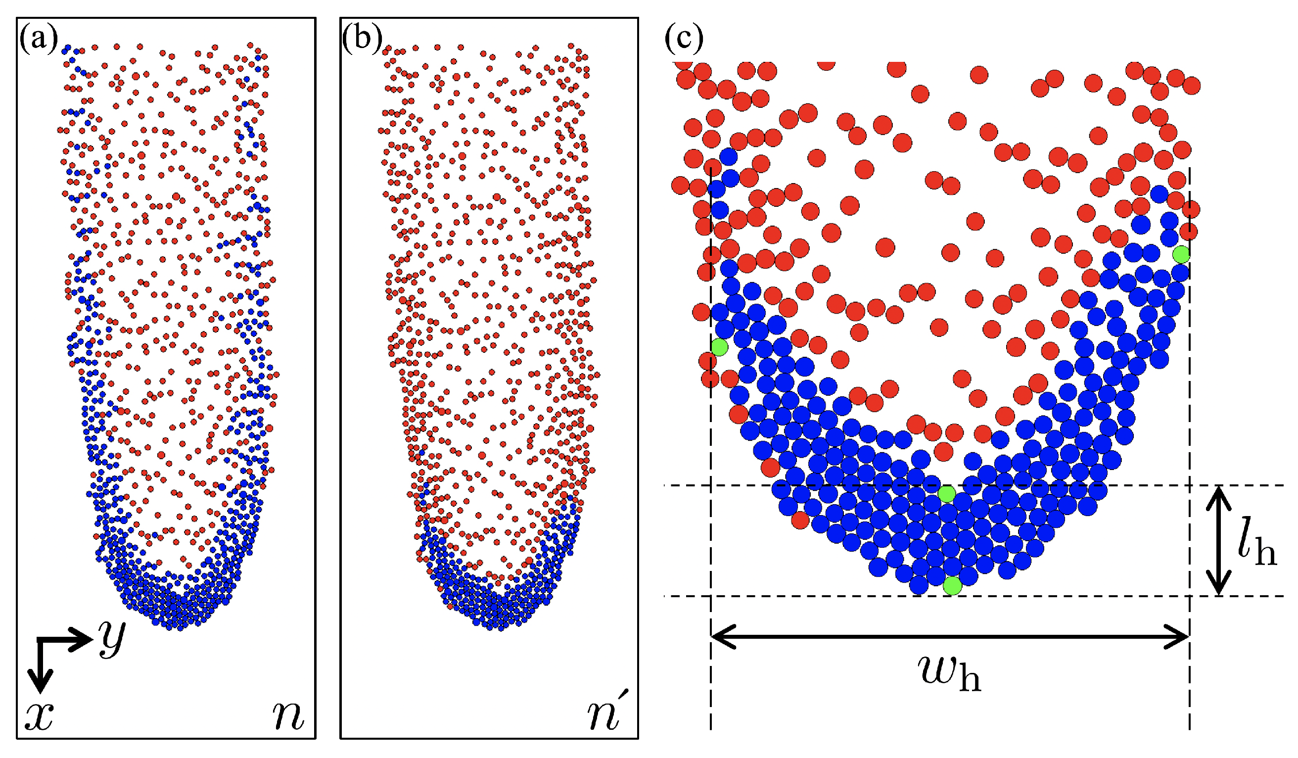
4.1. Definition of the Head in the x–y Plane
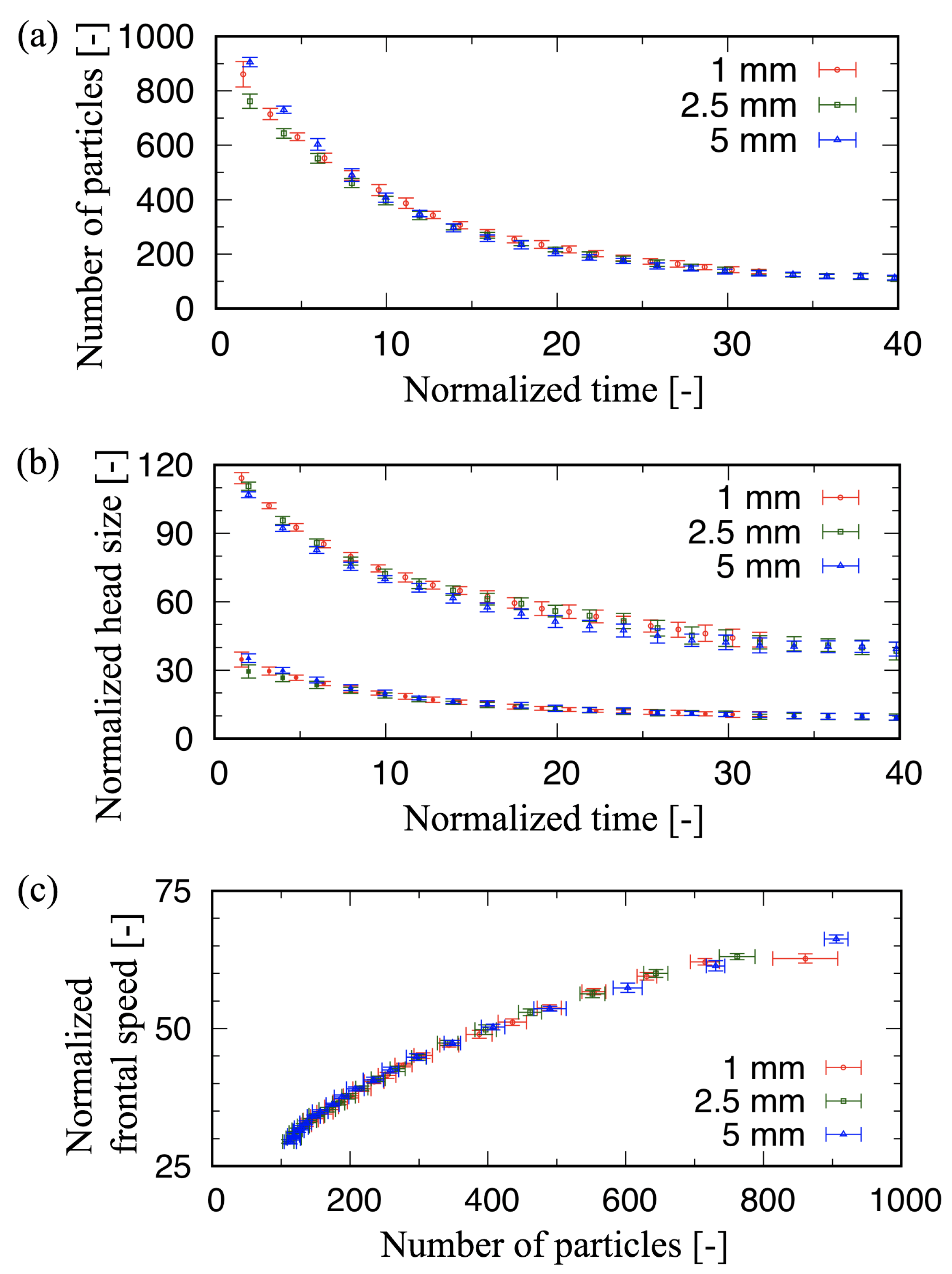
4.2. Characteristics of Head Size in the x–y Plane
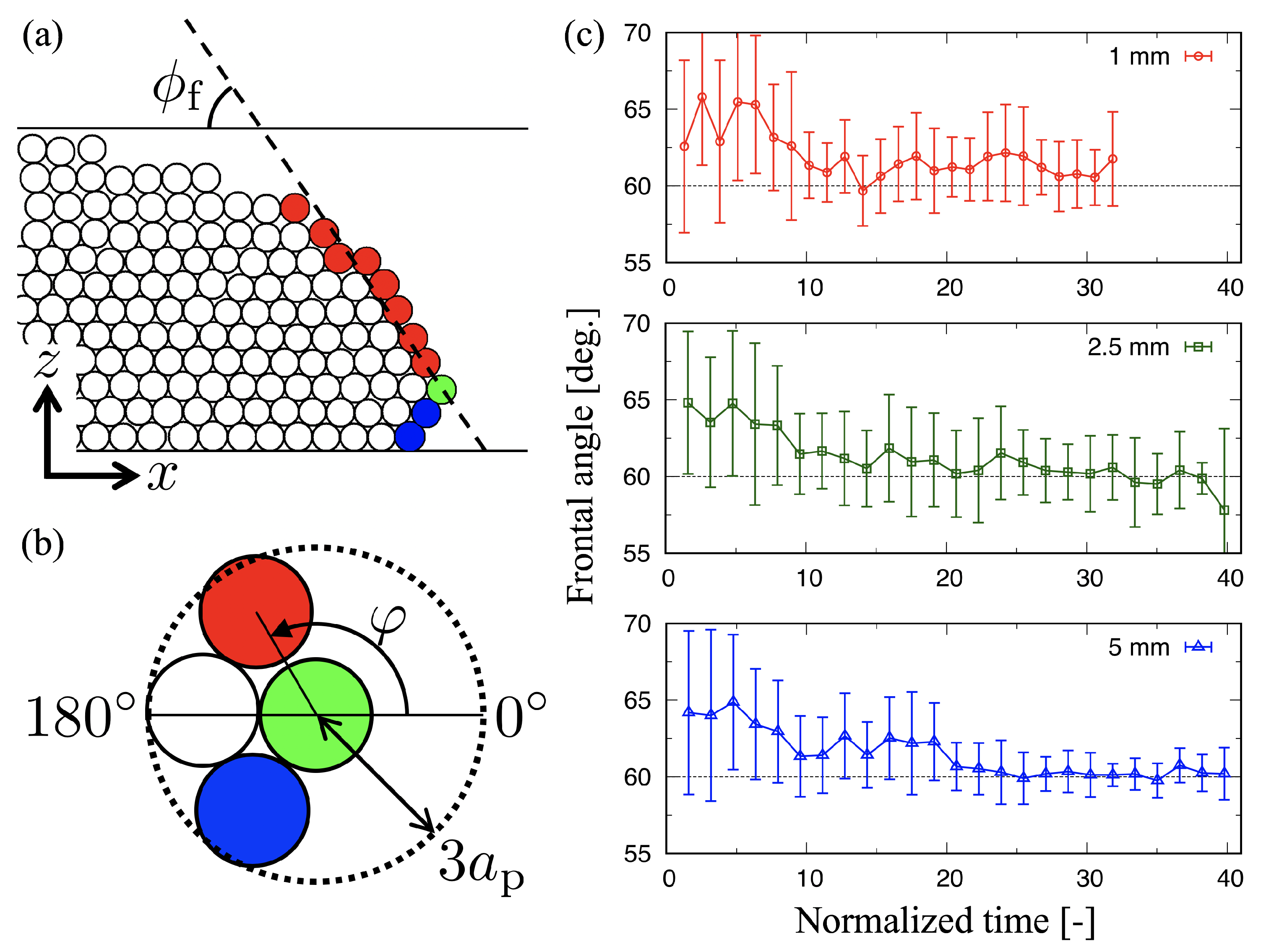
4.3. Frontal Angle in the x–z Plane
5. Conclusions
Author Contributions
Funding
Acknowledgments
Conflicts of Interest
References
- Sovilla, B.; McElwaine, J.N.; Louge, M.Y. The structure of powder snow avalanches. C. R. Physique 2015, 16, 97–104. [Google Scholar] [CrossRef]
- Köhler, A.; McElwaine, J.; Sovilla, B.; Ash, M.; Brennan, P. The dynamics of surges in the 3 February 2015 avalanches in Vallée de la Sionne. J. Geophys. Res. Earth Surf. 2016, 121, 2192–2210. [Google Scholar] [CrossRef] [Green Version]
- Iverson, R.M. The physics of debris flows. Rev. Geophys. 1997, 35, 245–296. [Google Scholar] [CrossRef] [Green Version]
- Pouliquen, O.; Delour, J.; Savage, S.B. Fingering in granular flows. Nature 1997, 386, 816–817. [Google Scholar] [CrossRef]
- Forterre, Y.; Pouliquen, O. Longitudinal vortices in granular flows. Phys. Rev. Lett. 2001, 86, 5886–5889. [Google Scholar] [CrossRef] [PubMed] [Green Version]
- Tiefenbacher, F.; Kern, M.A. Experimental devices to determine snow avalanche basal friction and velocity profiles. Cold Reg. Sci. Technol. 2004, 38, 17–30. [Google Scholar] [CrossRef]
- Gray, J.M.N.T.; Ancey, C. Segregation, recirculation and deposition of coarse particles near two-dimensional avalanche fronts. J. Fluid Mech. 2009, 629, 387–423. [Google Scholar] [CrossRef]
- Gray, J.; Ancey, C. Multi-component particle-size segregation in shallow granular avalanches. J. Fluid Mech. 2011, 678, 535–588. [Google Scholar] [CrossRef] [Green Version]
- Fischer, J.T.; Kaitna, R.; Heil, K.; Reiweger, I. The Heat of the Flow: Thermal Equilibrium in Gravitational Mass Flows. Geophys. Res. Lett. 2018, 45, 219–226. [Google Scholar] [CrossRef] [Green Version]
- Thompson, P.A.; Grest, G.S. Granular flow: Friction and the dilatancy transition. Phys. Rev. Lett. 1991, 67, 1751–1754. [Google Scholar] [CrossRef]
- Silbert, L.E.; Ertas, D.; Grest, G.S.; Halsey, T.C.; Levine, D.; Plimpton, S.J. Granular flow down an inclined plane: Bagnold scaling and rheology. Phys. Rev. E 2001, 64, 051302. [Google Scholar] [CrossRef] [PubMed] [Green Version]
- Savage, S.B.; Hutter, K. The motion of a finite mass of granular material down a rough incline. J. Fluid Mech. 1989, 199, 177–215. [Google Scholar] [CrossRef]
- Forterre, Y.; Pouliquen, O. Stability analysis of rapid granular chute flows: formation of longitudinal vortices. J. Fluid Mech. 2002, 467, 361–387. [Google Scholar] [CrossRef] [Green Version]
- Pitman, E.B.; Nichita, C.C.; Patra, A.; Bauer, A.; Sheridan, M.; Bursik, M. Computing granular avalanches and landslides. Phys. Fluids 2003, 15, 3638. [Google Scholar] [CrossRef] [Green Version]
- Patra, A.K.; Bauer, A.C.; Nichita, C.C.; Pitman, E.B.; Sheridan, M.F.; Bursik, M.; Rupp, B.; Webber, A.; Stinton, A.J.; Namikawa, L.M.; et al. Parallel adaptive numerical simulation of dry avalanches over natural terrain. J. Volcanol. Geotherm. Res. 2005, 139, 1–21. [Google Scholar] [CrossRef]
- Pailha, M.; Pouliquen, O. A two-phase flow description of the initiation of underwater granular avalanches. J. Fluid Mech. 2009, 633, 115–135. [Google Scholar] [CrossRef]
- Beghin, P.; Hopfinger, E.J.; Britter, R.E. Gravitational convection from instantaneous sources on inclined boundaries. J. Fluid Mech. 1981, 107, 407–422. [Google Scholar] [CrossRef]
- Beghin, P.; Olagne, X. Experimental and theoretical study of the dynamics of powder snow avalanches. Cold Reg. Sci. Technol. 1991, 19, 317–326. [Google Scholar] [CrossRef]
- Nishimura, K.; Keller, S.; McElwaine, J.; Nohguchi, Y. Ping-pong ball avalanche at a ski jump. Granul. Matter 1998, 1, 51–56. [Google Scholar] [CrossRef]
- McElwaine, J.; Nishimura, K. Ping-pong ball avalanche experiments. Ann. Glaciol. 2001, 32, 135–148. [Google Scholar] [CrossRef] [Green Version]
- Tischer, M.; Bursik, M.I.; Pitman, E.B. Kinematics of Sand Avalanches Using Particle-Image Velocimetry. J. Sediment. Res. 2001, 71, 355–364. [Google Scholar] [CrossRef]
- Turnbull, B.; McElwaine, J.N. Experiments on the non-Boussinesq flow of self-igniting suspension currents on a steep open slope. J. Geophys. Res. Earth Surf. 2008, 113. [Google Scholar] [CrossRef] [Green Version]
- Nohguchi, Y.; Ozawa, H. On the vortex formation at the moving front of lightweight granular particles. Physica D 2009, 238, 20–26. [Google Scholar] [CrossRef]
- Jackson, A.; Turnbull, B.; Munro, R. Scaling for lobe and cleft patterns in particle-laden gravity currents. Nonlin. Processes Geophys. 2013, 20, 121–130. [Google Scholar] [CrossRef] [Green Version]
- Jackson, A.; Turnbull, B. Identification of particle-laden flow features from wavelet decomposition. Physica D 2017, 361, 12–27. [Google Scholar] [CrossRef] [Green Version]
- Metzger, B.; Nicolas, M.; Guazzelli, E. Falling clouds of particles in viscous fluids. J. Fluid Mech. 2007, 580, 283–301. [Google Scholar] [CrossRef]
- Issler, D. Modelling of snow entrainment and deposition in powder-snow avalanches. Ann. Glaciol. 1998, 26, 253–258. [Google Scholar] [CrossRef] [Green Version]
- Naaim, M.; Gurer, I. Two-phase numerical model of powder avalanche theory and application. Nat. Hazards 1998, 17, 129–145. [Google Scholar] [CrossRef]
- Hartel, C.; Meiburg, E.; Necker, F. Analysis and direct numerical simulation of the flow at a gravity-current head. Part 1. Flow topology and front speed for slip and no-slip boundaries. J. Fluid Mech. 2000, 418, 189–212. [Google Scholar] [CrossRef] [Green Version]
- Hartel, C.; Carlsson, F.; Thunblom, M. Analysis and direct numerical simulation of the flow at a gravity-current head. Part 2. The lobe-and-cleft instability. J. Fluid Mech. 2000, 418, 213–229. [Google Scholar] [CrossRef]
- Ancey, C. Powder snow avalanches: Approximation as non-Boussinesq clouds with a Richardson number–dependent entrainment function. J. Geophys. Res. 2004, 109. [Google Scholar] [CrossRef] [Green Version]
- McElwaine, J.N. Rotational flow in gravity current heads. Phil. Trans. R. Soc. A 2005, 363, 1603–1623. [Google Scholar] [CrossRef] [PubMed]
- Turnbull, B.; McElwaine, J.N. Potential flow models of suspension current air pressure. Ann. Glaciol. 2010, 51, 113–122. [Google Scholar] [CrossRef] [Green Version]
- Espath, L.F.R.; Pinto, L.C.; Laizet, S.; Silvestrini, J.H. High-fidelity simulations of the lobe-and-cleft structures and the deposition map in particle-driven gravity currents. Phys. Fluids 2015, 27, 056604. [Google Scholar] [CrossRef] [Green Version]
- Rotne, J.; Prager, S. Variational treatment of hydrodynamic interaction in polymers. J. Chem. Phys. 1969, 50, 4831. [Google Scholar] [CrossRef]


© 2020 by the authors. Licensee MDPI, Basel, Switzerland. This article is an open access article distributed under the terms and conditions of the Creative Commons Attribution (CC BY) license (http://creativecommons.org/licenses/by/4.0/).
Share and Cite
Niiya, H.; Awazu, A.; Nishimori, H. Simple Particle Model for Low-Density Granular Flow Interacting with Ambient Fluid. Geosciences 2020, 10, 69. https://doi.org/10.3390/geosciences10020069
Niiya H, Awazu A, Nishimori H. Simple Particle Model for Low-Density Granular Flow Interacting with Ambient Fluid. Geosciences. 2020; 10(2):69. https://doi.org/10.3390/geosciences10020069
Chicago/Turabian StyleNiiya, Hirofumi, Akinori Awazu, and Hiraku Nishimori. 2020. "Simple Particle Model for Low-Density Granular Flow Interacting with Ambient Fluid" Geosciences 10, no. 2: 69. https://doi.org/10.3390/geosciences10020069
APA StyleNiiya, H., Awazu, A., & Nishimori, H. (2020). Simple Particle Model for Low-Density Granular Flow Interacting with Ambient Fluid. Geosciences, 10(2), 69. https://doi.org/10.3390/geosciences10020069