Article

Cascading Dynamics of the Hydrologic Cycle in California Explored through Observations and Model Simulations

Jet Propulsion Laboratory, California Institute of Technology, CA 91125, USA
*
Author to whom correspondence should be addressed.
Geosciences 2020, 10(2), 71; https://doi.org/10.3390/geosciences10020071
Submission received: 3 January 2020 / Revised: 3 February 2020 / Accepted: 9 February 2020 / Published: 14 February 2020
(This article belongs to the Special Issue Groundwater in arid and semiarid areas)

Abstract

:
As drought occurs in a region it can have cascading effects through the water cycle. In this study, we explore the temporal co-evolution of various components of the hydrologic cycle in California from 2002 to 2018. We combine information from the Gravity Recovery and Climate Experiment (GRACE) satellites, the North American Land Data Assimilation System (NLDAS) suite of models, and the California Department of Water Resources (DWR) reservoir levels to analyze dynamics of Total Water Storage (TWS), soil moisture, snow pack, large reservoir storage, and ultimately, groundwater. For TWS, a trend of −2 cm/yr is observed during the entire time period of our analysis; however, this rate increases to about −5 cm/yr during drought periods (2006−2010 and 2012−2016). Results indicate that the majority of the loss in TWS is caused by groundwater depletion. Using proper error accounting, we are able to identify the start, the peak, and the ending of the drought periods for each individual water state variable in the study domain. We show that snow and soil moisture are impacted earlier and recover faster than surface water and groundwater. The annual and year-to-year dynamics shown in our results portray a clear cascading effect of the hydrologic cycle on the scale of 8−16 months.

1. Introduction

In recent decades, the demands of fresh water for urban, agricultural, and environmental uses have exceeded the natural renewable supply in many regions of the world, especially for arid and semi-arid regions such as California [1,2]. To date, this gap between the available surface water supply and the growing water demand has caused significant stresses on fresh water systems globally. This has created a large reliance on groundwater, a slowly renewable resource conveniently stored at shallow subsurface aquifer layers. Because of continued extraction and insufficient recharge that is complicated by climate variability (i.e., droughts), depletion of subsurface aquifers has become a dire environmental consequence that is being observed globally in arid and semi-arid regions with highly variable precipitation (e.g., [3,4,5,6,7,8,9,10,11,12]). Generally, various aspects of the hydrologic cycle, such as snow pack and soil moisture, have been impacted by increasing temperatures and more variable precipitation. This overall shock to the water cycle can be seen in both observations and model simulations of total water storage for many regions of the world [7,8,9,10,11,12].
Despite the critical need for fresh water supplies, water resource availability is often poorly monitored. For example, groundwater monitoring networks do not exist at the same scope and scale for those that track surface water [13]. Conventionally, groundwater level change is monitored through in situ measurements at observational wells, which are sparse, very cost ineffective, and difficult to access. Furthermore, measurement records are often discontinuous. To overcome these challenges, various methods, such as geostatistical interpolation and hydrologic model simulation, have been proposed to estimate fresh water availability [14,15]. Even though hydrologic models may be capable of inferring water availability at high spatiotemporal resolution, the conventional land surface models, such as Noah-MP [16], omit consideration of human activities. This lack of representation could cause biases in simulations, for example by underestimating rates of groundwater loss [17]. In addition to groundwater, other sources of fresh water are hardly monitored or tracked, such as soil moisture or snow water. Although methods exist to gather data on these processes, such as airborne or satellite observations, in situ observations, or methods like data assimilation that fuse observations with model simulations [15,18,19], detailed knowledge about the state of these systems is still lacking. This causes a great deal of uncertainty in estimates of the different aspects of the hydrologic cycle.
In California, particularly in productive agricultural regions such as the Central Valley, has experienced periodic declines in total water storage in recent decades. A main reason for the loss of fresh water in this region is due to groundwater depletion. Annually, at least 40% or more of the Central Valley’s demand for water is supplied from groundwater, with the majority is used in agriculture [11,20] Data from the United States Geological Survey (USGS) show that between 1962 and 2003, groundwater use in the Central Valley increased from 0.75 to 2.5 km3 per year [21]. The groundwater extracted for irrigation often exceeds the natural recharge, leading to declines in the groundwater table [13,21,22,23]. Furthermore, the winter snow pack in the Sierra Nevada is usually a reliable source of fresh water for the drier spring and summer seasons. However, recent years have shown a large increase in temperatures and a slight decrease in precipitation, causing a depletion of the snowpack for many regions where snow is usually available [15]. Also, large surface water reservoirs have shown periods of depleted reserves during droughts, and many of the largest reservoirs were in critical condition during recent droughts [24]. The impacts from droughts are usually felt in one hydrologic process before it reaches another, for example, depletion of the snow pack occurs before groundwater reserves are relied on. In this study, we aim to capture this cascading effect of the hydrologic cycle for California, and to quantify its uncertainty by analyzing different sources of information that are available.
More recently, much effort has been focused on monitoring aspects of the hydrologic cycle using remote sensing techniques (e.g., [4,5,7,13,25,26,27]). For example, NASA’s Gravity Recovery and Climate Experiment (GRACE) mission [28] has proven to be an extremely valuable tool for regional to global scale water cycle studies [7,28]. Satellite observations of Earth’s gravity field from GRACE are processed routinely into estimates of surface mass change and can provide information about basin-scale dynamics of groundwater. GRACE mass change estimates can be combined with other hydrologic information, such as model simulations or in situ observations, to infer groundwater changes (e.g., [7,11,12,13,29,30]). For example, information on snow and soil moisture can be obtained from high-resolution land surface models, and reservoir storage information can be obtained by local water managers, and this information can be helpful to estimate groundwater dynamics derived from the GRACE satellites. In this way, various sources of information are fused to quantify the water cycle along with its uncertainty.
Total Water Storage (TWS) estimates from GRACE include all of the snow, ice, surface water, soil water, canopy water, and groundwater in a region, and when combined with auxiliary hydrologic datasets, TWS can be utilized to infer process information on groundwater, or other water sources. To investigate the various water processes in our study, we utilize data from the North American Land Data Assimilation System (NLDAS-2) for outputs of soil moisture and snow water equivalent [19,31]. For surface water, we use data from the California Department of Water Resources (DWR) on the 50 largest reservoirs in the state. We ignore smaller terms that may be negligible, such as ice or canopy water. This leaves us with the groundwater component. By combining all of these sources of information, we can investigate the temporal evolution of each water process and answer questions such as: 1) Is there a cascading effect in the hydrologic cycle that can be clearly extracted from the data? 2) Are there obvious differences in the timing of drought (beginning, peak and end of drought) for each process, and if so, by how many months (or years)? By utilizing the various sources of information available to us via satellite observations, model simulations, and ground observations, we are able to infer the cascading effect of the water cycle and can make quantitative assessments of the evolution of each hydrologic process.

2. Data and Methods

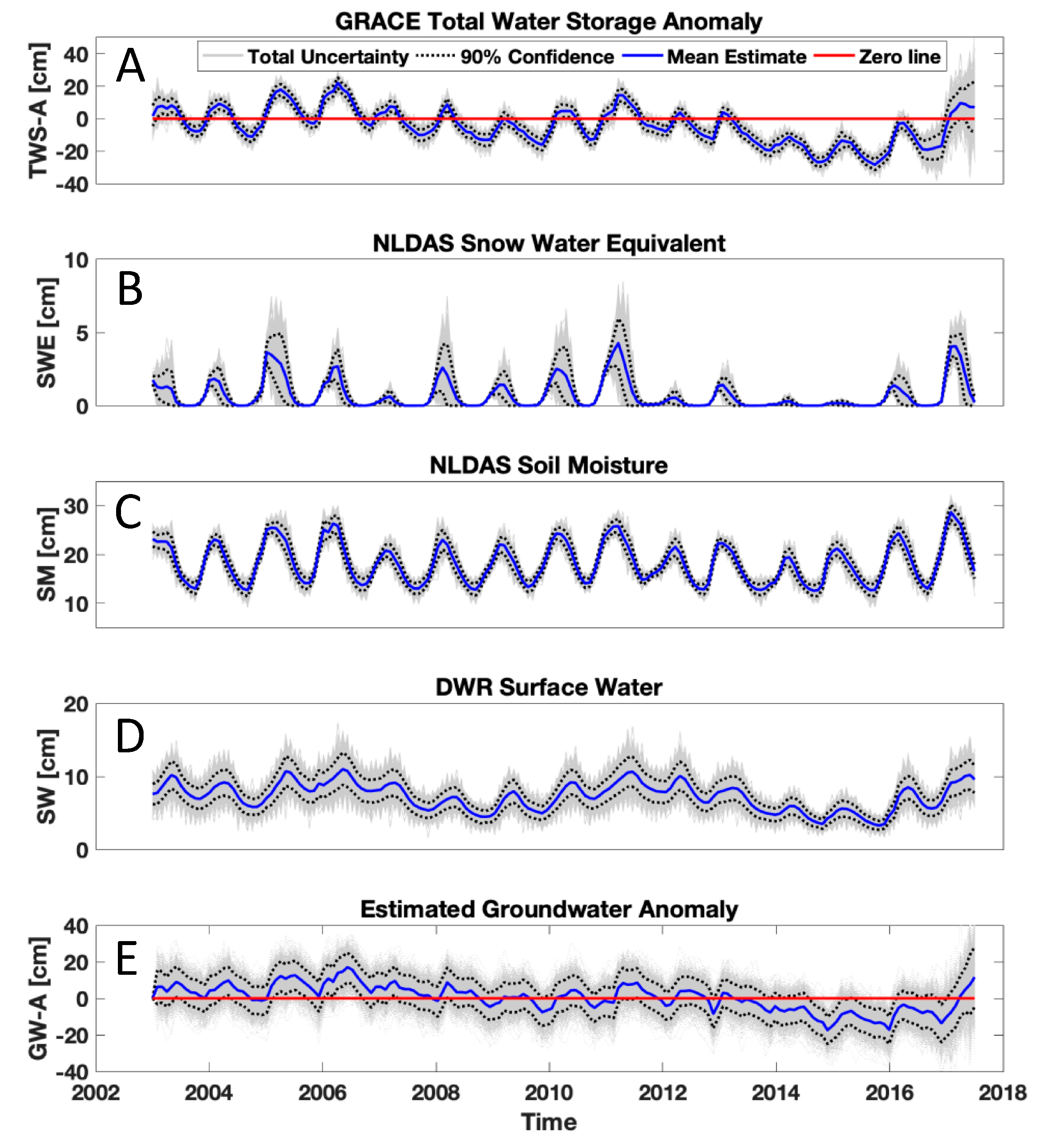
2.1. GRACE Satellites

NASA’s Gravity Recovery and Climate Experiment (GRACE) satellite mission provided a new means to observe fresh water variability from space (e.g., [5,7,13,29]). Since 2003, satellite observations of time variable gravity from the GRACE mission have provided monthly estimates of total mass change globally. These estimates have been widely used for hydrology and water resource monitoring.
Various recent studies have demonstrated that GRACE derived estimates of variations of total water storage (TWS) can provide fresh water availability estimates with sufficient accuracy [11,18,26]. These GRACE-based methods have been applied to regions such as Northern India [5,32], the Middle East [33,34], Northern China [35,36], and California [7,11,13,30], among others. In this study, the JPL RL05M.1 Version 2 GRACE mascon product, which can be downloaded at https://grace.jpl.nasa.gov/data/get-data/ [37,38], is used to examine water storage changes in California (Figure 1) and its underlying aquifer system during the GRACE satellite period, from April 2003 through June 2017. Figure 1 shows temporal trends in TWS observed by the GRACE satellites for 2003−2017 and for drought periods such as 2006−2010 and 2012−2016. There is a clear depletion of TWS in California, as seen in Figure 1, especially during droughts. Furthermore, the GRACE product also provides uncertainty estimates, which will be used in our overall assessment of groundwater uncertainty described in Section 2.5. In other words, the standard deviation of the TWS estimates at each time step, or σTWS (t), is provided with the downloaded GRACE product.

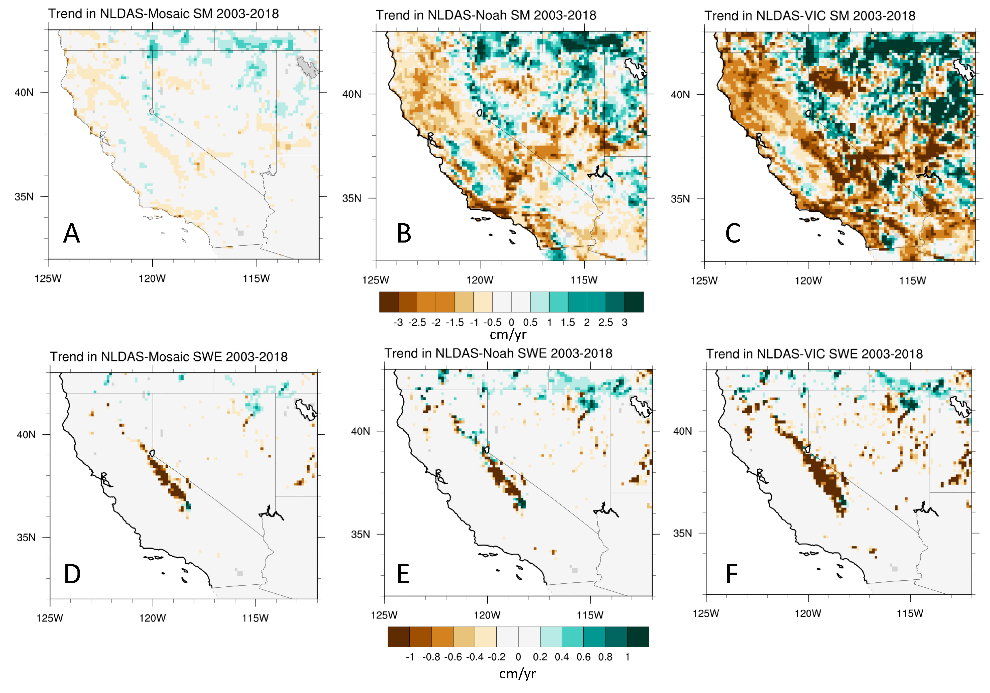
2.2. NLDAS—Mosaic, Noah, and VIC

The North American Land Data Assimilation System (NLDAS-2) constructs quality-controlled, and spatially and temporally consistent, land-surface model (LSM) datasets from the best available observations and model outputs [19,31] Data sets are available on hourly, daily, monthly and climatological time scales. NLDAS products are used in modeling, research, and applications, such as drought and flood monitoring, watershed and water quality management, and case studies of extreme events. NLDAS integrates a large quantity of observation-based and model reanalysis data to drive offline (not coupled to the atmosphere) land surface models (LSMs), and is executed at 1/8th-degree grid spacing over North America.
The models we use from NLDAS are the Noah, Mosaic, and VIC land surface models. We extract and use monthly average soil moisture at the 1 m level (SM) (Figure 2A−C) and snow water equivalent (SWE) (Figure 2D−F) outputs from each model for the years 2003–2018. The NLDAS-2 data used in this study can be downloaded at https://disc.gsfc.nasa.gov/datasets?keywords=NLDAS. Figure 2 shows temporal trends in SM and SWE for 2003–2018 simulated by the suite of NLDAS-2 models. As shown in Figure 2, there are large discrepancies between the various model simulations, which create uncertainties for our estimates of SM and SWE. We define the uncertainty for each process as the standard deviation (std) between the ensemble of three models at each time step (Figure 3B,C):
SWE (t) = std (SWENoah (t), SWEMosaic (t), SWEVIC (t))
SM (t) = std (SMNoah (t), SMMosaic (t), SMVIC (t))

2.3. Reservoir Data from the California DWR

The California Department of Water Resources (DWR) is a government agency that is responsible for managing and protecting California’s water. The DWR provides the California Data Exchange Center (CDEC), which installs, maintains, and operates an extensive hydrologic data collection network including data on the largest reservoirs in California, which we use in this study. The data can be downloaded at http://cdec.water.ca.gov/reservoir.html. We extract the information for the 50 largest reservoirs in California for the period 2003-2018, and use this as our Surface Water (SW) portion of the hydrologic cycle for this study. As done in previous studies (e.g., [7]), we apply 15% noise to the reservoir level data to obtain uncertainty estimates for surface water (Figure 3D), i.e., σSW (t) = 0.15 × (SW (t))

2.4. Data Processing to Calculate Groundwater

Each data product was re-gridded to match the GRACE product resolution (GRACE resolution = 0.50° × 0.50°). The original NLDAS simulations had a resolution = 0.125°, but these were re-gridded using bi-linear interpolation to match the gridding of the GRACE product. Once all products were on the same grid, we performed an area-weighted average that accounted for grid areas as a function of latitude. Then each of the data pieces was accumulated (summed) to obtain a temporal curve with uncertainties for each process (i.e., TWS(t), SM(t), and SWE(t)). The DWR reservoir data were in the form of point information, but we added up all these values to get one temporal data vector for California (i.e., SW(t)). Finally, once all the data was in the form of a temporal vector (with uncertainties), we were able to estimate the groundwater and its uncertainty.

2.5. Groundwater Estimates and Associated Uncertainties

The GRACE products estimate total mass change; therefore, the contributions of mass changes from other processes must be estimated before the groundwater mass change can be inferred [7]. Typically, this is done with a numerical land surface model. However, one standing issue with respect to GRACE is how much of the derived groundwater mass change is due to anthropogenic causes versus model error. Addressing this requires a rigorous and robust treatment of uncertainties that come with individual model corrections. Below, we outline the essential steps for deriving groundwater storage change and the approach we adopt to quantify the associated uncertainties.
The GRACE total water storage (TWS(t)) data were processed in a way that was able to quantify the uncertainty of the temporal dynamics of groundwater storage change aggregated for California (Figure 3A). We used information for soil moisture (SM(t)), snow (SWE(t)) and surface water (SW(t)) aggregated for the GRACE analysis region as described in Section 2.2 and Section 2.3, and then subtracted their effects from the TWS variations (TWS(t)) obtained from GRACE, where t indicates time. Our analysis was performed at monthly resolution. Therefore, the time-specific changes in groundwater (GW(t)) for a region are given by the following:
GW(t) = TWS(t) - [ SM(t) + SWE(t) + SW(t)] + ε (t)
We applied the Monte Carlo method and draw n = 1000 ensembles by introducing the uncertainty from each hydrologic process (i.e., TWS, SM, SWE, and SW). The calculation uses a normal (Gaussian) error with standard deviation σ, or N(0, σ):
ε (t) = N(0, σTWS(t)) + N(0, σSWE(t)) + N(0, σSM(t)) + N(0, σSW(t))
The uncertainty of TWS, or σTWS in Equation (4), is directly the error associated with the GRACE measurements, which is offered as part of the data product. The uncertainty information for SM and SWE, or σSM and σSWE in Equation (4), was obtained from the NLDAS-2 models. We characterized the uncertainty of SM and SWE as the standard deviation (std) between the ensemble of three models at each time step from the Mosaic, VIC, and Noah land surface models. The data for the reservoirs that represent the surface storage were obtained from the California Department of Water Resources (DWR). The uncertainty of the surface reservoir storage, or σSW in Equation (4), was assigned as 15% of the magnitude of the storage, a conservative approach that has been employed in previous studies (e.g., [7]).
After propagating all the sources of uncertainty, we were able to estimate the temporal groundwater dynamics for California with uncertainties (see Figure 3E). Note that there should theoretically be a correlation between the error components, since these processes are directly linked with one another. One way to account for this is to include these correlation terms (if they were known) in the non-diagonals of the error matrices. Although accounting for these correlations is beyond the scope of the current paper, we believe it could provide further insight on how these processes co-evolve together.

2.6. Wavelet Analysis

Many scientists have made use of the wavelet method in analyzing time series in geophysical or climate studies [39,40]. At present, there are many easy-to-use wavelet software packages for analyzing two time series together. Here, we used the cross wavelet transform and wavelet coherence (i.e., https://www.mathworks.com/matlabcentral/fileexchange/47985-cross-wavelet-and-wavelet-coherence) for examining relationships in the time frequency domain between two time series [40]. Grinstead et al. demonstrated how phase angle statistics can be used to gain confidence in causal relationships and test mechanistic models of physical relationships between time series. As hypothesized, the annual and year-to-year dynamics of the hydrologic cycle should portray a clear cascading effect. To investigate this further, we applied a wavelet analysis, which shows the frequency (in months) with which there is a clear signature between the temporal correlation of two processes. We applied this test to show the wavelet analysis results for each pair of processes estimated in our study.

3. Results

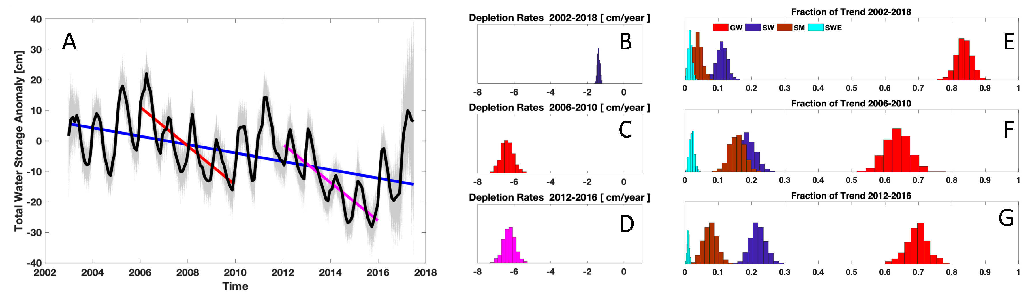
3.1. Trends in the Water Cycle

Figure 1 shows trends in TWS estimated by the GRACE products for different time periods, including two drought periods. A trend of roughly -2 (+/− 0.15) cm/yr is observed during the entire time period of our analysis (2002−2017). However, this trend has been up to -5 (+/− 0.65) cm/yr during drought periods (2006−2010 and 2012−2016). In Figure 2, trends in SM and SWE simulated by the NLDAS-2 suite of models are shown. For SM (Figure 2A−C), there are significant differences in the simulated trends between the various models, but losses of water from SM are estimated to have been roughly −1 (+/− 0.25) cm/yr, and as high as −3 cm/yr in some regions. For SWE (Figure 2D−F), most models agree that there has been roughly −1 (+/− 0.10) cm/yr loss of fresh water from the snow pack.
After applying the method described in Section 2.5, we are able to estimate the groundwater anomalies for the period of the study. Figure 3 shows the timeline of each hydrologic process, along with their respective uncertainty bounds. Table 1 reports the signal of water loss from each process, for different time periods. These numbers are also displayed in Figure 4, where the processes that contribute to the trends seen in TWS are disentangled and displayed separately. In summary, these results indicate that the majority of the loss in TWS is caused by groundwater depletion. This is especially apparent when we look at the volume of water lost in the right column of Table 1, where groundwater makes up the majority of this signal. Also, in Figure 4E−G, we show that groundwater makes up 60%−90% of the signal seen in TWS loss (red histograms).

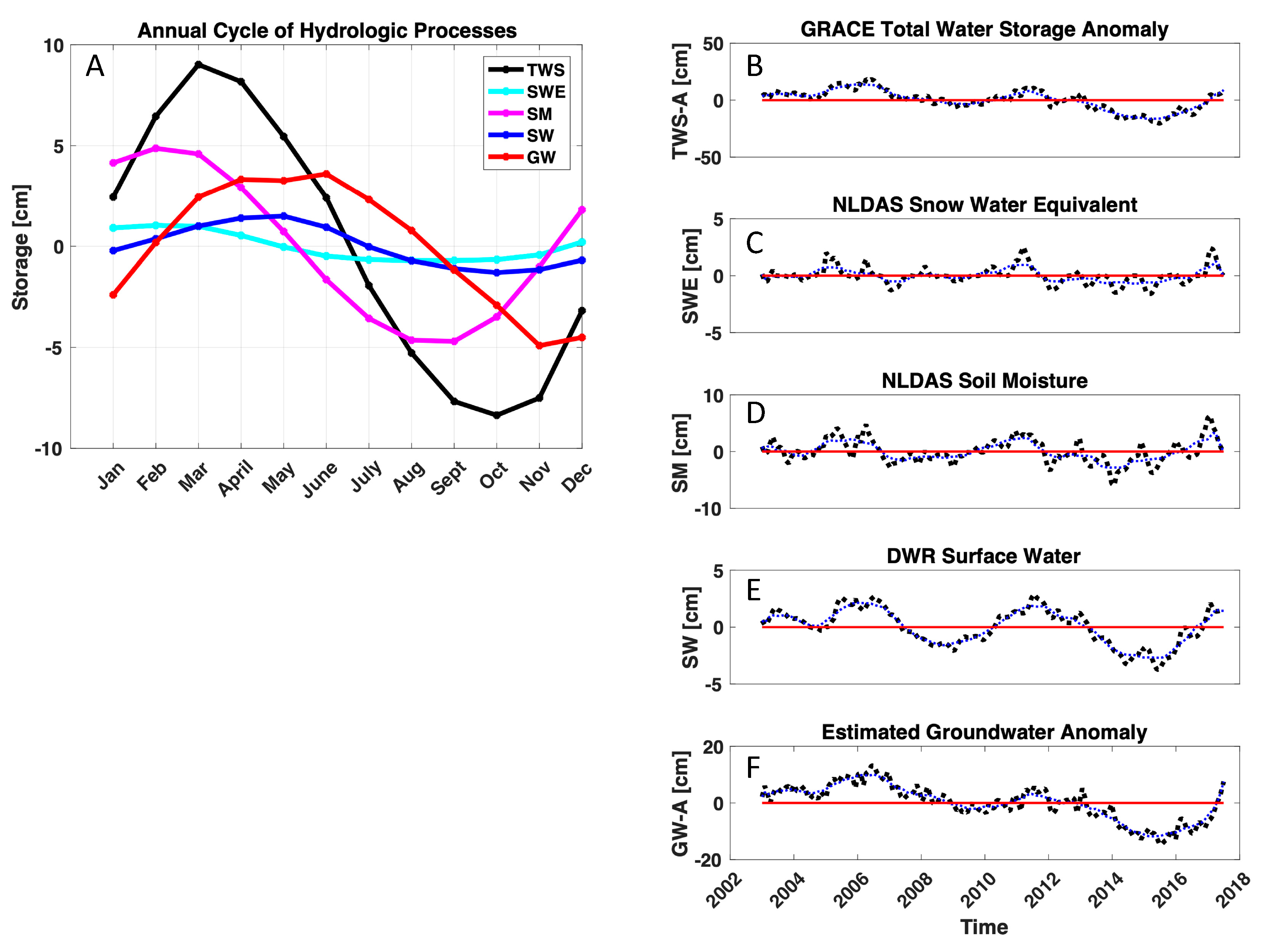
3.2. Cascading Effect of Hydrologic Cycle

In this section, we aim to capture the cascading nature of the hydrologic cycle. Figure 5A shows the mean annual cycle of the monthly averages for each process. We see that SWE and SM have peaks and also minimums that occur earlier than surface water and groundwater. For SWE and SM, the peaks occur around winter time, and the minimums around summer. For surface water and groundwater, the peaks occur around the spring, and the minimums occur in the fall. The cascading effect of the water cycle on an annual scale is therefore depicted here in these figures.
Figure 5B–F illustrates the de-seasonalized data, which we use to estimate the start, the peak, and the ending of the drought periods for each hydrologic process. This processing step is done to change the raw simulations into ones that show deviation from the annual cycle. In other words, if a certain process has a low or high value relative to the same month in the historic record, this processing step captures that deviation. This also allows us to investigate all of the processes as anomalies, which matches the forms of TWS and GW. These deviations, shown with black dots in Figure 5B–F, are computed by subtracting the mean annual cycle shown in Figure 5A from the mean simulations shown in Figure 3. A 13-month running mean (blue dots) show the state of each water process relative to its climatology for that month while smoothing out high-frequency fluctuations. This allows us to understand whether a certain process has low or high levels of water storage relative to its past states, and thus to quantify the timing of the beginning, peak, and ending of the drought for each process.
Our estimated start, peak, and ending of each drought period for each hydrologic process are displayed in Table 2. Also included are the peak magnitudes of volumetric water loss (in km3) for each component. These results indicate that snow and soil moisture are impacted earlier than surface water and groundwater. By initial inspection using the values in Table 2, we can estimate that there is a lag of roughly 8–16 months between the impact on SM and SWE compared to that of SW and GW. The next section highlights another way to quantify this temporal lag correlation between the various processes through wavelet analysis.

3.3. Results from the Wavelet Analysis

As mentioned in the previous section, the annual and year-to-year dynamics shown in our results portray a clear cascading effect of the hydrologic cycle on the scale of 8−16 months. To investigate this further, we apply a wavelet analysis which shows the frequency at which there is a clear signature between the temporal correlations of two processes. Figure 6 shows the wavelet analysis results for each pair of processes that we estimate in our study. The time series used for each process in the wavelet analysis shown in Figure 6 are the mean state estimates from Figure 3 (blue lines). We also applied this analysis on the 13-month running means from Figure 5B−F (blue dotted lines), but do not show the wavelet analysis for these time series since there were no coherent relationships between them. This is possibly due to the loss of information when applying a running average.
The panel on the top right of Figure 6 shows that, for TWS and groundwater, there is a high power signal (yellow colors), suggesting there is high correlation at around 8−16 months between these two processes. Outside of this time window, e.g., at 4 or 32 months, there is a low power signal (blue colors), which indicates there is little correlation between the two processes. the frequency of correlation at around 8−16 months is observed between all pairs of hydrologic processes. This indicates that the evolution of the hydrologic cycle occurs through an 8–16 month window. This window presumably begins with the rise and fall of soil moisture and snow pack in the winter and spring, followed by the decline of surface water and groundwater. These sources of water will continue to be relied upon and depleted in the summer time until the next season with sufficient rain begins, which could be the next or even the following Fall. This is what describes the pulse of roughly 8−16 months for the hydrologic cycle in California.
The correlation seen in the 8–16 month time range is a combination of both natural as well as human factors. First, the period of the annual rainfall accumulation affects other processes, like the accumulation of snow, soil moisture, and reservoir storage. Once the rainfall is finished for the year and the natural processes take their course, such as snow melting and soil moisture evaporation, the next step of this cascading evolution is the human use of water. By releasing reservoir storage and pumping groundwater to meet the demands of the human population, the final aspect of this cascading hydrologic cycle is complete as water reserves are depleted. The cycle starts again with the new rainfall of the next year. This roughly explains the 8–16 month window that is captured with the wavelet analysis, which is a result of both natural and human factors.

4. Summary and Discussion

In this study, we explored the temporal co-evolution of various aspects of the hydrologic cycle in California from 2002-2018. We combined information from the GRACE satellites, the NLDAS suite of models, and the California DWR to analyze dynamics of Total Water Storage, soil moisture, snow pack, large reservoirs, and finally, groundwater. We calculated groundwater after propagating uncertainties from other hydrologic processes and factored them out of the TWS estimates from GRACE.
There were clear trends of losses in water volume for all hydrologic processes. For TWS, a trend of -2 cm/yr was observed during the entire time period (Figure 1), and −5 cm/yr during drought periods (2006−2010 and 2012−2016). We disentangled the various processes from this trend, and found that the majority of the loss in TWS is caused by groundwater depletion (Figure 2 and Figure 4; Table 1). We quantified the start, the peak, and the ending of the drought periods for each hydrologic process, and showed that snow and soil moisture are impacted earlier than surface water and groundwater (Figure 5; Table 2). The annual and year-to-year dynamics shown in our results portray a clear cascading effect of the hydrologic cycle on the scale of 8−16 months (Figure 5 and Figure 6).
Overall, this study displayed the cascading evolution of the hydrologic cycle in California. This timeline begins with the accumulation of soil moisture and snow pack in the winter and its release in the spring, followed by the decline of surface water and groundwater during the drier summer period. Studies like this can help scientists and water managers better define and characterize droughts and their impacts. Generally, drought is defined by the lack of precipitation or the depletion of visible reserves such as reservoir storage or low snowpack. This study showcased the lagged effect of a drought, which also includes the depletion of groundwater reserves. It can be a mistake to assume the end of a drought period is reached as soon as rainfall occurs, since other aspects of the hydrologic cycle may not be replenished for months or years after. In this study, we hoped to portray that all aspects of the hydrologic cycle should be considered when characterizing a drought, and the cascading effect of this cycle can be confidently quantified, as we did here.

Author Contributions

Conceptualization, E.M., M.T., J.R., J.H., Z.L. and C.H.D.; Data curation, E.M., M.T., J.R.; Formal analysis, E.M., M.T., J.R., J.H. and C.H.D.; Funding acquisition, M.T.; Investigation, E.M., M.T. and J.R.; Methodology, E.M., M.T. and J.R.; Project administration, M.T. and C.H.D.; Resources, J.H.; Supervision, M.T.; Writing—original draft, E.M.; Writing—review & editing, J.R., J.H., Z.L. All authors have read and agreed to the published version of the manuscript.

Acknowledgments

The research was carried out at the Jet Propulsion Laboratory, California Institute of Technology, under a contract with the National Aeronautics and Space Administration (80NM0018D0004). Copyright 2020. All data used in this study are publicly available. The GRACE data set is available at https://grace.jpl.nasa.gov/data/get-data/, the NLDAS model output data are available at https://disc.gsfc.nasa.gov/datasets?keywords=NLDAS, and the DWR dats can be found at http://cdec.water.ca.gov/reservoir.html. The software package for wavelet analysis can be found at https://www.mathworks.com/matlabcentral/fileexchange/47985-cross-wavelet-and-wavelet-coherence.

Conflicts of Interest

The authors declare no conflict of interest.

References

  1. McCallum, A.M.; Andersen, M.S.; Giambastiani, B.M.; Kelly, B.F.; Ian Acworth, R. River–aquifer interactions in a semi-arid environment stressed by groundwater abstraction. Hydrol. Process. 2013, 27, 1072–1085. [Google Scholar] [CrossRef]
  2. Huang, J.P.; Ji, M.X.; Xie, Y.K.; Wang, S.S.; He, Y.L.; Ran, J.J. Global semi-arid climate change over last 60 years. Clim. Dyn. 2016, 46, 1131–1150. [Google Scholar] [CrossRef] [Green Version]
  3. Woodhouse, C.A.; Meko, D.M.; Macdonald, G.M.; Stahle, D.W.; Cook, E.R. A 1,200-year perspective of 21st century drought in southwestern North America. Proc. Natl. Acad. Sci. 2010, 107, 21283–21288. [Google Scholar] [CrossRef] [PubMed] [Green Version]
  4. McGuire, V. Water-Level Changes in the High Plains Aquifer, Predevelopment to 2007, 2005–06, and 2006–07; Scientific Investigations Report 2009-5019; U.S. Department of the Interior, U.S. Geological Survey: Reston, VA, USA, 2009.
  5. Rodell, M.; Velicogna, I.; Famiglietti, J.S. Satellite-based estimates of groundwater depletion in India. Nat. 2009, 460, 999–1002. [Google Scholar] [CrossRef] [Green Version]
  6. Wada, Y.; Van Beek, L.P.H.; Van Kempen, C.M.; Reckman, J.W.T.M.; Vasak, S.; Bierkens, M.F.P. Global depletion of groundwater resources. Geophys. Res. Lett. 2010, 37. [Google Scholar] [CrossRef] [Green Version]
  7. Famiglietti, J.S.; Lo, M.-H.; Ho, S.L.; Bethune, J.; Anderson, K.J.; Syed, T.H.; Swenson, S.C.; De Linage, C.R.; Rodell, M. Satellites measure recent rates of groundwater depletion in California’s Central Valley. Geophys. Res. Lett. 2011, 38. [Google Scholar] [CrossRef] [Green Version]
  8. Famiglietti, J.S. The global groundwater crisis. Nat. Clim. Chang. 2014, 4, 945–948. [Google Scholar] [CrossRef]
  9. Richey, A.S.; Thomas, B.F.; Lo, M.-H.; Reager, J.T.; Famiglietti, J.S.; Voss, K.; Swenson, S.; Rodell, M. Quantifying renewable groundwater stress with GRACE. Water Resour. Res. 2015, 51, 5217–5238. [Google Scholar] [CrossRef]
  10. Shang, H.; Wang, W.; Dai, Z.; Duan, L.; Zhao, Y.; Zhang, J. An ecology-oriented exploitation mode of groundwater resources in the northern Tianshan Mountains, China. J. Hydrol. 2016, 543, 386–394. [Google Scholar] [CrossRef]
  11. Massoud, E.C.; Purdy, A.J.; Miro, M.E.; Famiglietti, J.S. Projecting groundwater storage changes in California’s Central Valley. Sci. Rep. 2018, 8, 12917. [Google Scholar] [CrossRef]
  12. Liu, Z.; Liu, P.-W.; Massoud, E.; Farr, T.G.; Lundgren, P.; Famiglietti, J.S. Monitoring Groundwater Change in California’s Central Valley Using Sentinel-1 and GRACE Observations. Geosciences 2019, 9, 436. [Google Scholar] [CrossRef] [Green Version]
  13. Scanlon, B.R.; Longuevergne, L.; Long, D. Ground referencing GRACE satellite estimates of groundwater storage changes in the California Central Valley, US. Wat. Resour. Res. 2012, 48, W04520. [Google Scholar] [CrossRef] [Green Version]
  14. Harbaugh, A.W.; Banta, E.R.; Hill, M.C.; McDonald, M.G. MODFLOW-2000, The U.S. Geological Survey Modular Ground-Water Model-User Guide to Modularization Concepts and the Ground-Water Flow Process; Open-File Report 00-92; U.S. Geological Survey: Reston, VA, USA, 2000.
  15. Margulis, S.A.; Cortés, G.; Girotto, M.; Durand, M. A Landsat-era Sierra Nevada snow reanalysis (1985–2015). J. Hydrometeorol. 2016, 17, 1203–1221. [Google Scholar] [CrossRef]
  16. Yang, Z.-L.; Niu, G.-Y.; Mitchell, K.E.; Chen, F.; Ek, M.B.; Barlage, M.; Longuevergne, L.; Manning, K.; Niyogi, D.; Tewari, M.; et al. The community Noah land surface model with multiparameterization options (Noah-MP): 2. Evaluation over global river basins. J. Geophys. Res. Space Phys. 2011, 116, D12110. [Google Scholar] [CrossRef]
  17. He, X.; Wada, Y.; Wanders, N.; Sheffield, J. Intensification of hydrological drought in California by human water management. Geophys. Res. Lett. 2017, 44, 1777–1785. [Google Scholar] [CrossRef] [Green Version]
  18. Zaitchik, B.F.; Rodell, M.; Reichle, R.H. Assimilation of GRACE Terrestrial Water Storage Data into a Land Surface Model: Results for the Mississippi River Basin. J. Hydrometeorol. 2008, 9, 535–548. [Google Scholar] [CrossRef]
  19. Xia, Y.; Mitchell, K.; Ek, M.; Cosgrove, B.; Sheffield, J.; Luo, L.; Alonge, C.; Wei, H.; Meng, J.; Livneh, B.; et al. Continental-scale water and energy flux analysis and validation for North American Land Data Assimilation System project phase 2 (NLDAS-2): 2. Validation of model-simulated streamflow. J. Geophys. Res. 2012, 117, D03109. [Google Scholar] [CrossRef]
  20. Lo, M.-H.; Famiglietti, J.S. Irrigation in California’s central valley strengthens the southwestern us water cycle. Geophys. Res. Lett. 2013, 40, 301–306. [Google Scholar] [CrossRef] [Green Version]
  21. Faunt, C.C.; Hanson, R.; Belitz, K. Groundwater Availability of the Central Valley Aquifer, California; Professional Paper 1766; U.S. Geological Survey: Reston, VA, USA, 2009.
  22. Dong, L.; Wang, W.; Ma, M.; Kong, J.; Veroustraete, F. The change of land cover and land use and its impact factors in upriver key regions of the Yellow River. Int. J. Remote. Sens. 2009, 30, 1251–1265. [Google Scholar] [CrossRef]
  23. Siebert, S.; Burke, J.; Faures, J.M.; Frenken, K.; Hoogeveen, J.; Döll, P.; Portmann, F.T. Groundwater use for irrigation–a global inventory. Hydrol. Earth Syst. Sci. 2010, 14, 1863–1880. [Google Scholar] [CrossRef] [Green Version]
  24. Lund, J.; Medellin-Azuara, J.; Durand, J.; Stone, K. Lessons from California’s 2012–2016 drought. J. Water Resour. Plan. Manag. 2018, 144, 04018067. [Google Scholar] [CrossRef] [Green Version]
  25. Alley, W.M. Flow and Storage in Groundwater Systems. Science 2002, 296, 1985–1990. [Google Scholar] [CrossRef] [Green Version]
  26. Yeh, P.J.-F.; Swenson, S.C.; Famiglietti, J.S.; Rodell, M. Remote sensing of groundwater storage changes in Illinois using the Gravity Recovery and Climate Experiment (GRACE). Water Resour. Res. 2006, 42. [Google Scholar] [CrossRef]
  27. Purdy, A.J.; David, C.H.; Sikder, S.; Reager, J.T.; Chandanpurkar, H.A.; Jones, N.L.; Matin, M.A. An Open-Source Tool to Facilitate the Processing of GRACE Observations and GLDAS Outputs: An Evaluation in Bangladesh. Front. Environ. Sci. 2019, 7, 155. [Google Scholar] [CrossRef]
  28. Tapley, B.D.; Bettadpur, S.; Ries, J.C.; Thompson, P.F.; Watkins, M.M. GRACE Measurements of Mass Variability in the Earth System. Science 2004, 305, 503–505. [Google Scholar] [CrossRef] [Green Version]
  29. Reager, J.T.; Thomas, A.C.; Sproles, E.A.; Rodell, M.; Beaudoing, H.K.; Li, B.; Famiglietti, J.S. Assimilation of GRACE Terrestrial Water Storage Observations into a Land Surface Model for the Assessment of Regional Flood Potential. Remote. Sens. 2015, 7, 14663–14679. [Google Scholar] [CrossRef] [Green Version]
  30. Xiao, M.; Koppa, A.; Mekonnen, Z.; Pagán, B.R.; Zhan, S.; Cao, Q.; Aierken, A.; Lee, H.; Lettenmaier, D.P. How much groundwater did California’s Central Valley lose during the 2012– 2016 drought? Geophys. Res. Lett. 2017, 44, 4872–4879. [Google Scholar] [CrossRef]
  31. Mitchell, K.E.; Lohmann, D.; Houser, P.R.; Wood, E.F.; Schaake, J.C.; Robock, A.; Cosgrove, B.A.; Sheffield, J.; Duan, Q.; Luo, L.; et al. The multi-institution North American Land Data Assimilation System (NLDAS): Utilizing multiple GCIP products and partners in a continental distributed hydrological modeling system. J. Geophys. Res. Space Phys. 2004, 109. [Google Scholar] [CrossRef] [Green Version]
  32. Tiwari, V.M.; Wahr, J.; Swenson, S. Dwindling groundwater resources in northern India, from satellite gravity observations. Geophys. Res. Lett. 2009, 36, 18401. [Google Scholar] [CrossRef] [Green Version]
  33. Voss, K.A.; Famiglietti, J.S.; Lo, M.-H.; Linage, C.; Rodell, M.; Swenson, S.C. Groundwater depletion in the Middle East from GRACE with implications for transboundary water management in the Tigris-Euphrates-Western Iran region. Water Resour. Res. 2013, 49, 904–914. [Google Scholar] [CrossRef] [Green Version]
  34. Forootan, E.; Rietbroek, R.; Kusche, J.; Sharifi, M.; Awange, J.; Schmidt, M.; Omondi, P.; Famiglietti, J. Separation of large scale water storage patterns over Iran using GRACE, altimetry and hydrological data. Remote. Sens. Environ. 2014, 140, 580–595. [Google Scholar] [CrossRef] [Green Version]
  35. Moiwo, J.; Yang, Y.; Li, H.; Han, S.; Hu, Y. Comparison of GRACE with in situ hydrological measurement data shows storage depletion in Hai River basin, Northern China. Water SA 2009, 35, 663–670. [Google Scholar] [CrossRef] [Green Version]
  36. Feng, W.; Zhong, M.; Lemoine, J.M.; Biancale, R.; Hsu, H.T.; Xia, J. Evaluation of groundwater depletion in North China using the Gravity Recovery and Climate Experiment (GRACE) data and ground-based measurements. Water Resour. Res. 2013, 49, 2110–2118. [Google Scholar] [CrossRef]
  37. Watkins, M.M.; Wiese, D.N.; Yuan, D.-N.; Boening, C.; Landerer, F.W. Improved methods for observing Earth’s time variable mass distribution with GRACE using spherical cap mascons. J. Geophys. Res. Solid Earth 2015, 120, 2648–2671. [Google Scholar] [CrossRef]
  38. Wiese, D.N.; Yuan, D.-N.; Boening, C.; Landerer, F.W.; Watkins, M.M. JPL GRACE Mascon Ocean, Ice, and Hydrology Equivalent Water Height RL05M.1 CRI Filtered Version 2, PO.DAAC, CA, USA. Available online: http://dx.doi.org/10.5067/TEMSC-2LCR5 (accessed on 1 October 2018).
  39. Foufoula-Georgiou, E.; Kumar, P.; Mukerji, T.; Mavko, G. Wavelets in geophysics. Pure Appl. Geophys. 1995, 145, 374–375. [Google Scholar]
  40. Grinsted, A.; Moore, J.C.; Jevrejeva, S. Application of the cross wavelet transform and wavelet coherence to geophysical time series. Nonlinear Process. Geophys. 2004, 11, 561566. [Google Scholar] [CrossRef]
Figure 1. Trends in TWS observed by the GRACE satellites for (A) the entire time period of the study, (B) the drought period from 2006 to 2010, and (C) the drought period from 2012 to 2016.
Geosciences 10 00071 g001
Figure 2. Trends in soil moisture (SM) and snow water equivalent (SWE) simulated by the NLDAS suite of models. (A,D) The Mosaic model. (B,E) The Noah model. (C,F) The VIC model.
Geosciences 10 00071 g002
Figure 3. Temporal dynamics with uncertainties for all water processes in California that are investigated in this study, including (A) TWS from GRACE, (B) SWE from NLDAS, (C) soil moisture from NLDAS, (D) reservoir storage from DWR, and (E) estimated groundwater anomalies calculated in this study.
Geosciences 10 00071 g003
Figure 4. (A) Temporal dynamics of TWS from GRACE. The blue line represents the trend of TWS for the entire time period, and the red and magenta lines represent the trend during drought periods. (B–D) Histograms showing the magnitude and its uncertainty of the trends in TWS depicted in Panel A for all of the ensemble simulations. (E–G) Disentangling the trends in TWS shows that the majority of the losses are due to changes in groundwater storage (red), compared to losses in surface storage (blue), soil moisture (brown), or snow pack (light blue).
Geosciences 10 00071 g004
Figure 5. (A) The mean annual cycle for each process. The curves show the monthly averages. The cascading effect of the water cycle is clearly depicted in these figures. (B−F) Individual month deviations from the mean annual cycle (black dots), which shows each water process normalized by its interannual variability. A 13-month running mean (blue dots) show the state of each water process relative to its climatology for that month. This allows us to investigate the beginning, the peak, and the ending of each drought period.
Geosciences 10 00071 g005
Figure 6. Wavelet analysis showing the frequency at which there is a clear signature that the two plotted processes are correlated. For example, the panel on the top right shows that, for TWS and groundwater, there is a high power signal (yellow colors), which indicates there is high correlation at around 8-16 months. Outside of this time window, there is a low power signal (blue colors) which indicates there is little correlation between the two processes.
Geosciences 10 00071 g006
Table 1. Estimates of change in various components of the hydrologic cycle for the periods 2003−2017 (top), 2006−2010 (middle), and 2012−2016 (bottom). Total water storage is from the Gravity Recovery and Climate Experiment (GRACE), soil water and snow water storage are from model simulations (NLDAS), and surface water storage in the form of reservoirs is from the DWR. Estimates for groundwater storage are calculated in this study, and 1-sigma standard errors are shown for each estimate.
Entire Record2003−2017
Storage CompartmentTrend (cm/yr)Volume Trend (km3/yr)Volume Lost (km3)
Total−1.36 ± 0.15−3.98 ± 0.43−55.69
Soil Water−0.05 ± 0.04−0.15 ± 0.12−2.11
Snow Water−0.02 ± 0.02−0.06 ± 0.05−0.80
Reservoir−0.15 ± 0.04−0.44 ± 0.12−6.17
Groundwater−1.14 ± 0.16−3.33 ± 0.46−46.60
Drought 12006–2010
Storage CompartmentTrend (cm/yr)Volume Trend (km3/yr)Volume Lost (km3)
Total−6.37 ± 0.67−18.60 ± 1.97−74.40
Soil Water−1.00 ± 0.28−2.91 ± 0.81−11.64
Snow Water−0.13 ± 0.09−0.39 ± 0.27−1.55
Reservoir−1.19 ± 0.29−3.48 ± 0.85−13.92
Groundwater−4.05 ± 0.81−11.82 ± 2.36−47.29
Drought 22012−2016
Storage Compartment Trend (cm/yr)Volume Trend (km3/yr)Volume Lost (km3)
Total−6.28 ± 0.65−18.35 ± 1.89−73.41
Soil Water−0.49 ± 0.25−1.42 ± 0.72−5.70
Snow Water−0.06 ± 0.04−0.18 ± 0.12−0.72
Reservoir−1.37 ± 0.25 −4.00 ± 0.72−15.99
Groundwater−4.37 ± 0.74−12.75 ± 2.15−51.01
Table 2. Timing of the beginning, the peak, and the end of each drought period for each of the components of the hydrologic cycle. Also included are the peak magnitudes of water loss for each component during each drought (in km3).
2006−2010 DroughtSMSWESWGWTWS
Begin Drought 12006.82006.62007.52008.92008.4
Peak Drought 12007.42007.42008.72009.52009.5
End Drought 12009.72009.72010.32010.82010.4
Minimum (km3)−4.62−1.46−4.62−6.28−11.16
2012−2016 DroughtSMSWESWGWTWS
Begin Drought 22011.92011.82013.22012.92012.8
Peak Drought 220142014.72015.52015.22015.2
End Drought 22016.22016.62016.72017.32017.1
Minimum (km3)−8.30−2.02−7.89−34.73−48.23

