Abstract
A new method to solve thermal conjugacy problems is presented for layered models with a thermal conductivity jump at their boundaries. The purpose of this method is to approximate the inverse thermal conductivity coefficient, which has breaks, by using a combination of step functions. A generalized continuous operator is constructed in a continuous space of piecewise–homogeneous media. We obtained an analytical solution for the stationary problem of heat conjugacy in the layered model with finite thickness and with Dirichlet–Neumann conditions at the external boundaries. An algorithm was constructed for downward continuation of the heat flux to depths that correspond to the top of the mantle layer. The advantages of this method are illustrated by testing the crustal seismic, gravity and geothermal data of a study area in the Urals and neighboring regions of Russia. We examined statistical relations between density and thermal parameters and determined heat flux components for the crust and the mantle. The method enables a downward continuation of the heat flux to the base of the upper mantle and allows us to determine the thermal effects of the lateral and vertical features of deep tectonic structures.
1. Introduction
Heat flux is an important character of the thermal state of the lithosphere. It indicates conductive heat exchange in solid bodies and defines the direction of the evolution of deep tectonic processes. The use of geothermal data as a part of a complex interpretation scheme (along with gravity, magnetic or seismic data) lowers the ambiguity of geologic modeling and increases the reliability of the obtained models [1,2,3].
Heat flux is measured by temperature and its gradients at deep and ultra-deep parameter wells. These measurements have unique features. First of all, it is necessary to drill in order to obtain direct measurements, which significantly increases survey time and resources. In addition, a thermal equilibrium should be attained in the borehole, and the duration of this process may be up to several months [4]. The data obtained from the well are averaged, and then the analytic continuation of these heat flux values to the Earth’s surface is performed for all of the wells. The resulting values constitute the observed heat flux.
Obtaining a measured data set is very difficult because it is only possible to perform surveys of thermally stabilized wells. Thus, any three-dimensional (3D) model is an interpolation of several one-dimensional (1D) data sets, which are measured in such wells. This is why many researchers tend to utilize data obtained by other geophysical methods (such as seismic and gravity data) for thermal model construction [2,3]. One-dimensional measurements do not allow for the detailed study of structural features of a geothermal 3D model. However, the use of gravity field data along with thermal data allows us to control the density values of the model. This is especially important at the lower crust and upper mantle, where thermal parameter amplitudes are quite high and the corresponding heat flux anomalies can vary widely [2].
Geothermal models of the lithosphere should be enclosed by boundary conditions. The upper boundary Dirichlet condition corresponds to the constant temperature in the neutral layer. The lower boundary condition may be either the Dirichlet problem for temperature or the mixed Dirichlet–Neumann problem for heat flux. The Dirichlet problem is used when the boundary condition is defined by the temperature of solidus of basalts [5]. The thickness of the thermal lithosphere (around 200–300 km) is proportional to the value of the observed heat flux at the earth’s surface level and correlates with the age of the tectonic features [5]. The more flexible lower boundary value problem condition is the Neumann condition on heat flux [6]. Usually, it is specified on a Mohorovicic discontinuity surface [7,8] or at a mantle sole [9]. The upper mantle, which is located between Moho and approximately 80 km, has a block structure [10]. The heat flux from the mantle acts as an unknown boundary parameter of the forward geothermal problem. By changing this parameter, one can achieve the required level of match between the observed and calculated values of heat flux at the earth’s surface [9].
The stationary component of the thermal field is produced by the inner heat sources and deep (external) flux in the inhomogeneous lithosphere. More accurately, it should be called “quasi-stationary”, because radiogenic heat production is not constant over time. However, these changes are very slow. The stationary component should firstly be studied when we interpret regional anomalies and construct geothermal models [11].
Two factors contribute to the conductive thermal flux that is observed on the earth’s surface. The first one is the summary power of radiogenic heat production in the earth’s crust per unit squared. The second one generalizes deep heat loss inside the earth by setting a boundary condition on the mantle heat flux [6,8,9]. The stationary nature of the subsurface flux is defined by decay heat from long-lived isotopes of U238, Th232 and K40 in the earth’s crust. Half-lives of these elements are in the range of 1.3 to 12 billion years, so their order of magnitude is equal to the earth’s age [7,9]. The stationary nature of deep flux is only hypothesized. For example, if a single thermal impulse occurs in a layer at depth H below the earth’s surface, after the relaxation time (Fourier time interval) this non-stationary impulse will decay almost completely [12]. For the lithosphere layer of thickness H with thermal diffusivity cm2/s, the relaxation time can be evaluated by formula , where H is given in kilometers and in years. As we can see, the relaxation time of the deep heat flux perturbations is quite sensitive to the layer thickness. For the layer with H of 80 km, the relaxation time will be not less than 50 million years (Cenozoic Era), while for the layer with H in the range of 200 to 300 km, it will span over 0.3 to 0.7 billion years (Paleozoic Era). In our scheme, we assume that the stationarity of the thermal conditions prevails for the heat flux from a level of 80 km. We only study conductive heat flux in solid bodies; this is why we do not consider the influence of thermal convection [13].
Under certain conditions, boundary value problems involving steady state thermal fields may be considered as belonging to a specific type of potential. In cases where the basal heat flux is small, only two physical parameters are taken into account: the power of radiogenic heat generation sources (Q), and the thermal conductivity coefficient (λ). However, the distribution of thermal flux becomes inhomogeneous when heat transfer in the medium is controlled by a thermal conductivity contrast parameter. Heat flux from the mantle may be considered a deep boundary condition.
Temperature, T, as a potential function, satisfies the Poisson equation with a special type of volume and surface heat sources. In the case of constant thermal conductivity, the inhomogeneous distribution of heat sources, Q, does not introduce any serious difficulty to solving thermal problems, because they are algorithmically similar to known problems of gravity potential associated with mass density 4πQ/λ [14,15]. The solution to such problems, designated here as the gravithermal type, is of the volume Poisson integral type and can be calculated numerically. This is one of the reasons why gravithermal models are widespread in theoretical and practical geophysical research [5].
In the case of non-homogeneous thermal conductivity, a refracted component of the thermal flow appears, and the heat is transferred along the path of least thermal resistance. In piecewise–homogeneous models, abrupt changes in thermal conductivity are allowed. The normal component of the temperature gradient at a thermal contact boundary also undergoes abrupt changes. The contact boundary of media with different thermal conductivity values is the place of material discontinuity. A break in normal temperature gradients forms the equivalent simple layer of inducted sources [15,16].
A determination of heat transfers across this simple layer is obtained from boundary conditions of the thermal conjugacy (conditions of the fourth order). The problems of thermal conjugacy may only be solved by numerical methods using a conservative difference scheme for keeping the energy balance for every discrete element [14]. This problem is algorithmically difficult and requires a significant amount of resources, even for two-dimensional cases [8,9].
We developed a new analytical method for the thermal conjugacy formulation as a boundary value problem for the potential fields, which utilize the similarity in interpretation schemes of steady state thermal and gravity fields. Its main idea was presented earlier in [13], while in the current paper we provide a complete theoretical framework of the method. Following this, we construct an algorithm for its numerical solution, which is similar to the methods employed in calculations of gravity anomalies. These results are presented in the Methods section of the current work. In the Case Study section, we test it on a three-dimensional density distribution model, which was developed earlier [17]. The problem domain extends to 80 km, which is the first regional level of the isostatic compensation. Using statistical correlation of density versus heat production and density versus thermal conductivity, we build an earth’s crust and upper mantle model to solve the forward geothermal problem for density distributions given on a three-dimensional grid. Contribution of a deep thermal flux is evaluated by the method of analytical continuation to the Moho discontinuity.
2. Methods
The boundary value problem for the stationary heat conductivity in piecewise–homogeneous models is defined by second order differential equations. They have a strong break when the required constrains on the continuity of first derivatives are not satisfied in a space of solutions [14,16]. The contact boundaries of the neighbor media are the surfaces where the thermal conductivity coefficient has a break and, thus, a temperature gradient breaks too. Their functions have no value at these surfaces; however, the left side and right side limits exist. Such problems belong to a class of linear conjugacy with the implicitly defined boundary values (boundary conditions of the fourth kind), which are equal to the conditions of continuity of temperature and normal components of the heat flux in a 2-sided neighborhood of an ideal thermal contact [12].
In the space of generalized functions (i.e., in the linear space of continuous functionals), it is possible to avoid the construction of partial solutions for every homogeneous area and its subsequent stitching on the boundaries. A singular generalized continuous operator for an arbitrary point of the inhomogeneous space can be obtained both for the areas of continuity and the break boundaries.
The method for constructing an analytical solution to the conjugation problem in the space of generalized functions was briefly described in [13]. In Section 2.1, Section 2.2, Section 2.3 and Section 2.4 (with additions in Appendix A and Appendix B), we present it in a complete form.
2.1. Generalized Continuous Operator of the Conjugacy Problem
The models of stationary thermal fields include a distribution of two parameters: the strength of radiogenic heat generation sources , and the thermal conductivity . They are connected with an energy balance condition, namely summary flow through the closed surface S, which limits the area , is equal to a summary strength of the heat sources inside this area [12]:
or the same in a differential form is as follows:
For the non-homogeneously heated body, in which the temperature gradient is not large, the heat flow is proportional to the first degree of the temperature gradient [12]. This is Fourier’s law of heat conduction, which characterizes a conductive (or molecular) mechanism of heat transfer in a stationary media from areas with higher temperature to areas with lower temperatures. For isotropic bodies, the heat flow vector q points oppositely to the temperature gradient vector as follows:
The temperature refers to the “spreading” potential of the temperature gradients vector field (or the heat flux field). If the thermal conductivity λ is constant, the formula for the temperature matches the representation for the gravity potential with the equivalent mass density [14,15]. If the thermal conductivity is not constant, then the refracted component is added to the field of sources. At last, if the has an abrupt change on some boundary, then the temperature gradient component will change in the same direction. The flow (more accurate, its normal component) is continuous on the boundary; however, every function in production has a first order continuity break. In the neighborhood of such discontinuities, the boundary derivatives are replaced by the integral conditions of thermal conjugation [12].
A correctness of the continuous formulation of the conjugacy problem is ensured by a step approximation of the inverse thermal conductivity function in the area of the break surface. We can expand the operator definition area in Equations (2) and (3) by expressing its coefficients in terms of a valid combination of the inverse thermal conductivity break functions and its gradient as follows:
Here the production of one break function (the inverse thermal conductivity and its gradient) and the continuous density function of sources and the normal component of the flux exist as a valid functional combination [16,18]. Equation (2) is true not only at the points of continuity, but also at the inverse thermal conductivity coefficient break points. It corresponds to the continuous formulation of the conjugacy problem without boundary conditions.
Consider the layered media D with a flat top boundary at the earth’s surface and a flat bottom boundary (Figure 1). Inner boundaries separate D to (M + 1) curvilinear layers . Above the boundary, the thermal conductivity of the layer is constant and equal to ; the density of sources is continuous or at least integrable.
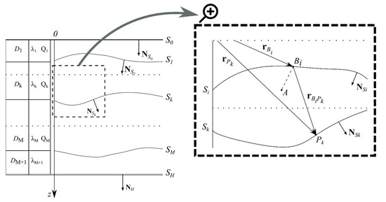
Figure 1.
Layered media model of thermophysical parameter distribution in lower semispace. A fragment of layers is shown on the right; position vectors are shown for the boundary points.
Let be the Cartesian coordinate system. The vertical axis is directed downwards, and the plane acts as the top boundary . The inner boundaries are defined implicitly by the function . Let denote a unit normal vector for the surface . The vector is proportional to the gradient , and downward normal direction is selected (Figure 1).
Now we introduce Heaviside step functions . The linear combination of these step functions forms the heuristic relation of a discontinuous coefficient of the inverse thermal conductivity versus coordinates of the media.
The generalized derivative of is equal to the Dirac delta function , which is supported on the surface , and, thus, [18]. Therefore,
The gradient member in Equation (4) can be converted into a form of simple layer sources as follows:
A surface density of the sources is equal to the jump of normal components of the temperature gradient.
Since the heat flow is continuous,
Here, is a value of the temperature derivative, which is equal to the half sum of limit values from both sides; is the thermal conductivity contrast between k-th and (k + 1)-th neighbor layers.
The transformed differential operator in Equation (7) is defined in break points of the thermal conductivity coefficient. Thus, as continuous functional in the generalized integral images space, it corresponds to a continual definition of the thermal coupling problem without boundary conditions.
2.2. Integral Transforms and Green’s Formula
Merging of a finite number of layers with different thermal conductivity values forms the geothermal model of layered media with flat boundaries and , as shown in Figure 1. Since the thermal coupling condition on M internal curvilinear boundaries is already included in the generalized continuous operator of the differential Equation (7), the solution should satisfy the bounding conditions only on the outer boundaries of the media. The stationary nature of the model is defined by the mixed Dirichlet–Neumann conditions [12,15]. The upper Dirichlet condition on the temperature corresponds to a isothermal mode on , while the lower Neumann condition on indirectly takes into account the heat flow on the boundary between the crust and the mantle.
Here is the constant temperature on the upper boundary of the medium; is the heat field strength at the lower boundary. It is assumed that the top and the bottom boundaries cross in infinitely remote points, making the area closed as follows: .
Integral image spaces of the boundary value problem (Equations (7)–(9)) is created by the convolution of the temperature Laplacian and the Green’s function , which is a singular function of two variables of a homogeneous boundary value problem [12,14] as follows:
Such a transform of the implicit kernel convolution (Equation (10)) is included in Green’s second identity as follows:
Note that the volume integral with the surface delta functions can be transformed into a sum of two-dimensional integral forms [18] of all the internal boundaries as follows:
Now we select the components from Green’s formula, which correspond to the two types of heat flow field sources. Contribution from the internal (i.e., located inside the volume) sources and the external sources (i.e., located on the lowest plane ) can be combined into a sum of the temperatures, which are not distorted by the thermal conductivity contrast.
These temperatures may be considered as primary potentials. The surface simple layer sources, which are created in the primary field on the inner boundaries , form the secondary potential:
The kernel of the integral operator defined by Equations (11) and (12) is Green’s function G, a known solution of a simpler boundary value problem (Equation (10)) under Dirichlet and Neumann homogeneous conditions [15]. This ensures a uniqueness of the solution if the energy balance (Equation (1)) is kept for the layered media. The difference between the integral flows on top and bottom boundaries is equal to the summary power of the inner heat sources inside the closed area , as follows:
2.3. Low Contrast Approximation
Equation (12) for the inhomogeneous boundary problem defined by Equations (7)–(9) is a convolution of the density of the simple layer sources with Green’s function. Such a form of equations allows one to separate mixed boundary conditions for the layered media model. Homogeneous Dirichlet and Neumann conditions on the external boundaries and are included into Green’s function . Conditions of the thermal conjugation on the inner boundaries define the surface density of the simple layer . Normal surface derivatives of Equation (12) can be substituted into a system defined by Equation (8) as follows:
Here, is a projection of an observation point A by normal to all boundaries ; (see Figure 1).
Let low contrast media be defined as the media with a jump in the thermal conductivity on each less than 2 times ( or ). In this case the in Equation (8) is small ( and the integral equations system can be replaced with a linear approximation as follows:
The contributions from internal and external thermal sources into the primary potential field (Equation (11) are separated. In the secondary potential they are separated as well. Substitution of the density value (Equation (15)) to the integral formula of the intermediate solution (Equation (12)) for the temperature leads us to the following formula:
This substitution does not change the additive structure of the operator (16). However, the kernel was changed as follows:
The superposition of Green’s functions (Equation (17)) takes into account not only the homogeneous Dirichlet and Neumann conditions, but also the heat flow refraction on its internal boundaries. Thus, the kernel is a full analogue for Green’s function for the layered media and the flat external boundaries.
2.4. Mantle Heat Flow
The uprising component of the heat flow at the boundary points opposite to the z axis, which means that its sign matches the sign of the temperature gradient.
On the earth’s surface the heat flow can be seen as a sum of the crustal radiogenic heat sources Q and the sources μ on the roof of the mantle layer :
Considering , we obtain an integral equation for the mantle component of the heat flow.
This integral equation allows one to solve the problem of a field continuation through the inhomogeneous (by thermal conductivity) media from the earth’s surface level to the depth . For the upward continuation of the mantle field component to the curvilinear boundary we have
Formulas (21) and (22) allow one to exclude the thermal field strength from the foot of the mantle layer. After this, the heat flow on the roof of the upper mantle can be represented through its value at the earth’s surface level.
3. Case Study
3.1. Initial Data
Now we demonstrate the method using a practical example. Our study area is the Urals and the neighbor regions of Russia, which are located at 60–68° N and 48–72° E. This is the near-Arctic zone of an important Russian geological provinces junction: the northeastern part of the East-European platform, the Timan-Pechora plate, the northern part of the Ural Folding System and the northwestern sector of Western Siberia. Seismic survey data were used for the construction of the build frame of a 3D density model [17]. These seismic (deep seismic sounding (DSS)) velocity profiles are shown in Figure 2a, while their geographic positions compared with a map of tectonic structures [19] are presented in Figure 2b.
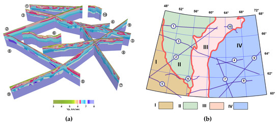
Figure 2.
Initial deep seismic sounding (DSS) profiles (a) and elements of the tectonic scheme of the region (by E.E. Milanovskiy [20]) (b). Red–white lines show generalized tectonic boundaries. Blue–white lines on (b) show the position of DSS profiles: Agat-2 (1), Globus (2), Quartz (3), V. Nildino–Kazym (4), Rubin-1 (5), Syktyvkarsk (6), N. Sosva–Yalutorovsk (7), Krasnolelinsk (8), Granit–Rubin-2 (9), Polar–Urals transect (10). Tectonic structures: Eastern European platform (I); Timan–Pechora plate (II); Urals Folding System (III); Western Siberian plate (IV).
The anomalies of the gravity field were reduced to the quasigeoid surface on a 2′ × 2′ grid [21,22]. A near-surface thermal flux was calculated from the temperature and thermal conductivity measurements in deep trial wells on a sparse network. This is the observed (measured) flux at the earth’s surface. At this resolution the unique features of the region, such as the Urals geosyncline [23], may be seen. These features are invisible in known global databases of the observed heat flux values [24,25], which have a resolution no more than 2° × 2°. Additionally we used geothermal survey data from the Urals–Siberian region [8,26], which were interpolated from the resolution 0.5° × 0.2° (lon × lat). The data on the eastern edge of the European platform and the Timan–Pechora plate were refined using earlier publications [7,9,11,27,28]. The resulting map is provided with the current paper in the Supplementary Materials. Data of gravity and thermal measurements were recalculated to a regular grid in zone 11 of a Gauss–Kruger projection [29,30]. Figure 3a presents the anomaly gravity field for our study area on a dense 1 × 1 km2 grid, which we also use for our density model. It is compared with the thermal flux on a sparse network of 10 × 10 km2, as seen in Figure 3b.
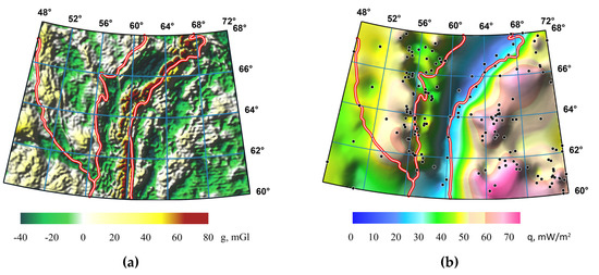
Figure 3.
Gravity anomaly field (a) and heat flow map (b) of our study region. Red–white lines show the position of generalized tectonic boundaries of the Urals Folding Belt and its neighboring platforms. Black dots show the position of wells.
The main Ural fault crosses the eastern side of the Urals at approximately 60 °E. It forms the western edge of the Urals geosyncline, which is the Hercynian tectonic fold. This zone has anomalous low heat flux values [23]. It corresponds to the regional maximum of the gravity field. The similarities in morphology are traced in other tectonic zones as well. However, there is no close connection between gravity and thermal anomalies. A correlation coefficient between these maps is only −0.31, while a correlation coefficient between the relief grid and the thermal flux grid is 0.76.
3.2. Initial Density Model
Two dimensional velocity data were obtained by profile sections from 10 deep seismic sounding (DSS) profiles. Velocity cuts down to Mohorovicic discontinuity were constructed using a method of seismic tomography. Below the Mohorovicic discontinuity, there is an upper mantle, which was constructed using an isostatic compensation method and has a block structure. The blocks were selected by residual anomalies of the gravity field and then were refined by the lithostatic pressure anomaly on the 80 km depth level. This 80 km depth is the first regional level of the isostatic compensation for the Urals [17].
Velocity data were recalculated to the densities using a known piecewise–linear regression function [31]. The gravity data can be used to connect the model density with the observed gravity anomalies. The regression coefficients were clarified during the inverse linear problem solution for all the velocity profiles of the region. Thus, we obtained a possible density analogue for the velocity model for deep structures.
Density profiles were bound to a three-dimensional grid (Figure 4a). They form a carcass of a density model. The vertical resolution of the model is 100 m, so it contains 800 layers between 0 and 80 km. The horizontal step of the discretization is 1 km by 1 km. The profile data were interpolated in each layer to fill the gaps between the profiles. The average density value was calculated for every layer. This set of density values forms the background density function of the model, which depends on depth only. Figure 4b shows along with minimal and maximal density values in the layers. As it can be seen, the average density mostly repeats the character of the minimal and maximal values. There is a sharp rise of the density at around 5–8 km below the earth’s surface (the sediment cover); at middle and lower crust depths, the gradient of the density change is low, and at 40–50 km there is a clearly visible step where the mantle blocks start to appear.
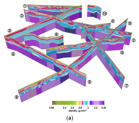
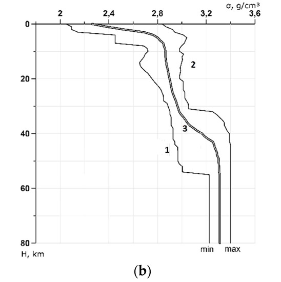
Figure 4.
Two-dimensional density values along 10 seismic profiles, which form the 3D carcass of the initial model: (a) the density profiles constructed by seismic data; (b) the dependency of minimum (1) and maximum (2) density values versus depth z; (3) the average density values on the corresponding depth levels.
3.3. Refined Density Model
The method of gravity inversion was developed by the authors and was described in [32]. The inversion was performed in layers consequentially; during this process, the model was refined to satisfy the observed field. The constructed 1D background density was used for the mass continuation outside the study volume. An absolute density value in every grid element was replaced with the density jump (excess density), which is relative to the background density. The iterative scheme of corrective additions calculations in the horizontal layers provides uniqueness of the inverse problem solution [33]. The resulting density model is presented in Figure 5. It consists of 1336 × 969 × 800 prismatic elements.
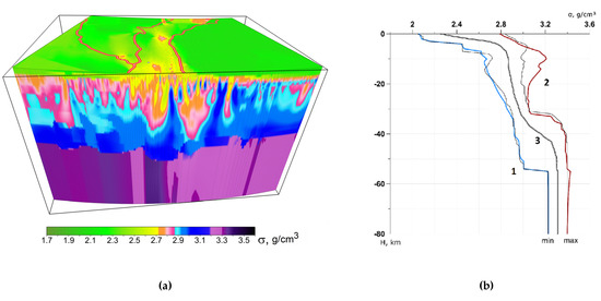
Figure 5.
Resulting density model (a) and its average density versus depth dependency (b). Here 1 is the minimum density value on the corresponding depth level, 2 is the maximum density value and 3 is the average density value. Thin black lines show dependency for the initial model for comparison.
The comparison of the initial distribution of minimum and maximum density values versus depth (Figure 4b) with the resulting one (Figure 5b) shows that there were almost no corrections made to the model in the lower crust and upper mantle. Therefore, the morphology of deeper boundaries (e.g., Moho), which was estimated by seismic data [3,34], cannot be refined in the process of gravity modeling.
3.4. Grid Approximation of Thermal Physical Parameters of Geothermal Model
Petrophysics surveys evaluate the dependency between rock densities and their heat production and thermal conductivity [5,6,8,9,11]. For igneous rocks, the dependency of the density values versus heat production is most visible and was estimated by Rybach [35,36]. For sedimentary and metamorphic rocks, the dependency for the concrete region should be used [2,8,27]. Usually it is in the form of heat production variation intervals for specified density values (e.g., [5,7]). Bulashevich performed a generalization of these dependencies for the Urals region [23] (Figure 6b). It is satisfactory because for acidic to ultra-alkaline rocks, the minimum and maximum values of the heat production variation intervals are close. Using this density versus heat production dependency, the 3D density model was recalculated into a corresponding thermal model of inner sources of the radiogenic heat production field. Figure 6a presents this 3D distribution of the crustal field sources.
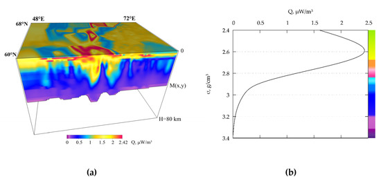
Figure 6.
Heat production model. Three-dimensional model of thermal sources in the earth’s crust above the Moho (a); generalized dependency between rock density and its thermal production for the region [23] (b).
Another important parameter of stationary thermal models is the thermal conductivity λ. Unfortunately, there is no stable and clearly visible relation between the thermal conductivity and the rock density. This happens because, in the first place, thermal conductivity depends on temperature and pressure, which partially compensate each another [23]. In addition, it depends on structural tectonic factors such as a geological age and type of stratification [5,6,9,11,37]. At this stage of research, we used values of thermal conductivity taken from a collection of rocks examples for the Urals and Siberian regions obtained by Duchkov et al. [26] and Golovanova [8]. This dependency, which takes the structural tectonic factors into account, is shown in Figure 7b.
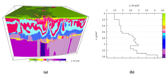
Figure 7.
Thermal conductivity distribution for elements of 3D density model of the earth’s crust and upper mantle (a); dependency between thermal conductivity λ and model density σ values (b).
3.5. Forward Geothermal Problem
The formulas for the stationary temperatures and heat flux for three-dimensional geothermal models of such a layered media were obtained for the condition of low contrast thermal conductivity [7,9,11]. Under this condition the calculated gravity and thermal fields are additive. This fact is the basis of our complex interpretation method for gravity and geothermal fields in inhomogeneous media. The calculation schemes for the heat flux (Equations (19)–(20)) and field continuation (Equations (21)–(22)) were implemented using the field grid step of 10 × 10 km2.
4. Results
Three dimensional distributions of the heat production sources in the earth’s crust and thermal conductivity λ in crust and mantle in the form of a 3D array are shown in Figure 6 and Figure 7 correspondingly. The heat flux field was calculated from these data using Equation (19). The component of Equation (19) was precalculated by an elementwise division of array (Figure 6a) by array (Figure 7a). The corrections for the thermal conductivity contrast from the simple layer sources were calculated for the model of two boundaries, and, thus, three layers [34]: a sediments layer with low thermal conductivity , and crustal and mantle layers with high thermal conductivity . Green’s function for the two flat boundaries (Equation (A10), Appendix A) and the function for the layered media (Equation (A17), Appendix B) correspond to the function of inverse distances in the gravity problem. Figure 8 presents the solution of the forward thermal flux calculation for the model using Equations (19) and (20). The heat flux for the earth’s crust is calculated at the earth’s surface level . The mantle component of the flow (Equation (20)) is calculated from the difference between the observed and calculated values of the heat flow.
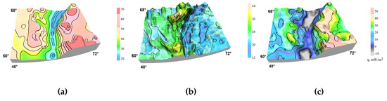
Figure 8.
Forward geothermal problem. The observed heat flux (a); the calculated heat flux values for the crust and sedimentary cover at level z = 0 (b); mantle component of heat flux (difference between (a) and (b)) at level z = 0 (c).
The mantle component of the flux at the upper boundary of the mantle is changing in wide interval from the normal (average) values of 20–30 mW/m2 at shields and ancient platforms (e.g., Eastern European platform and Timan Pechora plate) [2,5,27]; to high values of 40–50 mW/m2 and more at the western end of the young Western Siberian plate [11,37]. The mantle flux at the Urals is partially negative. On the one hand this is connected to the extremely low values of the measured temperature gradients and, thus, the calculated heat flux, in wells of the Urals geosyncline [8,23]. On the other hand, the relatively high thermal production at the mountain roots of the Urals Folding System may be the reason [9]. The negative values of stationary thermal flux at the earth’s surface level are against the physics of geothermal processes and require a reasonable adjustment of measured data taking the paleoclimate into account [38,39].
Inverse Problem of Analytical Fields Continuation
A deep heat flux, which is given through the Neumann boundary problem (Equation (9)), is a component of the solution of the forward problem for the temperatures (Equation (16)) and heat flux (Equation (20)). However, it is not an a priori known function. Nevertheless, a “trace” of this function can be clearly seen in the field flux difference (observed minus radiogenic) at the upper boundary z = 0 (Figure 8c). The lower bounding surface z = H is a helpful carrier of simple field sources with a density of . Thus, the right hand part of Equation (21) is a convolutional integral operator for a direct recalculation of the field from the level to the level . An inversion of the operator of Equation (21) gives us the solution of the inverse problem of the analytical continuation of the mantle component of the heat flux down through layered inhomogeneous media in the direction of field sources.
The inverse problem of the fields continuation is unstable with respect to irregular noise in the input data. This is why the algorithm for the analytical continuation should include a regularization parameter. Its value is selected that way so the continuation of the regularized solution to the initial height level matches (with some error) the initial field. The uprising heat flux at the upper isothermal surface has a vertical component only. The heat component of earth crust sources is excluded, and the remaining mantle component is recalculated to a vertical gradient of temperature at the lower bounding surface z = H. This is enough for the ability to correct geothermal parameters of boundary function and calculation of the temperature and heat flux vector components at every point of the layered inhomogeneous media.
To match the deep mantle component of heat flux with the relief of the upper mantle roof, the components of the temperature gradient vector were calculated as well as the uprising heat flux (Equation (22)) at the depths, which correspond to the Mohorovicic boundary position M (x,y). Figure 9 presents the results of the vertical component of mantle flux recalculation to the curvilinear surface of M boundary. The morphology of the recalculated fields repeats, in general, the relief of mantle structures, and they have a good match each with the other. The correlation coefficient between the mantle relief grid and thermal flux grid is 0.76, which was calculated by 133 × 97 grid elements on field grid.
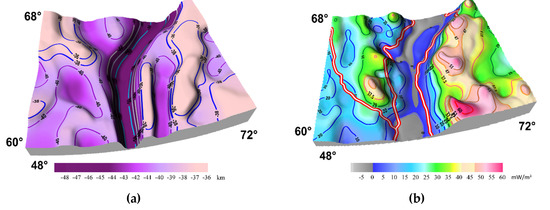
Figure 9.
Mantle thermal flux. Mohorovicic boundary M relief (a); deep component of the flux, which was recalculated to the roof of upper mantle (b). Double red–white line shows major tectonic structures.
The increased heat flux corresponds to the uplift (an increase in elevation) of Moho on the west side of the Western-Siberian plate [37], while the low flux values correspond to the boundary depression along the Urals mountain belt (approximately 59° E) and neighbor foreland basins [9]. On the contrary to these anomalous geothermal regions, the mantle flux at the eastern edge of the Eastern European platform and northern part of the Timan–Pechora plate is close to its background average values. This is usual for ancient shields and platforms [7,11,27].
The heat flux and the vertical component of the calculated temperature gradient at Moho (Figure 9b) correlates with the age of the geological structures of the earth’s crust as well as with the seismic waves velocity change at the Mohorovicic discontinuity [5,7]. Such a velocity inhomogeneity must be accompanied with inhomogeneous temperature distribution [10,36]. The lower the seismic waves velocity along the mantle boundary M is, the higher the temperature values of the mantle blocks [2,3,11,37].
An isostasy, which has been taken into account in the mathematic model, the change of the density value is controlled. The blocks in the model of the mantle in Figure 4 were selected taking the isostatic compensation hypothesis into account. The density of mantle blocks depends on the Moho boundary relief. Uplifts in the Moho correspond to the increase in thickness of the isostatic compensation layer and the decrease of the density (and the velocity) in a mantle block. The converse is also true; a decreased Moho relief corresponds to increased values of density and velocity in underlying mantle blocks [17].
All the required elements for the evaluation of the mantle heat flux were clarified by authors earlier during the construction of the velocity and density models for the region [17,31,32,33,34]. The inner agreement of the results obtained by gravity and thermal fields does not contradict with the deep seismic sounding data. Thus, this presented method is a simple and quite informative technique for the joint interpretation of geothermal, gravity and seismic data for three dimensional mathematical modeling for the earth’s lower crust and upper mantle studies.
5. Conclusions
The theory of thermal conjugacy problems solution is based on an analytical approximation of the inverse thermal conductivity coefficient, which has breaks, at the thermal contact surfaces. A differential operator for the equation of stationary thermal conductivity in the space of generalized functions is continuous. A transformation of this continuous operator convolution has given us the solution of the thermal conjugacy problem in the form of a single integral formula.
An analytical form solution for the Dirichlet–Neumann mixed edge value problem was obtained for the model of the layer with thermal conductivity jumps on boundaries in the case of an integrable function of radiogenic heat flow sources distribution. At the break surfaces of the thermal conductivity, the equivalent sources of the simple layer are formed. Their densities are found from the Fredholm integral equation system of second order. For the media, which have low contrast in thermal conductivity, a density of simple layer sources is found in the analytical form and the solution for the heat flow becomes additive.
We have developed and implemented the algorithms for forward and inverse problems of stationary thermal conduction for layered media. The principle of field superposition is the basis for interpretation of thermal and gravity anomalies.
Using these algorithms, the modeling of thermal parameter distribution in the earth’s crust was performed. The forward thermal problem solution was obtained. The heat flux and temperature calculations were made for the model of the density distribution of the Ural region’s upper lithosphere.
The mantle component of the heat flux at the earth’s surface was estimated. An algorithm for the continuation of this mantle component of the heat flux from the earth’s surface level down to the Mohorovicic discontinuity surface was developed. A tectonic zoning was performed for the obtained map of the mantle component of heat flow. The relief of the Moho boundary was compared to the mantle heat flux anomalies.
Thus, the correctly chosen strategy of a continuum approach to the boundary problem conjugation for the models of piecewise–homogeneous media (the edge value problems with conditions of the fourth order) allows one to obtain the solution for quite a complex media geometry in the form of explicit mathematical expression. At the end, it allowed us to construct the unified additive algorithm for the stationary thermal field calculation in inhomogeneous media. Joint usage of gravity and thermal field data in the interpretation improves the reliability of the modeling and reduces the degree of non-uniqueness of the results of gravity and geothermal data inversion.
Supplementary Materials
The following are available online at https://www.mdpi.com/2076-3263/10/5/199/s1, Grid S1: heat flow map for the Urals and neighboring regions (Surfer Binary Grid format, coordinates are in the Gauss–Kruger zone 11).
Author Contributions
Project Administration, P.S.M.; Formal Analysis, P.S.M.; Conceptualization, I.V.L., D.D.B.; Software, D.D.B.; Visualization, A.G.T.; Writing—Original Draft Preparation, I.V.L., D.D.B., A.G.T. All authors have read and agreed to the published version of the manuscript.
Conflicts of Interest
The authors declare no conflict of interest.
Appendix A
Green’s function G is a solution for the Poisson equation with singularity in the right hand part as follows:
Here, is the Cartesian coordinates of current parameter point, and is the Cartesian coordinates of source point. The solution is sought in the horizontal strip for the inner localization of the source . Homogeneous boundary conditions corresponds to the mixed Dirichlet–Neumann boundary value problem as follows:
Let be the auxiliary cylindrical coordinate system with depth axis located at the same position as depth axis of the source.
The density of the singular source in Equation (A1) can be transformed into an axially symmetric function as follows:
With these new variables , the problem has an axial symmetry, and the function does not depend on the angle Therefore,
Let be the Hankel transform of with Bessel functions for order 0 [40] as follows:
In the space of the integral transformants, Equation (A3) is replaced with the ordinary differential equation of the second order
In the space of images, the boundary conditions (Equation (A2)) are changed as
The solution of inhomogeneous Equation (A5) is a sum of a complementary solution and the partial solution, , of Equation (A4) as follows:
where and are free coefficients, which depend on s, and is a Duhamel integral
Using boundary conditions (Equation (A5)), we can obtain and coefficients
The duality of the partial solution (Equation (A6)) leads to the duality of the analytical representation of a general solution for images as follows:
From the intermediate solution (A7) we can select functions, which do not depend on H as follows:
Using obvious transformations, hyperbolic functions are converted to exponential series as follows:
A preimage of the function, , is calculated using the inverse Hankel transformation [40] as follows:
Each member of the exponential series of images (Equation (A8)) is converted into a series of corresponding preimages for the inverse distance functions [41] as follows:
Alternating series for Green’s function for the mixed Dirichlet–Neumann problem can be interpreted as a series of sequential mirror (or electrostatic) reflections [14]. For the odd reflections of a source from the isothermal (or conductive) plane, the sign is alternating. The even reflections are from the thermally isolated (or non-conductive) plane and in this case the sign is kept. Thus, for every source inside the layer the (4n + 1) images of the sources are formed, which are located in upper () and lower () semispaces. These images are represented with series in Equation (A9). If we extend the index to the negative values, the solution formula (Equation (A9)) will have a universal and compact form as follows:
Here, R is a distance between a source point and the observation point in projection to the horizontal plane: .
It seems that in the form of Equation (A10), Green’s function was initially obtained in the electric survey problem when a sedimentary structure of colorful Nobili rings was studied [15]. The boundary conditions of these electric and geothermal problems are equal.
Appendix B
Consider a thermal conjugacy problem for the layered media with inhomogeneous Dirichlet–Neumann conditions at the external boundaries. Its solution is an integral formula (Equation (16)), which is a convolution of the internal (i.e., distributed in the volume), , and the external (i.e., located on the surface), , field sources with Green’s function . is a solution (Equation (17)) of the same conjugacy problem, but for the singular density of sources.
Equation (A11) in this form separates mixed boundary conditions for the layered model. The Dirichlet–Neumann conditions at the external boundaries and are used in Green’s function , while the conditions of the thermal conjugacy at the thermal contact surfaces are implemented by convolution of Green’s function and its normal derivative at the internal boundaries.
At the isothermal boundary (earth’s surface), an uprising heat flux (Equations (19) and (20)) is proportional to the vertical component of the temperature gradient. The latter is calculated as a vertical gradient of Green’s function at point .
Here, is the thermal conductivity contrast at .
Using the Cartesian coordinate system we define the distances between a source (or its image) point, C, and two points, namely an observation point, A, and a contact surface point, .
Here, are the distances between corresponding points in the horizontal projection:
Let us rewrite a series (Equation (A10)) of Green’s function using this new notation.
A vertical derivative with respect to point yields the following:
A similar method is used for the calculation of the Green’s function gradient with respect to the observation point . However, at the curvilinear surface , there are all three components of the gradient vector, so the convolution of normal Green’s function derivatives can be, in the general case, found numerically only.
Thermal conductivity altering between layers causes effects of the thermal shielding. Its value can be estimated by a simplified model of horizontal layers. Let be the horizontal plane . A normal to this plane is directed towards the depth axis. The directional derivative of with respect to this normal has the vertical component only:
For the flat boundaries the integral convolution (Equation (A12)) is calculated analytically. Now we introduce the auxiliary cylindrical coordinate system, whose vertical axis goes through the point . In the plane let us switch to the polar coordinates for P and C points. Polar angle is counted starting from interval direction. Therefore,
The convolution of Equations (A13) and (A14) series production is reduced to the calculation of integrals of the same type as follows:
Index parameter can take two possible values, and parameter can take four values as follows:
Distances and depend on polar coordinates and . The following transformation can be performed:
The function of inverse distance may be written using the Bessel integral as
To calculate the inner integral of Equation (A16) with respect to the angle , we use a formula for the Bessel functions with integer order [41] as follows:
So,
Here, is a symmetric function of its variable,, sign:
The result of the convolution calculation in Equation (A12) for the derivative can be compactly written using symbolic from Equation (A15) as follows:
The substitution of values results in the sum of [(2m + 1) + (2m + 1)2(2n + 1)] = (2m + 1)(4n + 3) series elements. here means that the element at is taken with the coefficient 1/2:
The series (Equation (A17)) for the derivative is a kernel for the integral operator of forward problem (Equations (19) and (20)) and the problem of analytical field continuation downwards to the depth H (Equation (21)). If then we can ignore the lower boundary effect and get a simpler formula by setting in Equation (A17) as follows:
From Equation (A18), it is clearly seen that sources below and above the contact surface behave differently in the field of temperature gradients . For example, an income from component into the subsurface heat flow (Equation (20)) is calculated from the deep level only, i.e., In this case an effect of the thermal shielding is explicit:
Depending on the sign, the temperature gradient on the isothermal plane is higher (for negative) or lower (for positive) than that of the homogeneous media. The same scheme (Equation (A18)) describes the shielding of the thermal field from sources by upper thermal contact boundaries .
Appendix C

Table A1.
List of formula symbols with units.
Table A1.
List of formula symbols with units.
| Name | Symbol | Unit | Comment |
|---|---|---|---|
| Calculated temperature | °K | Celsius scale is acceptable too | |
| P-waves velocity | km/s | ||
| Mass density | g/cm3 | ||
| Temperature at earth’s surface level | °C | ||
| Thermal conductivity coefficient | W·m/°K | ||
| Thermal diffusivity coefficient | cm2/s | ||
| Power of thermal sources | Q | μW/m3 | |
| Calculated heat flux at earth’s surface | mW/m2 | ||
| Model layer thickness | H | km | |
| Thermal contact surface | km2 | Element of square | |
| Equation of boundary surface | km | ||
| Implicit form of boundary surface equation | |||
| Unit normal for the contact surface | |||
| Parameter of neighbor surfaces contrast | |||
| Function for the area | |||
| Density of simple layer | °K/km2 | Defined for layer | |
| Delta function | km−1 | ||
| Green’s function for two planes | km−1 | ||
| Green’s function for media with M layers | km−1 |
References
- Crough, S.T.; Thompson, G.A. Thermal model of continental lithosphere. J. Geophys. Res. 1976, 81, 4857–4862. [Google Scholar] [CrossRef]
- Gordienko, V.V.; Pavlenkova, N.I. Combined geothermal-geophysical models of the earth’s crust and upper mantle for the European continent. J. Geodyn. 1985, 4, 75–90. [Google Scholar] [CrossRef]
- Artemieva, I.M. The continental lithosphere: Reconciling thermal, seismic, and petrologic data. Lithos 2009, 109, 23–46. [Google Scholar] [CrossRef]
- Beardsmore, G.; Cull, J. Crustal Heat Flow: A Guide to Measurement and Modelling; Cambridge University Press: Cambridge, UK, 2001. [Google Scholar]
- Artemieva, I.M.; Mooney, W.D. Thermal thickness and evolution of Precambrian lithosphere: A global study. J. Geophys. Res. 2001, 106, 16387–16414. [Google Scholar] [CrossRef]
- Sclater, J.G.; Jaupart, C.; Galson, D. The heat flow through oceanic and continental crust and the heat loss of the Earth. Rev. Geophys. Space Phys. 1980, 18, 269–311. [Google Scholar] [CrossRef]
- Khutorskoi, M.D.; Polyak, B.G. Role of radiogenic heat generation in surface heat flow formation. Geotectonics 2016, 50, 179–195. [Google Scholar] [CrossRef]
- Golovanova, I.V. Thermal Field of the Southern Urals; Nauka: Moscow, Russia, 2005. (In Russian) [Google Scholar]
- Kukkonen, I.T.; Golovanova, I.V.; Khachay, Y.V.; Druzhinin, V.S.; Kosarev, A.M.; Schapov, V.A. Low Geothermal heat flow of the Urals fold belt—Implication of low heat production, fluid circulation or palaeoclimate? Tectonophysics 1997, 276, 63–85. [Google Scholar] [CrossRef]
- Pavlenkova, N.I. Rheological properties of the upper mantle of Northern Eurasia and nature of regional boundaries according to the data of long-range seismic profiles. Russ. Geol. Geophys. 2011, 52, 1016–1027. [Google Scholar] [CrossRef]
- Kutas, R.I. Thermal flow and geothermic models of the earth’s crust of the Ukrainian Carpathians. Geofiz. Zhurnal 2014, 36, 3–27. [Google Scholar] [CrossRef]
- Carslaw, H.S.; Jaeger, J.C. Conduction of Heat in Solids; Clarendon Press: Oxford, UK, 1959. [Google Scholar]
- Ladovskiy, I.V.; Martyshko, P.S.; Byzov, D.D.; Tsidaev, A.G. Conjugacy Problem for Stationary Heat Fields. Dokl. Earth Sci. 2019, 488, 1072–1075. [Google Scholar] [CrossRef]
- Tikhonov, A.N.; Samarskii, A.A. Equations of Mathematical Physics; Dover Publications: New York, NY, USA, 1990. [Google Scholar]
- Mises, R.; Frank, P.; Weber, H.; Riemann, B. Die Differential und Integralgleichungen der Mechanik und Physik, 2nd expanded ed.; Mary S. Rosenberg: New York, NY, USA, 1943. [Google Scholar]
- Vladimirov, V.S. Equations of Mathematical Physics, 2nd ed.; Mir Publishers: Moscow, Russia, 1984. [Google Scholar]
- Martyshko, P.S.; Ladovskii, I.V.; Fedorova, N.V.; Byzov, D.D.; Tsidaev, A.G. Theory and Methods of Complex Interpretation of Geophysical Data; UB RAS: Yekaterinburg, Russia, 2016; (In Russian). Available online: http://igfuroran.ru/Math/book.pdf (accessed on 13 December 2019).
- Gel′fand, I.M.; Shilov, G.E. Generalized Functions, Volume 1: Properties and Operations; AMS Chelsea Publishing: Providence, RI, USA, 1959. [Google Scholar]
- Geological-Geophysical Profiles of Russia (Opornie Geologo-Geofizicheskie Pofili Rossii). Available online: https://www.vsegei.ru/ru/info/seismic/ (accessed on 6 December 2019).
- Milanovskiy, E.E. Tektonicheskaya Karta Rossii, Sopredel’nykh Territoriy i Akvatoriy; MGU: Moscow, Russia, 2006. (In Russian) [Google Scholar]
- Bouman, J.; Ebbing, J.; Meekes, S.; Fattah, R.A.; Fuchs, M.; Gradmann, S.; Haagmans, R.; Lieb, V.; Schmidt, M.; Dettmering, D.; et al. GOCE gravity gradient data for lithospheric modeling. Int. J. Appl. Earth Obs. 2015, 35, 16–30. [Google Scholar] [CrossRef]
- Bonvalot, S.; Balmino, G.; Briais, A.; Kuhn, M.; Peyrefitte, A.; Vales, N.; Biancale, R.; Gabalda, G.; Reinquin, F.; Sarrailh, M. World Gravity Map; Commission for the Geological Map of the World, BGI-CGMW-CNES-IRD: Paris, France, 2012. [Google Scholar]
- Bulashevich, Y.P. Informativnost geotermii pri izuchenii zemnoy kory Uralskoy evogeosinklinali. Izv. AN SSSR Fiz. Zemli 1983, 8, 76–83. (In Russian) [Google Scholar]
- Gosnold, W.D.; Panda, B. The Global Heat Flow Database of the International Heat Flow Commission. Available online: https://engineering.und.edu/research/global-heat-flow-database/data.html (accessed on 13 December 2019).
- Artemieva, I.M. Global 1° × 1° thermal model TC1 for the continental lithosphere: Implications for lithosphere secular evolution. Tectonophysics 2006, 416, 245–277. [Google Scholar] [CrossRef]
- Duchkov, A.D.; Zheleznyak, M.N.; Ayunov, D.E.; Veselov, O.V.; Sokolova, L.S.; Kazantsev, S.A.; Gornov, P.Y.; Dobretsov, N.N.; Boldyrev, D.V.; Pchelnikov, A.N.; et al. Geothermal Atlas of Siberia and Far East (2009–2015). Available online: http://maps.nrcgit.ru/geoterm/ (accessed on 6 December 2019).
- Kutas, R. Heat flow, radiogenic heat and crustal thick-ness in south-west USSR. Tectonophysics 1984, 103, 167–174. [Google Scholar] [CrossRef]
- Zui, V.I.; Boborykin, A.M.; Urban, G.I.; Zhuk, M.S. Heat flow and seismicity within western part of the East European platform. Lithosphere (Belarus) 1995, 3, 114–127. [Google Scholar]
- Krüger, L. Konforme Abbildung des Erdellipsoids in die Ebene; Veröffentlichung des Königlich Preuszischen Geodätischen Instituts N. F.: Potsdam, Germany, 1912. [Google Scholar]
- Martyshko, P.S.; Ladovskij, I.V.; Byzov, D.D.; Chernoskutov, A.I. On Solving the Forward Problem of Gravimetry in Curvilinear and Cartesian Coordinates: Krasovskii’s Ellipsoid and Plane Modeling. Izv. Phys. Solid Earth 2018, 54, 565–573. [Google Scholar] [CrossRef]
- Martyshko, P.; Byzov, D.; Ladovskii, I.; Tsidaev, A. 3D density models construction method for layered media. In AIP Conference Proceedings 2164,120010, Proceedings of SGEM2015 Conference 15th International Multidisciplinary Scientific GeoConference SGEM 2015, Albena, Bulgaria, 18–24 June 2015; AIP Publishing: Melville, NY, USA, 2019; Book 2; Volume 1, pp. 2425–2432. [Google Scholar]
- Martyshko, P.S.; Ladovskii, I.V.; Byzov, D.D.; Tsidaev, A.G. Gravity Data Inversion with Method of Local Corrections for Finite Elements Models. Geosciences 2018, 8, 373. [Google Scholar] [CrossRef]
- Martyshko, P.S.; Ladovskiy, I.V.; Byzov, D.D. Solution of the Gravimetric Inverse Problem Using Multidimensional Grids. Dokl. Earth Sci. 2013, 450, 666–671. [Google Scholar] [CrossRef]
- Martyshko, P.; Ladobskii, I.; Byzov, D.; Tsidaev, A. Density Earth’s crust models creation using gravity and seismic data. In AIP Conference Proceedings 2164,120010, Proceedings of SGEM2018 Conference 18th International Multidisciplinary Scientific GeoConference SGEM 2018, Albena, Bulgaria, 2–8 July 2018; AIP Publishing: Melville, NY, USA, 2019; Volume 18, pp. 749–754. [Google Scholar]
- Rybach, L.; Buntebarth, G. Relationship between the petrophysical properties, density, seismic velocity, heat generation and mineralogical constitution. Earth Planet. Sci. Lett. 1982, 57, 367. [Google Scholar] [CrossRef]
- Cermak, V.; Bodri, L.; Rybach, L.; Buttenbarth, G. Relalionship between seismic velocity and heat production: Comparison of two sets of data and test of validity. Earth Planet. Sci. Lett. 1990, 99, 48–57. [Google Scholar] [CrossRef]
- Duchkov, A.D.; Sokolova, L.S. Termicheskaya struktura litosfery Sibirskoy platformy. Russ. Geol. Geophys. 1997, 38, 494–503. [Google Scholar]
- Majorowicz, J.; Wybraniec, S. New terrestrial heat flow map of Europe after regional paleoclimatic correction application. Int. J. Earth Sci. 2011, 100, 881–887. [Google Scholar] [CrossRef]
- Golovanova, I.V.; Sal’manova, R.Y.; Demezhko, D.Y. Climate reconstruction in the Urals from geothermal data. Russ. Geol. Geophys. 2012, 53, 1366–1373. [Google Scholar] [CrossRef]
- Sneddon, I.N. Fourier Transforms; Dover Publications, Inc.: New York, NY, USA, 1995. [Google Scholar]
- Gray, A.; Mathews, G.B. A Treatise on Bessel Functions and Their Applications to Physics; Macmillan and Co., Ltd.: New York, NY, USA, 1952. [Google Scholar]


© 2020 by the authors. Licensee MDPI, Basel, Switzerland. This article is an open access article distributed under the terms and conditions of the Creative Commons Attribution (CC BY) license (http://creativecommons.org/licenses/by/4.0/).