Flood Hazard Estimation under Nonstationarity Using the Particle Filter

Abstract

The presence of the nonstationarity in flow datasets has challenged the flood hazard assessment. Nonstationary tools and evaluation metrics have been proposed to deal with the nonstationarity and guide the infrastructure design and mitigation measures. To date, the examination of how the flood hazards are affected by the nonstationarity is still very limited. This paper thus examined the association between the flood hazards and the nonstationary patterns and degrees of the underlying datasets. The Particle Filter, which allows for assessing the uncertainty of the point estimates, was adopted to conduct the nonstationary flood frequency analysis (NS-FFA) for subsequently estimating the flood hazards in three real study cases. The results suggested that the optimal and top NS-FFA models selected according to the fitting efficiency in general align with the pattern of nonstationarity, although they might not always be superior in terms of uncertainty. Moreover, the results demonstrated the association and the sensitivity of the flood hazards to the perceived patterns and degrees of nonstationarity. In particular, the variations of the flood hazards intensified with the increase in the degree of nonstationarity, which should be assessed in a more elaborate manner, i.e., considering multiple statistical moments. These advocate the potential of using the nonstationarity characteristics as a proxy for evaluating the evolutions of the flood hazards.

1. Introduction

The flood risk assessment is critical for designing infrastructure and planning mitigation measures and policies to improve the water resources management. The flood risk is assessed through the consideration of three principal aspects, namely the flood hazard (i.e., the flood probability), the exposure, and the vulnerability [1,2,3]. The flood frequency analysis (FFA), which estimates the flood quantiles associated with certain exceedance probabilities (or return periods) and vice versa, is the fundamental tool for assessing the flood hazards. Conventionally, the FFA has been conducted by fitting a probability distribution to a set of observations (e.g., annual maximum series (AMS)) under the assumption that they are independent and identically distributed, and consequently stationary. However, the conventional FFA, and, thus, the flood hazard assessment, have been challenged in the last decades in the face of climate change and other anthropogenic changes in the watersheds (e.g., land use and land cover changes) [4], which lead to the violation of the assumption of stationarity.

As a result, the development and implementation of the nonstationary FFA (NS-FFA), in which the distribution is temporally variant, has received more attention [5,6,7]. In particular, the distribution evolution in the NS-FFA has been commonly modeled by varying the distribution parameters. The distribution function can be determined based on the theoretical foundations, such as the extreme value theory [8]. However, the distribution has been deemed as a secondary aspect in the NS-FFA and, thus, it is a common practice to employ a practically acceptable distribution in the study region [9]. Among a variety of distributions, the generalized extreme values distribution (GEV) has been often adopted in many places including the USA and Canada [10,11,12]. Whereas the determination of the nonstationary structure, which depicts the temporal evolution of the selected distribution, has been regarded as particularly critical to the successful implementation of the NS-FFA. The nonstationary structure has been expressed as a function of either the physical driver(s)/covariate(s) or the temporal covariate (i.e., time). The use of the temporal covariate is a popular alternative to characterize the temporal evolution of the underlying process, especially for fitting purposes [13,14,15], as the nonstationarity has often had a low to medium correlation with the physical covariate(s) [6,16]. Moreover, the incomplete understanding of the driving processes behind the nonstationarity could jeopardize the selection and then the use of physical covariate(s). In the literature, the determination of the nonstationary model (namely the nonstationary structure and the distribution) has been conducted by comparing the performance of a set of candidate competing models, mostly in terms of fitting efficiency (e.g., [17,18,19]).

The nonstationary flood hazards can be assessed through several indexes. The frequently used flood hazard indexes include the expected waiting time (EWT) [20,21], the expected number of exceedances (ENE) [22,23], the effective return level (ERL) and effective return period (ERP) [24], and the risk of failure (R), and/or the reliability (R_l) [25,26]. The advantages and disadvantages of these nonstationary hazard indexes might vary from case to case. For instance, the EWT has the drawback of commonly requiring extrapolation of the distribution evolution to achieve convergence, which is dependent on the distribution shape and the trend direction (upward or downward). Thus, the use of the EWT is conditioned on the specific characteristics of the study case and the EWT may not converge in some cases. Differing from the EWT, the ENE only requires the knowledge on the distribution evolution within the time period of interest (i.e., the assessment horizon) and does not have the convergence issue. Both the EWT and ENE are derived from two equivalent interpretations of the return period under nonstationarity, and, thus, might be redundant to some extent. Similar to the ENE, the estimation of R does not require extrapolation beyond the assessment horizon either, and is advantageous in providing a hazard measure expressed in a strictly probabilistic sense. Moreover, among these indexes, the ERL is directly derived from the three-dimensional frequency surface, which is the extension of the conventional frequency curve depicting its changes as a function of the covariate (e.g., time). The ERP is derived from the estimated time-varying exceedance probability given the pre-defined assessment threshold/design quantile. The selection of the nonstationary flood hazard indexes could be problem specific, while their redundancy or potential problematic calculation under certain conditions should be taken into consideration.

In addition, analysis and modeling in the field of hydrology and water resources are involved with uncertainty [27]. The explicit consideration of the uncertainty allows accounting for the reliability of the analysis/modeling estimates, and, thus, assists in making optimal decisions [28,29]. The FFA and consequently the hazard assessment with the uncertainty are thus more informative in both the stationary and nonstationary settings [25]. The uncertainty in the NS-FFA mainly arises from the model parameters estimation based on limited sample sizes and the insufficient knowledge of the true model of the underlying system of interest [9]. The commonly used approaches to quantify the uncertainty are the frequentist approach and the Bayesian approach. The former includes the delta, profile likelihood, and bootstrap methods, which have their own merits and demerits in terms of computational burden, complexity, and implicit assumptions [30]. The Bayesian approach fundamentally differs from the frequentist approach in the use of a prior distribution [31]. Most recently, the Particle Filter (PF) that integrates the recursive Bayesian filters and the bootstrap resampling technique has been adopted in the stationary FFA [32] and NS-FFA [33], as well as other hydrological applications, such as data assimilation in hydrological models [34,35]. The PF is an inverse approach that has the advantage of providing a rigorous probabilistic framework for state variables estimation. Moreover, to quantity uncertainty in estimates, assumptions (such as the statistical characteristics of the model errors, or the uncertainty in the input parameters, e.g. in [36,37]) have often be made. However, these assumptions, in general, cannot be properly justified, and, thus, might become an additional source of error and uncertainty. Unlike other conventional methods that might heavily rely on the assumptions adopted, the PF is practically assumption-insensitive, and consequently is more reliable in uncertainty estimation [38,39].

In the face of the constant and sometimes intensive changes in the hydroclimate systems, there is a necessity of updating the strategies used for the flood hazard assessment and water resources management [4]. Although the limited understanding of the driving process(es) poses a major challenge in characterizing the nonstationarity, simply ignoring it in the planning process is not acceptable [40]. Broadly speaking, the nonstationarity can be intuitively translated into changes in the flood hazards, such as upward/downward trends in the annual maximum series (AMS) leading to the increase/decrease in the flood hazards. A recent study by Read and Vogel [26] illustrated how the nonstationarity can produce substantial impacts on the flood hazards using a hypothetical streamflow record, and concluded that the degree of nonstationarity is a critical parameter determining the impact severity. However, the need for assessing to what extent the nonstationarity affects the planning and management decisions for water resources management has been underscored [41,42]. The examination of the connection between the different observed patterns of nonstationarity and their degrees in the underlying datasets with the flood hazards is still lacking, especially using real datasets. Such an investigation could elucidate the response of the flood hazards to the nonstationarity, and, thus, provide insights into managing floods under nonstationarity.

In the view of the above, this paper employs the most recently proposed PF to conduct the NS-FFA for assessing the flood hazards under nonstationarity of different patterns. The temporal evolutions of the selected flood hazard indexes as well as their uncertainties are examined for three flow AMSs that exhibit different patterns and degrees of nonstationarity. In particular, the temporal evolution patterns of the flood hazards indexes are contrasted with the perceived patterns of nonstationarity of the underlying datasets to advance the knowledge on how the nonstationarity affects the flood hazards.

2. Materials and Methods

2.1. Nonstationary Datasets

Strictly speaking, the stationarity refers to the temporal invariance of the probability distribution; while the weak/second-order stationarity, which is defined based upon the temporal invariance of the first two statistical moments of the underlying stochastic process [43], has been often adopted in the field of hydrology. In the context of the FFA, the limited sample size constrains the exploration of higher-order moments [41] and subsequently the estimation of some distribution parameters, such as the shape parameter of three-parameters distributions. Thus, the definition of weak stationarity was adopted herein when examining the nonstationarity and its patterns. The Mann–Kendall (MK) test, which has been commonly adopted in the literature, was employed to detect the presence of monotonic temporal trends in both the mean and the standard deviation of the datasets. The MK test was coupled with the moving window approach, in which both the window length and constant shift are 10 years. These values were used to skip potential decadal variability and avoid data points to be counted more than once because of window overlapping. Moreover, the Mann–Kendall–Sneyers and Mann–Whitney–Pettitt tests were employed to detect the presence of the change point(s) in the datasets. The significance level of 0.10 was used in these tests.

In the literature, the nonstationarity of AMSs has been commonly reported in terms of the monotonic trends in the mean and/or the standard deviation, and the non-monotonic trends (e.g., [5,25,44,45,46]). Unlike the monotonic trends, the non-monotonic trends refer to the non-uniform temporal changes, including abrupt shifts and different trends (direction and/or degree) in different subperiods. In this paper, three datasets, which exhibit three different patterns of nonstationarity, were selected for illustrating the temporal evolutions of the flood hazards under different nonstationary scenarios. The three AMSs were collected on Chilliwack River (ECCC-08MH016) from the Environment and Climate Change Canada (ECCC), and Aberjona River (USGS-01102500) and Elizabeth River (USGS-01393450) from the United States Geological Survey (USGS). These datasets were named as the D1, D2, and D3, respectively throughout this paper, and have sample sizes of 89, 78, and 98, respectively. The percentages of missing data in the D1 and D2 are 6% and 3%, respectively. Among these datasets, D1 exhibits a significant monotonic upward trend in the mean (Figure 1a), while D2 shows significant monotonic upward trends in both the mean and standard deviation (Figure 1b). A significant change point was detected around 1951 in the D3, and a significant monotonic upward trend in the mean was identified in the sub-dataset after the change point (Figure 1c). These datasets exhibiting upward trends in the mean and/or the standard deviation were selected, as this type of nonstationary (compared to the downward trend) would pose more challenges to the decision-makers, engineers, and urban planners, for managing increasing flood hazards.

2.2. Distribution and Nonstationary Structure in the Nonstationary Frequency Analysis

In the NS-FFA, the focus has been primarily on the nonstationary structures, as they are used to model the temporal evolution of the distribution; whereas the distribution is not envisioned to significantly affect the evolution of the flood hazard estimates under nonstationarity. In this paper, the distribution type was thus fixed for all datasets, while seven different nonstationary structures were nested in the selected distribution. The optimal nonstationary structure was then selected from the competing structures for each dataset according to their performance.

The GEV developed within the extreme value theory provides a rigorous theoretical framework for the analysis of hydroclimatic extreme events [8,24]. It has been commonly used in the NS-FFA [46,47], and, thus, was used herein. Given a set of observations, which are independent realizations of the random variable, Y, the GEV cumulative function (Y ($F_Y$)) and the quantile function ($y_{p_e}$) corresponding to an exceedance probability $p_e$ $(p_e=1-F_Y\left(y;\mathit{\theta }\right)$) are given by:

$$\begin{array}{c}\begin{array}{c}{F}_Y\left(y;\mathit{\theta }\right)=\{\begin{array}{c}\exp \left(-{\left[1+\kappa \left(\frac{y-\xi }{\alpha }\right)\right]}^{\frac{1}{-\kappa }}\right), \kappa \ne 0 \\ \exp \left(-\exp \left(-\left(\frac{y-\xi }{\alpha }\right)\right)\right), \kappa =0\end{array} ,\end{array}\end{array}$$

(1)

$$\begin{array}{c}\begin{array}{c}{y}_{p_e}\left(p_e;\mathit{\theta }\right)=F_Y{}^{-1}\left(p_e;\mathit{\theta }\right)=\{\begin{array}{c}\xi -\frac{\alpha }{\kappa }[1-{\left\{-\ln \left(1-p_e\right)\right\}}^{-k}], \kappa \ne 0\\ \xi -\alpha \ln \left[-\ln \left(1-p_e\right)\right], \kappa =0\end{array} ,\end{array}\end{array}$$

(2)

where the distribution parameter vector ($\mathit{\theta }$) is composed of the shape, scale, and location parameters, denoted by $\kappa ,\alpha$, and $\xi$, respectively. The return period (T) is the reciprocal of the exceedance probability, i.e., $T=1/p_e$.

In the NS-FFA, it is common to adopt time-varying distribution parameters, which are expressed as a function of a selected covariate to depict the nonstationarity. The temporal covariate was adopted herein due to its practical convenience, especially for fitting purposes as discussed previously. The candidate nonstationary structures investigated in this paper have been commonly employed in the literature (e.g., [17,48,49]). The candidate nonstationary structures, in which the distribution parameters (except the shape parameter) are either linear or nonlinear functions of the covariate, are shown in

Table 1. Candidate Nonstationary Structures in the nonstationary flood frequency analysis (NS-FFA). GEV = generalized extreme values distribution.

Model ID	GEV Parameters
${ℳ}_{1,0,0}$	$\xi \left(t\right)={\xi }_0+{\xi }_{1}t$, $\alpha ={\alpha }_0,$ and $\kappa ={\kappa }_0$
${ℳ}_{E1,0,0}$	$\xi \left(t\right)=\exp \left({\xi }_0+{\xi }_{1}t\right)$, $\alpha ={\alpha }_0,$ and $\kappa ={\kappa }_0$
${ℳ}_{2,0,0}$	$\xi \left(t\right)={\xi }_0+{\xi }_{1}t+{\xi }_2{t}^2$, $\alpha ={\alpha }_0,$ and $\kappa ={\kappa }_0$
${ℳ}_{1,1,0}$	$\xi \left(t\right)={\xi }_0+{\xi }_{1}t$, $\alpha \left(t\right)={\alpha }_0+{\alpha }_{1}t$, and $\kappa ={\kappa }_0$
${ℳ}_{E1,1,0}$	$\xi \left(t\right)=\exp \left({\xi }_0+{\xi }_{1}t\right)$, $\alpha \left(t\right)={\alpha }_0+{\alpha }_{1}t$, and $\kappa ={\kappa }_0$
${ℳ}_{1,E1,0}$	$\xi \left(t\right)={\xi }_0+{\xi }_{1}t$, $\alpha \left(t\right)=\exp \left({\alpha }_0+{\alpha }_{1}t\right)$, and $\kappa ={\kappa }_0$
${ℳ}_{E1,E1,0}$	$\xi \left(t\right)=\exp \left({\xi }_0+{\xi }_{1}t\right)$, $\alpha \left(t\right)=\exp \left({\alpha }_0+{\alpha }_{1}t\right)$, and $\kappa ={\kappa }_0$

. The shape parameter was treated as a constant, as it is particularly unrealistic to allow it to vary and difficult to estimate [8]. More complicated nonstationary structures (e.g., parameters expressed as a higher-order polynomial function of the covariate) can be used theoretically; however, they were not included as their parametrization could be highly uncertain [50,51].

2.3. Particle Filtering for the Nonstationary Frequency Analysis

The idea behind the Bayesian filtering is to estimate the hidden/unobservable state vector of a dynamic system, ${\mathit{x}}_{\mathit{0}\mathit{:}\mathit{i}}=\left\{{\mathit{x}}_{\mathbf{0}}, {\mathit{x}}_{\mathbf{1}}, \dots , {\mathit{x}}_{\mathit{i}}\right\}$, which is difficult if not impossible to be measured in the field. The hidden state vector is estimated from the related observations, ${\mathit{y}}_{\mathbf{1}:\mathit{i}}=\left\{{\mathit{y}}_{\mathbf{1}}, {\mathit{y}}_{\mathbf{2}}, \dots , {\mathit{y}}_{\mathit{i}}\right\}$. The general form of the state-space equation system can be expressed as

$$\begin{array}{c}{\mathit{x}}_{\mathit{i}}=g\left({\mathit{x}}_{\mathit{i}-\mathbf{1}},{\mathit{v}}_{\mathit{i}}\right) {\mathit{\nu }}_{\mathit{j}} ~N\left(0,{\mathit{V}}_{\mathit{j}}\right),\end{array}$$

(3)

$$\begin{array}{c}{\mathit{y}}_{\mathit{i}}=f\left({\mathit{x}}_{\mathit{i}},{\mathit{\phi }}_{\mathit{i}}\right) {\mathit{\phi }}_{\mathit{j}}~N\left(0,{\Phi }_{\mathit{j}}\right),\end{array}$$

(4)

where $g(·)$ is the dynamic model that describes the stochastic dynamics of the system (i.e., the state function); $f(·)$ is the measurement model that allows for mapping the states into the observational space (also referred to as the mapping function); ${\mathit{\nu }}_{\mathit{i}}$ and ${\mathit{\phi }}_{\mathit{i}}$ are the process noise in ${\mathit{x}}_{\mathit{i}}$ and measurement noise in ${\mathit{y}}_{\mathit{i}}$, respectively; $N(·)$ denotes the normal distribution; and ${\mathit{V}}_{\mathit{j}}$ and ${\Phi }_{\mathit{j}}$ are the variance of ${\mathit{\nu }}_{\mathit{j}}$ and ${\mathit{\phi }}_{\mathit{j}}$, respectively. In Bayesian filtering techniques, the prior belief propagation from step i-1 to i is conducted using the Chapman–Kolmogorov equation, which requires an analytical integration over the state space. Such integration is challenging in non-linear and non-Gaussian problems. The PF method, which replaces this integration with an approximation using a cluster of discrete weighted particles, can solve this issue [52].

When estimating the distribution parameters in the context of FFA, the general structure of the PF can be formulated by taking ${\mathit{\theta }}_{\mathit{i}}$ as the state variable. Under nonstationarity, it varies over time to depict the distribution evolution. In this paper, ${\mathit{\phi }}_{\mathit{i}}$ was not considered. Since the parameters are estimated for a given time period, the hidden states evolve in pseudo-time, replacing time by iterations in order to incorporate all observations unitized as a batch at each step $i$, i.e., ${\mathit{Y}}_{\mathit{i}}=\left\{y_1, y_2, \dots , y_n\right\} \forall i$. This estimation can be expressed as the search for the joint posterior distribution of the states given the related observations in the Bayesian framework.

The PF approximates the distribution parameters and their inherent uncertainty through a set of particles, which are initially sampled from an arbitrary prior distribution. In this paper, a non-informative prior, namely a uniform distribution, was adopted. The parameter estimation is achieved by the particle cluster evolving over pseudo-time, which is controlled by both particle weights updating and white noise perturbation (${\mathit{v}}_{\mathit{i}}$) around their positions. At each pseudo-time step, the particle weights are estimated based on the particle likelihood. The particle likelihood is obtained by the error between the model outputs (quantile estimates) which are computed using the particle set through the quantile function of the probabilistic model $f(·)$, and the measurements ${\mathit{Y}}_{\mathit{i}}$ by assigning them exceedance probabilities using an empirical plotting position formula. Then, the particles are resampled to guarantee particle diversity and avert particle impoverishment. With the progress of the PF over pseudo-time steps, ${\mathit{\theta }}_{\mathit{i}}$ converges to a stable estimation. The quantification of the uncertainty in the model parameters is then carried out employing the stabilized set of parameter particles.

In the PF, several hyperparameters need to be pre-determined and are case-sensitive. The hyperparameters are dependent on each other and govern the different aspects of the PF including the estimation precision and the computational burden. For instance, the selected number of particles governs the accuracy of the estimates to some extent, and the number of pseudo-time steps to achieve convergence in the estimates depends on the underlying probabilistic model, the number of particles employed, and the dataset itself. In this paper, the number of particles and the number of pseudo-time steps to reach a single estimation were set to 5000 and 500, respectively. The number of simulations to stabilize the uncertainty estimates was 100. A more detailed description of the PF and the setup of the hyperparameters of the PF for the FFA can be found in Sen et al. [32] and Vidrio-Sahagún et al. [33].

2.4. Flood Hazard Metrics

Three hazard metrics, namely the ERL, ERP, and R, were adopted to examine the temporal evolution of the flood hazards under nonstationarity. These three metrics and their stationary counterparts (namely the conventional return levels/quantiles, return period, and R, respectively) are commonly used in flood hazard assessment studies [49,53,54]. The ERL and ERP are used in both the NS-FFA and the nonstationary flood hazard assessment, while the R is designated for the latter.

The ERL, which denotes the time-variant return level/quantile corresponding to a particular exceedance probability $p_e$ (or return period T), is given by:

$$\begin{array}{c}ERL=y_{p_e}\left(t\right)=F_Y{}^{-1}\left(p_e;{\mathit{\theta }}_{\mathit{t}}\right)\end{array}$$

(5)

where ${\mathit{\theta }}_{\mathit{t}}$ is the time-varying distribution parameter vector.

Similarly, the ERP, which denotes the reciprocal of the time-variant exceedance probability associated with a given assessment threshold (quantile), is given by:

$$\begin{array}{c}ERP=T\left(t\right)=\frac{1}{1-F_Y\left(y_{p_e,t_0};{\mathit{\theta }}_{\mathit{t}}\right)},\end{array}$$

(6)

where $y_{p_e,t_0}$ is the assessment threshold, which is associated with the exceedance probability $p_e$ at a reference time denoted as $t_0$.

The R explicitly incorporates the design life of an infrastructure or the assessment horizon of interest, $M$ (in years), for assessing the flood hazard. The R denotes the probability of observing at least one event exceeding the design threshold $y_{p_e,t_0}$ during the time period $M$. The R is estimated by:

$$\begin{array}{c}R=1-{\displaystyle \prod }_{t=1}^M\left(1-p_e{}_t\right)=1-{\displaystyle \prod }_{t=1}^M{F}_Y\left(y_{p_e,t_0};{\mathit{\theta }}_{\mathit{t}}\right),\end{array}$$

(7)

2.5. Model Evaluation and Uncertainty Metrics

The candidate models were evaluated based on the fitting efficiency using the Akaike Information Criteria (AIC) and the Bayesian Information Criteria (BIC), both of which deal with the trade-off between the goodness-of-fit offered by a model and its complexity. A model yielding a smaller AIC/BIC is more efficient in the fitting. These two assessment criteria were used to select the optimal models and they are calculated by [55,56]:

$$\begin{array}{c}\begin{array}{c}AIC=n\log \left(RMSE\right)+2N_{par},\end{array}\end{array}$$

(8)

$$\begin{array}{c}\begin{array}{c}BIC=n\log \left(RMSE\right)+N_{par}\log \left(n\right),\end{array}\end{array}$$

(9)

where $N_{par}$ is the number of model parameters, and the root mean square error (RMSE), which is calculated by:

$$\begin{array}{c}RMSE=\sqrt{\frac{1}{n}\sum _{j=1}^n{\left(M_j-O_j\right)}^2},\end{array}$$

(10)

where $O_j$ are the empirical quantiles obtained using a plotting position formula ($p_{1:n}=\left(r-0.35\right)/n$ (where r is the rank of the j^th observation and $n$ is the sample size of ${\mathit{Y}}_{\mathit{i}}$), and $M_j$ are the corresponding modeled quantiles by the PF. The empirical plotting position formula was selected due to its better performance for estimating the parameters and quantiles compared to other formulas for extreme value distributions [57].

In addition, two other commonly used accuracy metrics, Bias, and R², were included and they are calculated by:

$$\begin{array}{c}{R}^2={\left[\frac{{\sum }_{j=1}^n\left(O_j-\overline{O}\right)\left(M_j-\overline{M}\right)}{\sqrt{{\sum }_{j=1}^n{\left(O_j-\overline{O}\right)}^2}\sqrt{{\sum }_{j=1}^n{\left(M_j-\overline{M}\right)}^2}}\right]}^2,\end{array}$$

(11)

$$\begin{array}{c}Bias=\frac{1}{n}{\displaystyle \sum }_{j=1}^n\left(M_j-O_j\right) ,\end{array}$$

(12)

Regarding the uncertainty in the estimations, it is often desired that a narrow uncertainty band contains as many as possible observations. Thus, to assess the level of uncertainty, two uncertainty metrics, namely the average bandwidth (AW) and the percentage of coverage (POC) of the uncertainty bands, have often been employed. It is worth to mention that these two uncertainty metrics conflict with each other, as the band coverage is in a trade-off with its width. These uncertainty metrics are computed by [37,58]:

$$\begin{array}{c}AW=\frac{1}{n}\sum _{j=1}^n\left(M_j^U-M_j^L\right) ,\end{array}$$

(13)

$$\begin{array}{c}POC=\frac{1}{n}\sum _{j=1}^n{C}_j , where C_j=\{\begin{array}{l}1 \forall j s. t. M_j^L\le O_j\le M_j^U\\ 0 elsewhere\end{array} ,\end{array}$$

(14)

where $M_j^U$ and $M_j^L$ are the upper and lower uncertainty bounds of the estimates of the j^th observation, respectively.

3. Results and Discussion

3.1. Optimal Nonstationary Model

The optimal nonstationary model, namely the optimal nonstationary structure given the selected distribution, is determined based on the efficiency of fitting of the ERL estimates.

Table 2. The fitting efficiency and accuracy metrics of all candidate nonstationary models for each dataset. The selected optimal models in terms of the fitting efficiency are highlighted in boldface.

	RMSE (m3/s)	Bias (m3/s)	R2	AIC	BIC
${ℳ}_{1,0,0}$	1.54	<−0.01	>0.99	46.43	56.39
${ℳ}_{E1,0,0}$	1.54	0.02	>0.99	46.63	56.59
${ℳ}_{2,0,0}$	1.51	<−0.01	>0.99	46.52	58.97
${ℳ}_{1,1,0}$	1.65	−0.01	0.99	54.82	67.27
${ℳ}_{E1,1,0}$	1.64	0.01	0.99	53.79	66.23
${ℳ}_{1,E1,0}$	1.61	0.01	0.99	52.29	64.73
${ℳ}_{E1,E1,0}$	1.63	0.04	0.99	53.70	66.15
D2
${ℳ}_{1,0,0}$	0.79	<−0.01	0.99	−10.67	−1.24
${ℳ}_{E1,0,0}$	1.16	−0.08	0.98	19.25	28.68
${ℳ}_{2,0,0}$	0.73	−0.01	0.99	−14.85	−3.07
${ℳ}_{1,1,0}$	0.83	−0.01	0.99	−4.26	7.52
${ℳ}_{E1,1,0}$	0.69	−0.01	0.99	−19.10	−7.31
${ℳ}_{1,E1,0}$	0.91	−0.18	0.99	3.01	14.80
${ℳ}_{E1,E1,0}$	1.30	−0.09	0.98	30.21	41.99
D3
${ℳ}_{1,0,0}$	2.37	−0.01	0.99	92.57	102.91
${ℳ}_{E1,0,0}$	2.45	0.05	0.99	95.99	106.33
${ℳ}_{2,0,0}$	2.27	−0.01	0.99	90.35	103.28
${ℳ}_{1,1,0}$	1.43	<0.01	>0.99	44.86	57.79
${ℳ}_{E1,1,0}$	1.58	0.03	>0.99	54.64	67.57
${ℳ}_{1,E1,0}$	1.48	0.01	>0.99	48.50	61.43
${ℳ}_{E1,E1,0}$	2.58	−0.21	0.99	102.96	115.88

summarizes the calculated fitting efficiency metrics along with the accuracy metrics for the ERL estimates of all candidate nonstationary models for each dataset. For the D1, the three candidate models, ${ℳ}_{1,0,0}$, ${ℳ}_{2,0,0}$, and ${ℳ}_{E1,0,0}$, all of which adopt a time-variant location parameter, but constant scale and shape parameters, are in general superior to other candidate models in terms of both the fitting efficiency (AIC and BIC) and accuracy (RMSE, Bias, and R²). Among these top models, the ${ℳ}_{1,0,0}$, which models the nonstationarity using the linear function of time, slightly outperforms the other models in terms of the fitting efficiency. Recall that a significant upward trend was detected in the mean of this dataset, which is consistent with the nonstationary structure of the selected optimal model (${ℳ}_{1,0,0}$) of the D1. For the D2, it is apparent that the ${ℳ}_{E1,1,0}$ is superior to all other competing models in terms of both the fitting efficiency (the lowest AIC and BIC) and accuracy (the second lowest Bias, the highest R², and the lowest RMSE). In the ${ℳ}_{E1,1,0}$, the location and scale parameters are exponential and linear functions of time, respectively. These reflect the detected trends in both the mean and standard deviation in the D2. For the D3, the optimal model selected according to both the fitting efficiency and accuracy metrics is the ${ℳ}_{1,1,0}$, followed by ${ℳ}_{1,E1,0}$, and ${ℳ}_{E1,1,0}$. These models (${ℳ}_{1,1,0}$, ${ℳ}_{1,E1,0}$, and ${ℳ}_{E1,1,0}$) allow both the location and scale parameters to vary over time. Note that differing from the D1 and D2, a change point was detected in the D3 and that the candidate models are not formulated to capture change points. Yet, if ignoring the change point, significant trends in the mean and standard deviation were detected over the whole observation period. Therefore, the nonstationary structure of the optimal and top models of the D3 also aligns with the perceived pattern of nonstationarity. As illustrated by the three datasets, irrespective of their different patterns of nonstationarity, the nonstationary structure of their optimal models (and often, other top models) appears to be related to the patterns of nonstationarity detected in the underlying datasets at a great degree.

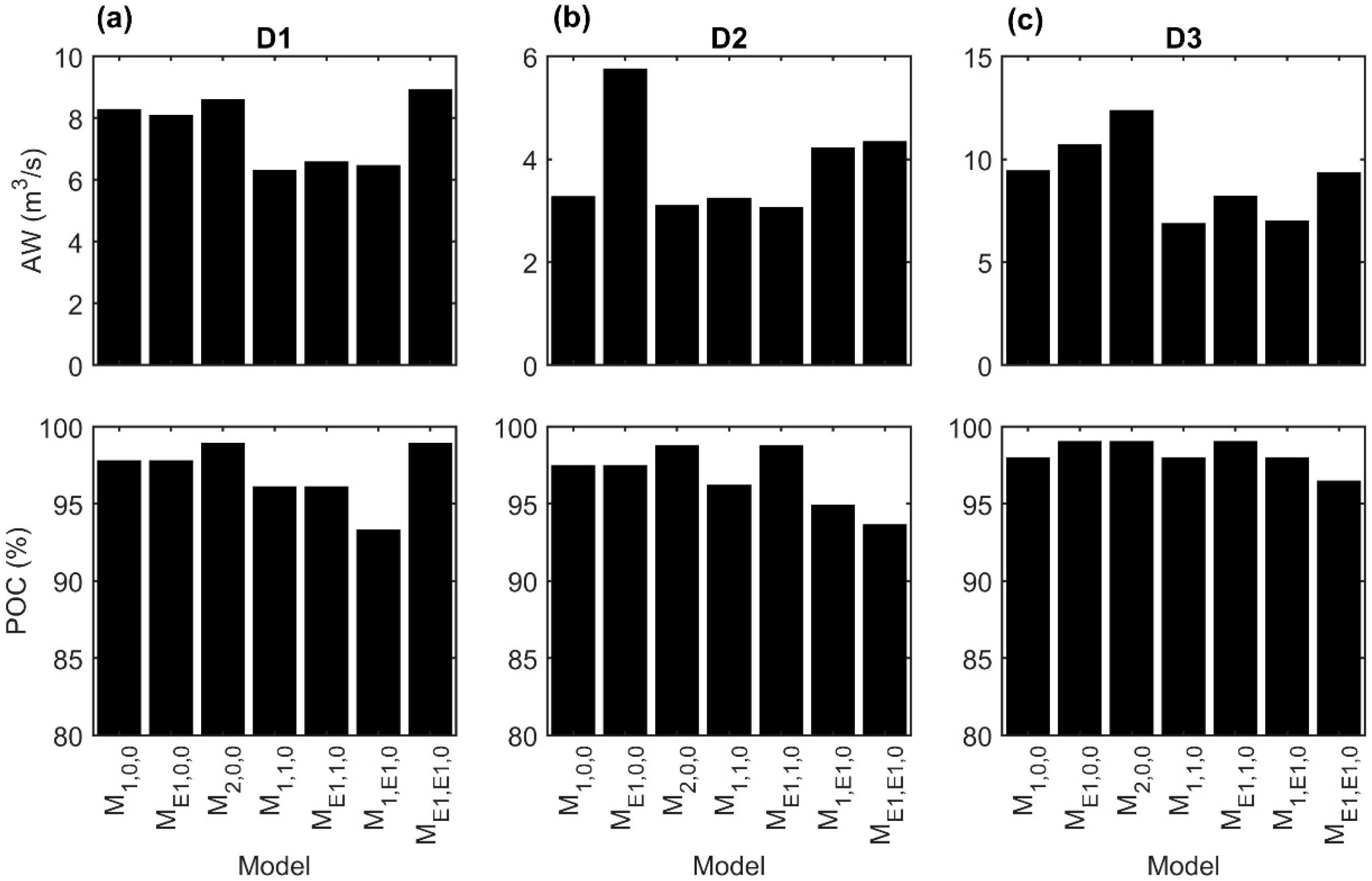
Moreover, Figure 2 displays the uncertainty metrics of all candidate nonstationary models for each dataset. For the D1, it appears that the optimal and top candidate models (${ℳ}_{1,0,0}$, ${ℳ}_{2,0,0}$, and ${ℳ}_{E1,0,0}$) selected in terms of the fitting efficiency (AIC and BIC) result in a relatively higher AW compared to other candidate models, while the high POCs (>95%) are reported in most of the models (except ${ℳ}_{1,E1,0}$) (Figure 2a). Recall that the AW and POC are two uncertainty metrics conflicting with each other, as a smaller AW can be achieved at the expense of decreasing the POC, and vice versa. In contrast, for the D2, the ${ℳ}_{E1,1,0}$ is not only optimal according to the fitting efficiency metrics but also superior in uncertainty, as it yields the lowest AW and the highest POC among the candidate models. Similarly, for the D3, the top models (${ℳ}_{1,1,0}$, ${ℳ}_{1,E1,0}$, and ${ℳ}_{E1,1,0}$) in general also offer a lower level of uncertainty than that of other competing models. Besides, the optimal model (${ℳ}_{1,1,0}$) selected in terms of fitting efficiency has the lowest AW and its POC is only 1% below the maximum POC reported in the ${ℳ}_{E1,0,0}$, ${ℳ}_{2,0,0}$, and ${ℳ}_{1,E1,0}$. Thus, the selected optimal models based on the fitting efficiency (AIC/BIC) do not always yield the lowest level of uncertainty (e.g., for the D1). These results argue that the optimal models selected in terms of the fitting efficiency might not necessarily guarantee to be optimal in terms of different assessment criteria, such as the uncertainty. Therefore, developing more elaborate criteria for incorporating the uncertainty into the selection of the optimal model might be beneficial for improving the NS-FFA, and, thus, the flood hazard assessment, as the reliability is also an important practical aspect of the analysis and assessment.

3.2. Flood Hazard Assessment under Nonstationarity

The selected optimal NS-FFA models, namely ${ℳ}_{1,0,0}$, ${ℳ}_{E1,1,0}$, and ${ℳ}_{1,1,0}$ for the D1, D2, and D3, respectively, are used to exemplify the temporal evolution of the flood hazard indexes. The nonstationarity in the three datasets is shown to be acceptably captured in the NS-FFA, as the nonstationary structures of the optimal models showcase coherence with the perceived patterns of nonstationarity of the underlying datasets as discussed previously. Among the three datasets, the D1 has the lowest degree of nonstationarity, as its estimated trend (Sen’s) slope in the mean is $0.02\tilde{\mu } {\mathrm{m}}^3/\mathrm{s}$ per decade (i.e., an upward trend with a slope of 2% per decade with respect to the reference statistic, in this case, the mean of the dataset). The degree of nonstationarity of the D3 is considered moderate among these datasets, as it shows a significant trend slope in the mean of $0.05\tilde{\mu } {\mathrm{m}}^3/\mathrm{s}$ per decade in the subperiod after the detected change point; whereas the slopes of the trends in the mean and standard deviation over the whole observation period (ignoring the change point) are $0.08\tilde{\mu } {\mathrm{m}}^3/\mathrm{s}$ per decade and $0.06\tilde{\sigma } {\mathrm{m}}^3/\mathrm{s}$ per decade, respectively. The D2 is considered to have the highest degree of nonstationarity among the datasets, as the slopes of its upward trends in the mean and standard deviation are $0.07\tilde{\mu } {\mathrm{m}}^3/\mathrm{s}$ per decade and $0.15\tilde{\sigma } {\mathrm{m}}^3/\mathrm{s}$ per decade, respectively.

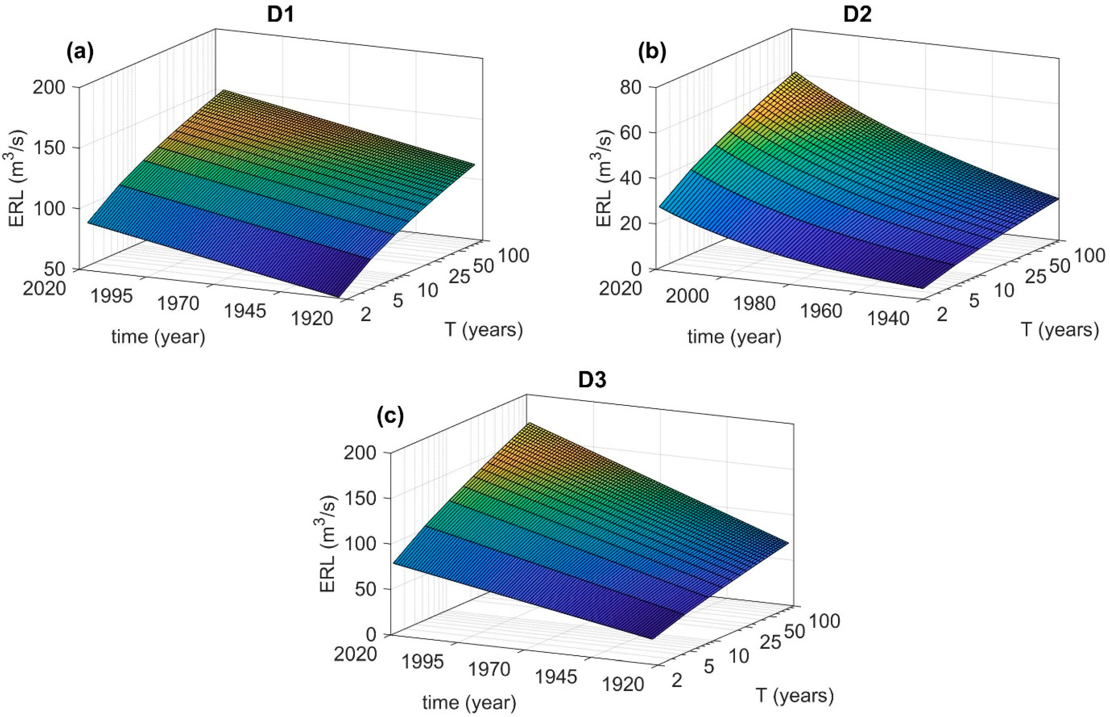
The frequency surfaces (Figure 3) present the temporal evolution of the point estimates of the ERLs. As expected, the ERLs increase with time at any given T for all three datasets. This behavior is consistent with the perceived upward trends in the mean and/or standard deviation in these datasets. Comparing the frequency surfaces of the datasets, the curvature of the frequency surface of the D2 is at a higher degree. Quantitatively, the ERLs increase at a constant rate of $0.03\widetilde{ERL} {\mathrm{m}}^3/\mathrm{s}$ per decade independently of the T and time for the D1. Here, $\widetilde{ERL}$ refers to the mean of the ERLs taken along the T-axis at every 5-yrs interval every year over the observation period. For the D3, the ERLs increase at an average rate of $0.09\widetilde{ERL} {\mathrm{m}}^3/\mathrm{s}$ per decade, while the trend slope varies along with the contour lines of Ts. For example, the ERLs increase at the rates of $0.07\widetilde{ERL} {\mathrm{m}}^3/\mathrm{s}$ and $0.10\widetilde{ERL} {\mathrm{m}}^3/\mathrm{s}$ per decade along with the contour lines of T = 5-yrs and 75-yrs, respectively. For the D2, the ERLs increase at the highest average rate of $0.16\widetilde{ERL} {\mathrm{m}}^3/\mathrm{s}$ per decade among the datasets, while the trend slopes of ERLs also vary with both the T and time. Thus, the variation pattern and degree of the ERLs appear to be consistent with the perceived pattern and degree of nonstationarity in the datasets.

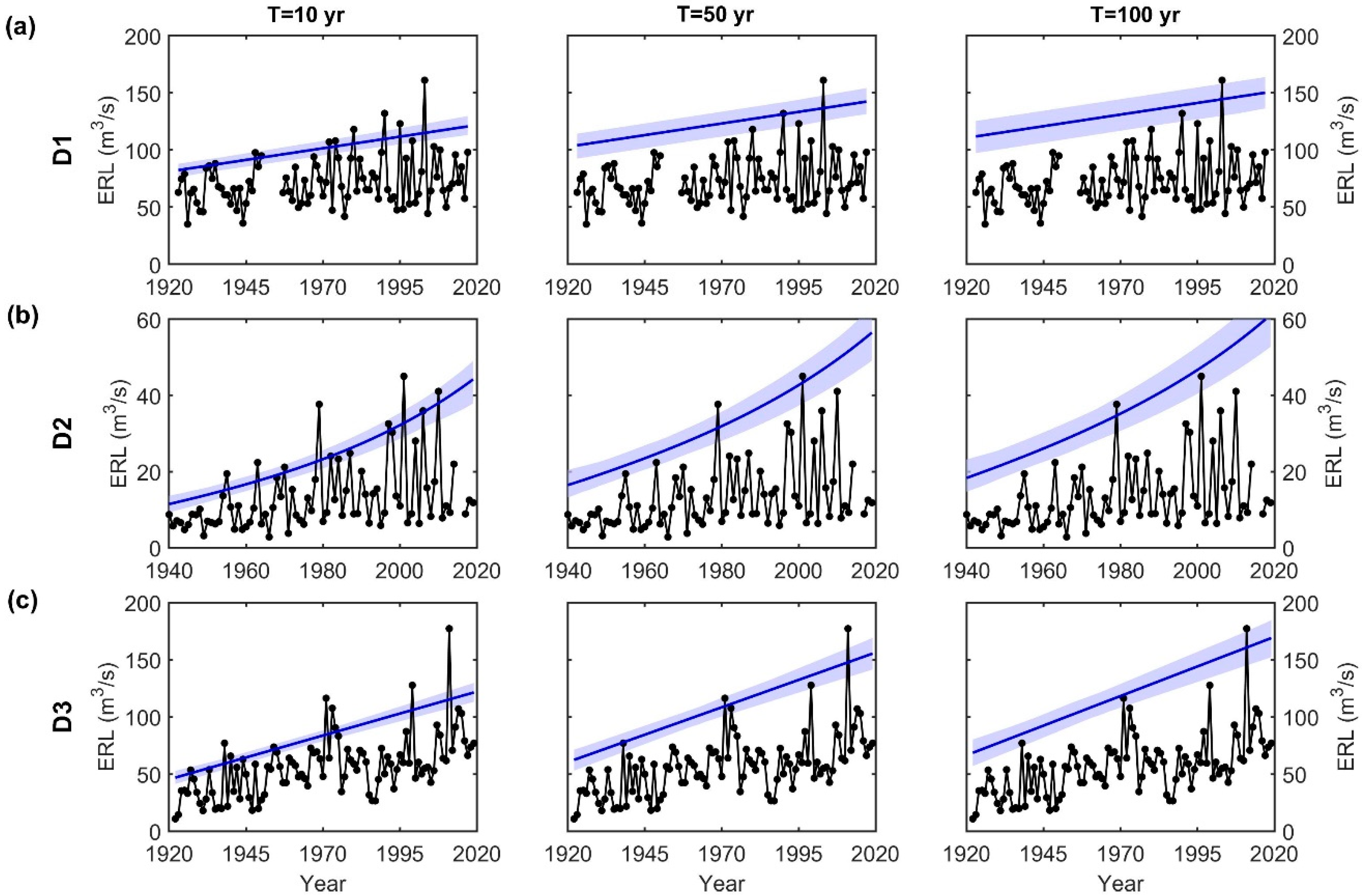
Figure 4 further depicts the point estimates of the ERLs corresponding to three selected Ts (10-, 50-, and 100-yr). As shown in Figure 4, the ERL point estimates of the three datasets tend to increase, indicating the rise of the expected quantiles associated with a given T. The most pronounced variations in the ERLs (and frequency surfaces) can be noticed in the D2, followed by the D3 and D1, which coincides with the most and least prominent degree of nonstationarity perceived in the D2 and D1, respectively. For instance, at the given T = 50-yr, the ERL point estimates for the D2 display an upward trend of $0.14{\overline{ERL}}_{50-yr} {\mathrm{m}}^3/\mathrm{s}$ per decade, whereas the trends are $0.09{\overline{ERL}}_{50-yr} {\mathrm{m}}^3/\mathrm{s}$ per decade and $0.03{\overline{ERL}}_{50-yr} {\mathrm{m}}^3/\mathrm{s}$ per decade for the D3 and D1, respectively. Note that significant upward trends were detected in both the mean and standard deviation in the D2 and D3 (over the entire observation period).

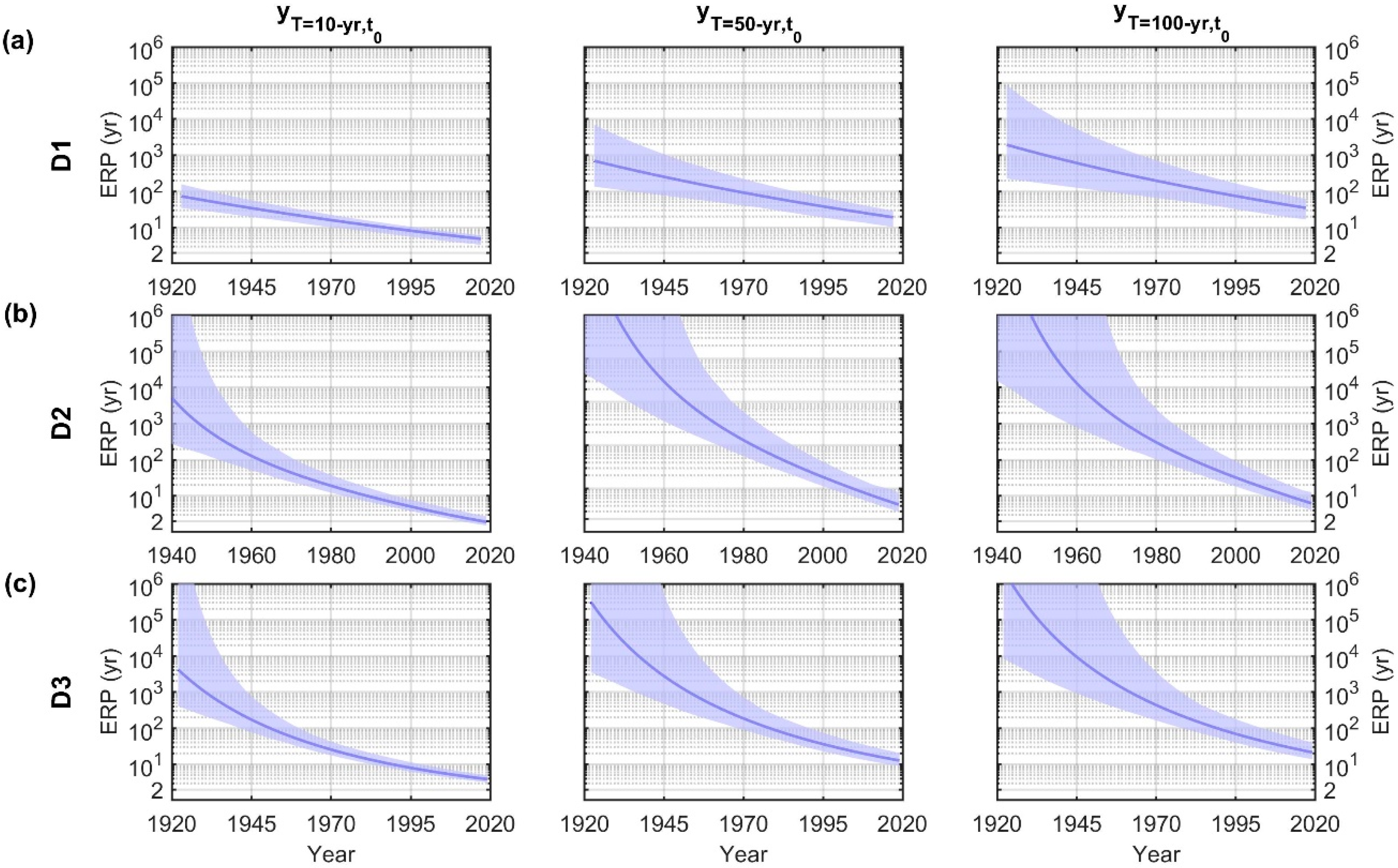
Figure 5 shows the point estimates of the ERPs corresponding to three assessment thresholds $y_{p_e,t_0}$ for D1, D2, and D3, respectively. These three $y_{p_e,t_0}$ are the 10-, 50- and 100-yr quantiles derived from the optimal nonstationary model at the reference time point ($t_0$). The selection of $t_0$ is problem specific. It can be the start time of the operation of the infrastructure under assessment or the start of the period of interest for policy evaluation. For illustration purposes, $t_0$ = 30 years prior to the end of the observation period of the datasets is used here. Differing from the point estimates of the ERL, the ERP point estimates tend to decrease temporally, suggesting the increase of the expected recurrence of $y_{p_e,t_0}$ over time for all three datasets. Furthermore, similar to the ERLs, a larger change in the ERP point estimates is resulted in when the degree of nonstationarity is higher. For example, at the given $y_{T=50-yr,t_0}$, the ERP point estimates for the D2 and D3 have (downward) average trends of $-656 yrs$ per decade and $-421 yrs$ per decade, respectively, whereas the trend for the D1 is $-42 yrs$ per decade. As illustrated in Figure 5, the extremely high point estimates of the ERP for the D2 and D3 (ERP > 10⁵ years for the reference assessment thresholds $y_{T=50yr,t_0}$ and $y_{T=100yr,t_0}$) might be unrealistic. Pertaining to the unrealistic estimates, Ouarda et al. [51] and Serinaldi and Kilsby [25] pointed out that the estimates of the flood quantiles and their exceedance probabilities can be sometimes unrealistic/improbable under nonstationarity. Thus, the estimates of the flood hazards might be unrealistic as well. A possible solution to avoid the unrealistic estimates might be to refine the nonstationary structure [25,51], such as through advancing the understanding of the cause–effect mechanism behind the nonstationarity.

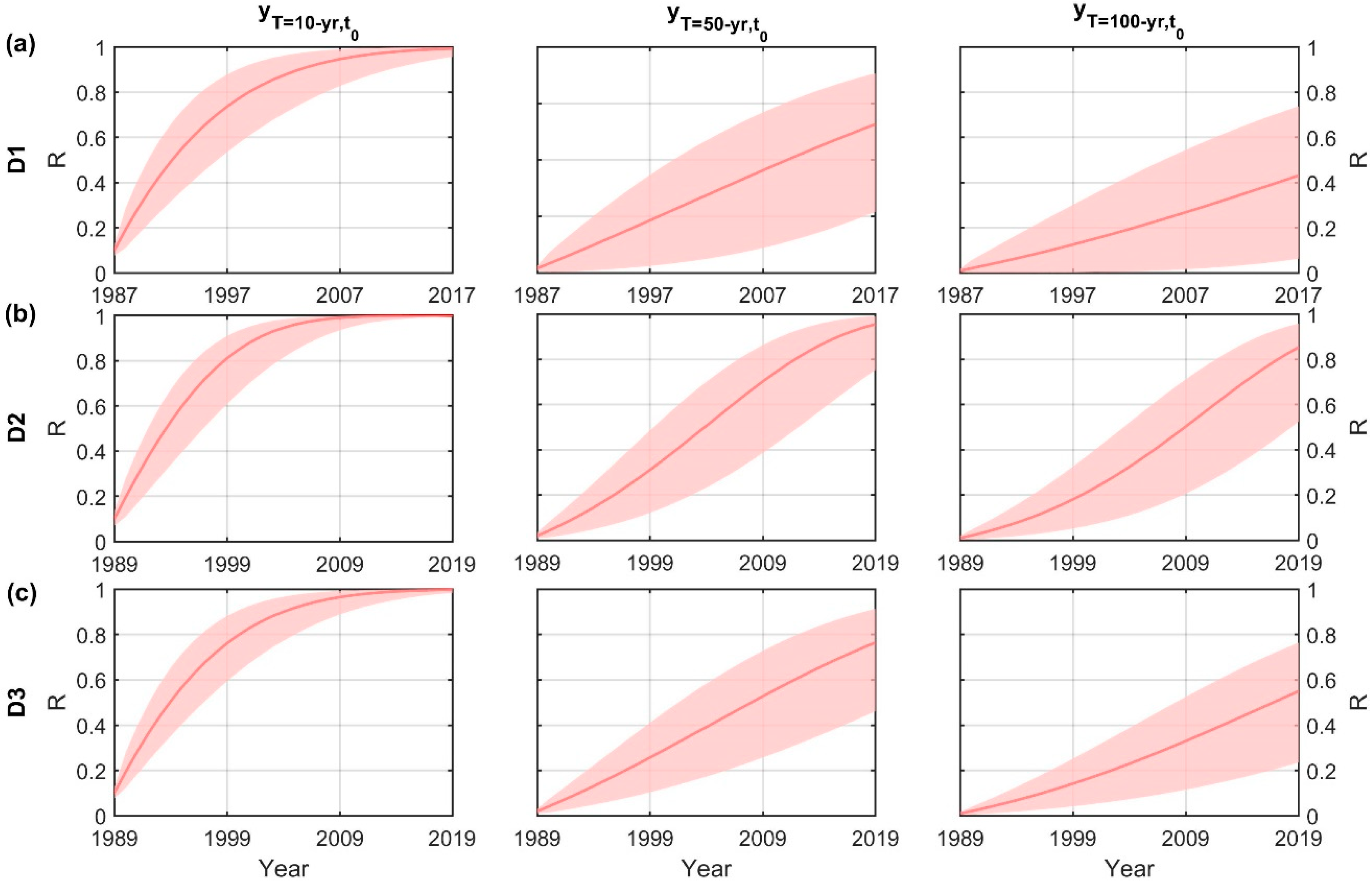
To exemplify the temporal evolution of the R, the $M$ is set to the last 30 years of the observation period. Thus, the $R$ is evaluated over the assessment horizon from the $t_0$ to the end of the observation period. The point estimates of the R at the previously defined three $y_{p_e,t_0}$ and their uncertainties are shown in Figure 6 for the three datasets. Comparing the R point estimates of these three datasets, the D2 always has the highest R (and the largest increase rate in R), while the lowest R is reported for the D1. For example, at the given $y_{T=50-yr,t_0}$, the R for the D1 increases at the average rate of $0.21$ per decade, whereas the R for the D3 and D2 increases at the rates of $0.26$ per decade and $0.35$ per decade, respectively. The results on the R along with the previous results on the ERL and ERP support that the flood hazards change more (increase or decrease) when the degree of nonstationarity of the underlying datasets is more pronounced. This implies that the impacts of climate change and other anthropogenic forces leading to the nonstationarity of flow AMSs on the flood hazards might be quantified according to the degree of nonstationarity. In addition, the trends in both the mean and standard deviation are shown to affect the flood hazards (e.g., in the D2 and D3). This calls for examining the temporal trends in the mean and standard deviation, and even higher order-moments if possible considering the sample size, to model and assess the effect of the nonstationarity on flood quantiles and hazards.

3.3. Uncertainty in the Flood Hazard Assessment

The application of the PF allows for the uncertainty estimation simultaneously with the point estimates of flood quantiles and hazards. As shown in Figure 4 and Figure 5, the uncertainty bandwidths of ERLs and ERPs, in general, increase with the increments of the T and $y_{p_e,t_0}$, respectively. These results illustrate that the hazard estimation is more uncertain in the tail region of the distribution compared to those events that are more recurrent. Moreover, the bandwidth of the ERL increases along with time at all three Ts for the three datasets. For instance, at the given T = 50-yr, the upward trend slopes of the ERL bandwidths are $0.01 AW$, $0.12 AW$, and $0.06 AW$ per decade for the D1, D2, and D3, respectively. Thus, the bandwidth of the ERL of the D2 increases at the highest rate among the datasets. Similar results were obtained at the given T = 10-yr and 100-yr. Therefore, the level of uncertainty in the ERL appears to elevate over time and its change rate is related to the degree of nonstationarity as well. This suggests that the elevation of the uncertainty in the ERLs would be more prominent when the degree of nonstationarity is higher. Similar to the trend in their point estimates, the bandwidth of the ERP decreases along with the time. It is worth it to mention that, at a certain time subperiod (i.e., the beginning of the evaluation period of the ERP), the uncertainties of the ERPs of the D2 and D3 are very large and range over a few orders of magnitude at the reference assessment thresholds of $y_{T=50yr,t_0}$ and $y_{T=100yr,t_0}$ (Figure 5).

As for the uncertainty in the R of the three datasets (Figure 6), the D1, which shows the lowest degree of nonstationarity, has the lowest R but the largest uncertainty; whereas the uncertainty in the R of the D2 is the lowest. For instance, at the given $y_{T=50-yr,t_0}$, the AW is 0.45, 0.34, and 0.35 for the D1, D2, and D3, respectively. Thus, different from its point estimates, the uncertainty in the R appears to be inversely correlated with the degree of nonstationarity of the datasets. From all the results of the ERL, ERP, and R, it can be concluded that despite the uncertainty in the flood hazard indexes respond differently to the nonstationarity, it is evidently associated with the nonstationary degree. The different responses of uncertainty in the flood hazard indexes to the nonstationarity would be ascribed to their different formulations, and, thus, their natures.

4. Conclusions

To advance the understanding of the impact of the nonstationarity on the flood hazards, this paper conducted the flood hazard assessment through the NS-FFA using the PF for three selected flow AMSs, which exhibit different nonstationary behavior and degree. In particular, the response of the flood hazards to the perceived pattern and degree of nonstationarity was investigated. In the NS-FFA, the nonstationary structure of the optimal models according to the fitting efficiency appeared to align with the perceived patterns of nonstationarity in these three underlying datasets, irrespective of their different patterns of nonstationarity. However, the optimal model selected in such a way did not always guarantee its superiority in terms of other assessment criteria, such as the uncertainty level in terms of the AW and/or POC, as illustrated in the D1. Therefore, to further improve the NS-FFA, and, thus, flood hazard assessment, it is desirable to incorporate the uncertainty into the selection of the optimal model, as the model reliability is the other important practical aspect of the frequency analysis. As for the flood hazard indexes, the responses of the three selected indexes, namely the ERL, ERP, and R (in both their point estimates and uncertainty levels) were also associated with the patterns and degrees of nonstationarity. Among the three datasets, the D2 having the most pronounced degree of nonstationarity was found to have the largest increases in the indexes; whereas the lowest increases in the indexes were calculated for the D1, which has the lowest degree of nonstationarity. Thus, the variations of the point estimates of the flood indexes intensified with the degree of nonstationarity, which should be characterized considering the temporal evolutions of the mean and standard deviation, and possibly the high-order moments. The uncertainties in the ERP and ERL tended to increase with the increase in the degree of nonstationarity. In contrast, the uncertainty in the R decreased with the increase in the degree of nonstationarity. As a result, the uncertainty in these flood hazard indexes showed different responses to the nonstationarity, depending on their formulations. All of these advocate the sensitivity of the flood hazards to the perceived patterns and degrees of nonstationarity of the underlying datasets. Therefore, the impacts of climate change and other anthropogenic factors on the flood hazards might be depicted by the nonstationarity characteristics of the datasets. On the other hand, further research on the effect of the PF on the NS-FFA, in particular in the context of the uncertainty in estimates, is recommended through comparing with other available approaches.

References

1. Tessler, Z.D.; Vorosmarty, C.J.; Grossberg, M.; Gladkova, I.; Aizenman, H.; Syvitski, J.P.M.; Foufoula-Georgiou, E. Profiling Risk and Sustainability in Coastal Deltas of the World. Science 2015, 349, 638–643. [Google Scholar] [CrossRef] [PubMed] [Green Version]
2. IPCC. Global Warming of 1.5 °C: Summary for Policymakers; World Meteorological Organization: Geneva, Switzerland, 2018. [Google Scholar]
3. Brooks, N.; Adger, W.N.; Kelly, P.M. The Determinants of Vulnerability and Adaptive Capacity at the National Level and the Implications for Adaptation. Glob. Environ. Chang. 2005, 15, 151–163. [Google Scholar] [CrossRef]
4. Milly, A.P.C.D.; Betancourt, J.; Falkenmark, M.; Hirsch, R.M.; Zbigniew, W.; Lettenmaier, D.P.; Stouffer, R.J.; Milly, P.C.D. Stationarity Is Dead: Whither Water Management? Science 2008, 319, 573–574. [Google Scholar] [CrossRef] [PubMed]
5. Faulkner, D.; Warren, S.; Spencer, P.; Sharkey, P. Can We Still Predict the Future from the Past? Implementing Non-Stationary Flood Frequency Analysis in the UK. J. Flood Risk Manag. 2020, 13, 1–15. [Google Scholar] [CrossRef] [Green Version]
6. Ray, L.K.; Goel, N.K. Flood Frequency Analysis of Narmada River Basin in India under Nonstationary Condition. J. Hydrol. Eng. 2019, 24, 1–15. [Google Scholar] [CrossRef]
7. Mondal, A.; Daniel, D. Return Levels under Nonstationarity: The Need to Update Infrastructure Design Strategies. J. Hydrol. Eng. 2019, 24, 1–11. [Google Scholar] [CrossRef]
8. Coles, S. An Introduction to Statistical Modeling of Extreme Values; Springer: London, UK, 2001. [Google Scholar]
9. Salas, J.D.; Obeysekera, J.; Vogel, R.M. Techniques for Assessing Water Infrastructure for Nonstationary Extreme Events: A Review. Hydrol. Sci. J. 2018, 63, 325–352. [Google Scholar] [CrossRef]
10. Cheng, L.; Aghakouchak, A. Nonstationary Precipitation Intensity-Duration-Frequency Curves for Infrastructure Design in a Changing Climate. Sci. Rep. 2014, 4, 1–6. [Google Scholar] [CrossRef] [Green Version]
11. Gado, T.A.; Van Nguyen, V.T. An At-Site Flood Estimation Method in the Context of Nonstationarity I. A Simulation Study. J. Hydrol. 2016, 535, 710–721. [Google Scholar] [CrossRef]
12. Villarini, G.; Smith, J.A. Flood Peak Distributions for the Eastern United States. Water Resour. Res. 2010, 46, 1–17. [Google Scholar] [CrossRef] [Green Version]
13. Sun, X.; Lall, U.; Merz, B.; Dung, N.V. Hierarchical Bayesian Clustering for Nonstationary Flood Frequency Analysis: Application to Trends of Annual Maximum Flow in Germany. Water Resour. Res. 2015, 51, 6586–6601. [Google Scholar] [CrossRef] [Green Version]
14. Mondal, A.; Mujumdar, P.P. Detection of Change in Flood Return Levels under Global Warming. J. Hydrol. Eng. 2016, 21, 1–12. [Google Scholar] [CrossRef]
15. Serago, J.M.; Vogel, R.M. Parsimonious Nonstationary Flood Frequency Analysis. Adv. Water Resour. 2018, 112, 1–16. [Google Scholar] [CrossRef]
16. Ouarda, T.B.M.J.; Yousef, L.A.; Charron, C. Non-Stationary Intensity-Duration-Frequency Curves Integrating Information Concerning Teleconnections and Climate Change. Int. J. Climatol. 2018, 2306–2323. [Google Scholar] [CrossRef] [Green Version]
17. Lu, F.; Song, X.; Xiao, W.; Zhu, K.; Xie, Z. Detecting the Impact of Climate and Reservoirs on Extreme Floods Using Nonstationary Frequency Models. Stoch. Environ. Res. Risk Assess. 2020, 34, 169–182. [Google Scholar] [CrossRef]
18. Dong, Q.; Zhang, X.; Lall, U.; Sang, Y.F.; Xie, P. An Improved Nonstationary Model for Flood Frequency Analysis and Its Implication for the Three Gorges Dam, China. Hydrol. Sci. J. 2019, 64, 845–855. [Google Scholar] [CrossRef]
19. Um, M.J.; Kim, Y.; Markus, M.; Wuebbles, D.J. Modeling Nonstationary Extreme Value Distributions with Nonlinear Functions: An Application Using Multiple Precipitation Projections for U.S. Cities. J. Hydrol. 2017, 552, 396–406. [Google Scholar] [CrossRef]
20. Olsen, J.R.; Lambert, J.H.; Haimes, Y.Y. Risk of Extreme Events under Nonstationary Conditions. Risk Anal. 1998, 18, 497–510. [Google Scholar] [CrossRef]
21. Wigley, T.M.L. The Effect of Changing Climate on the Frequency of Absolute Extreme Events. Clim. Chang. 2009, 97, 67–76. [Google Scholar] [CrossRef]
22. Parey, S.; Malek, F.; Laurent, C.; Dacunha-Castelle, D. Trends and Climate Evolution: Statistical Approach for Very High Temperatures in France. Clim. Chang. 2007, 81, 331–352. [Google Scholar] [CrossRef] [Green Version]
23. Parey, S.; Hoang, T.T.H.; Dacunha-Castelle, D. Different Ways to Compute Temperature Return Levels in the Climate Change Context. Environmetrics 2010, 21, 698–718. [Google Scholar] [CrossRef]
24. Katz, R.W.; Parlange, M.B.; Naveau, P. Statistics of Extremes in Hydrology. Adv. Water Resour. 2002, 25, 1287–1304. [Google Scholar] [CrossRef] [Green Version]
25. Serinaldi, F.; Kilsby, C.G. Stationarity Is Undead: Uncertainty Dominates the Distribution of Extremes. Adv. Water Resour. 2015, 77, 17–36. [Google Scholar] [CrossRef] [Green Version]
26. Read, L.K.; Vogel, R.M. Reliability, Return Periods, and Risk under Nonstationarity. Water Resour. Res. 2015, 6381–6398. [Google Scholar] [CrossRef]
27. Klemeš, V. Risk Analysis: The Unbearable Cleverness of Bluffing; Cambridge University Press: Cambridge, UK, 2002. [Google Scholar]
28. Aven, T.; Pörn, K. Expressing and Interpreting the Results of Quantitative Risk Analyses. Review and Discussion. Reliab. Eng. Syst. Saf. 1998, 61, 3–10. [Google Scholar] [CrossRef]
29. Borgomeo, E.; Mortazavi-Naeini, M.; Hall, J.W.; Guillod, B.P. Risk, Robustness and Water Resources Planning Under Uncertainty. Earth’s Futur. 2018, 6, 468–487. [Google Scholar] [CrossRef] [Green Version]
30. Obeysekera, J.; Salas, J.D. Quantifying the Uncertainty of Design Floods under Nonstationary Conditions. J. Hydrol. Eng. 2014, 19, 1438–1446. [Google Scholar] [CrossRef]
31. Renard, B.; Sun, X.; Lang, M. Bayesian Methods for Non-Stationary Extreme Value Analysis. In Extremes in a Changing Climate; Springer: Berlin/Heidelberg, Germany, 2013; pp. 39–95. [Google Scholar]
32. Sen, S.; He, J.; Kasiviswanathan, K.S. Uncertainty Quantification Using the Particle Filter for Non-Stationary Hydrological Frequency Analysis. J. Hydrol. 2020, 584. [Google Scholar] [CrossRef]
33. Vidrio-Sahagún, C.T.; He, J.; Kasiviswanathan, K.S.; Sen, S. Stationary Hydrological Frequency Analysis Coupled with Uncertainty Assessment under Nonstationary Scenarios. J. Hydrol. 2020, 125725. [Google Scholar] [CrossRef]
34. Salamon, P.; Feyen, L. Assessing Parameter, Precipitation, and Predictive Uncertainty in a Distributed Hydrological Model Using Sequential Data Assimilation with the Particle Filter. J. Hydrol. 2009, 376, 428–442. [Google Scholar] [CrossRef]
35. Moradkhani, H.; Hsu, K.-L.; Gupta, H.; Sorooshian, S. Uncertainty Assessment of Hydrologic Model States and Parameters: Sequential Data Assimilation Using the Particle Filter. Water Resour. Res. 2005, 41, 1–17. [Google Scholar] [CrossRef] [Green Version]
36. Shrestha, D.L.; Solomatine, D.P. Machine Learning Approaches for Estimation of Prediction Interval for the Model Output. Neural Netw. 2006, 19, 225–235. [Google Scholar] [CrossRef] [PubMed]
37. Alvisi, S.; Franchini, M. Fuzzy Neural Networks for Water Level and Discharge Forecasting with Uncertainty. Environ. Model. Softw. 2011, 26, 523–537. [Google Scholar] [CrossRef]
38. Doucet, A.; de Freitas, N.; Gordon, N. An Introduction to Sequential Monte Carlo Methods; Springer: New York, NY, USA, 2001. [Google Scholar] [CrossRef]
39. Gordon, N.J.; Salmond, D.J.; Smith, A.F.M. Novel Approach to Nonlinear/Non-Gaussian Bayesian State Estimation. IEE Proc. F Radar Signal Process. 1993, 140, 107. [Google Scholar] [CrossRef] [Green Version]
40. Milly, P.C.D.; Betancourt, J.; Falkenmark, M.; Hirsch, R.M.; Kundzewicz, Z.W.; Lettenmaier, D.P.; Stouffer, R.J.; Dettinger, M.D.; Krysanova, V. On Critiques of “Stationarity Is Dead: Whither Water Management?”. Water Resour. Res. 2015. [Google Scholar] [CrossRef] [Green Version]
41. Bayazit, M. Nonstationarity of Hydrological Records and Recent Trends in Trend Analysis: A State-of-the-Art Review. Environ. Process. 2015, 2, 527–542. [Google Scholar] [CrossRef]
42. Matalas, N.C. Comment on the Announced Death of Stationarity. J. Water Resour. Plan. Manag. 2012, 138, 311–312. [Google Scholar] [CrossRef]
43. Lindgren, G.; Rootzén, H.; Sandsten, M. Stationary Stochastic Processes for Scientists and Engineers; Chapman and Hall/CRC: Boca Raton, FL, USA, 2013. [Google Scholar]
44. Liu, J.; Zhang, Q.; Singh, V.P.; Gu, X.; Shi, P. Nonstationarity and Clustering of Flood Characteristics and Relations with the Climate Indices in the Poyang Lake Basin, China. Hydrol. Sci. J. 2017, 62, 1809–1824. [Google Scholar] [CrossRef]
45. Yan, L.; Xiong, L.; Liu, D.; Hu, T.; Xu, C.Y. Frequency Analysis of Nonstationary Annual Maximum Flood Series Using the Time-Varying Two-Component Mixture Distributions. Hydrol. Process. 2017, 31, 69–89. [Google Scholar] [CrossRef]
46. Gado, T.A.; Nguyen, V.T. Van. An At-Site Flood Estimation Method in the Context of Nonstationarity II. Statistical Analysis of Floods in Quebec. J. Hydrol. 2016, 535, 722–736. [Google Scholar] [CrossRef]
47. Byun, K.; Hamlet, A.F. A Risk-Based Analytical Framework for Quantifying Non-Stationary Flood Risks and Establishing Infrastructure Design Standards in a Changing Environment. J. Hydrol. 2020, 584, 124575. [Google Scholar] [CrossRef]
48. Vu, T.M.; Mishra, A.K. Nonstationary Frequency Analysis of the Recent Extreme Precipitation Events in the United States. J. Hydrol. 2019, 575, 999–1010. [Google Scholar] [CrossRef]
49. Yan, L.; Li, L.; Yan, P.; He, H.; Li, J.; Lu, D. Nonstationary Flood Hazard Analysis in Response to Climate Change and Population Growth. Water 2019, 11, 1811. [Google Scholar] [CrossRef] [Green Version]
50. El Adlouni, S.; Ouarda, T.B.M.J.; Zhang, X.; Roy, R.; Bobée, B. Generalized Maximum Likelihood Estimators for the Nonstationary Generalized Extreme Value Model. Water Resour. Res. 2007, 43, 1–13. [Google Scholar] [CrossRef]
51. Ouarda, T.B.M.J.; Charron, C.; St-Hilaire, A. Uncertainty of Stationary and Nonstationary Models for Rainfall Frequency Analysis. Int. J. Climatol. 2019, 1–20. [Google Scholar] [CrossRef]
52. Arulampalam, M.S.; Maskell, S.; Gordon, N.; Clapp, T. A Tutorial on Particle Filters for Online Nonlinear/Non-Gaussian Bayesian Tracking. IEEE Trans. Signal Process. 2002, 50, 174–188. [Google Scholar] [CrossRef] [Green Version]
53. Sarhadi, A.; Soltani, S.; Modarres, R. Probabilistic Flood Inundation Mapping of Ungauged Rivers: Linking GIS Techniques and Frequency Analysis. J. Hydrol. 2012, 458–459, 68–86. [Google Scholar] [CrossRef]
54. Sun, P.; Wen, Q.; Zhang, Q.; Singh, V.P.; Sun, Y.; Li, J. Nonstationarity-Based Evaluation of Flood Frequency and Flood Risk in the Huai River Basin, China. J. Hydrol. 2018, 567, 393–404. [Google Scholar] [CrossRef]
55. Hsu, K.-L.; Gupta, H.V.; Sorooshian, S. Artificial Neural Network Modeling of the Rainfall-Runoff Process. Water Resour. Res. 1995, 31, 2517–2530. [Google Scholar] [CrossRef]
56. Akaike, H. A New Look at the Statistical Model Identification. IEEE Trans. Automat. Contr. 1974, 19, 716–723. [Google Scholar] [CrossRef]
57. Hosking, J.R.M. L-Moments: Analysis and Estimation of Distributions Using Linear Combinations of Order Statistics. J. R. Stat. Soc. 1990, 52, 105–124. [Google Scholar] [CrossRef]
58. Xiong, L.; Wan, M.; Wei, X.; O’connor, K.M. Indices for Assessing the Prediction Bounds of Hydrological Models and Application by Generalised Likelihood Uncertainty Estimation/Indices Pour Évaluer Les Bornes de Prévision de Modèles Hydrologiques et Mise En Œuvre Pour Une Estimation d’incertitude. Hydrol. Sci. J. 2009, 54, 852–871. [Google Scholar] [CrossRef] [Green Version]
Figure 1. Selected three datasets, (a) D1, (b) D2, and (c) D3, and their perceived patterns of nonstationarity. The solid and dashed lines indicate the significant trends in the mean and the standard deviation, respectively.
Geosciences 11 00013 g001
Figure 2. Uncertainty metrics (average bandwidth (AW) and percentage of coverage (POC) of the candidate nonstationary models for the datasets, (a) D1, (b) D2, and (c) D3.
Geosciences 11 00013 g002
Figure 3. Frequency surfaces for the three datasets, (a) D1, (b) D2, and (c) D3.
Geosciences 11 00013 g003
Figure 4. The point estimates of the effective return levels (ERLs) (blue lines) and their uncertainty (shaded areas) at the three given return periods (T) (10-, 50-, and 100-yr) for the three datasets, (a) D1, (b) D2, and (c) D3 (c).
Geosciences 11 00013 g004
Figure 5. The point estimates of the effective return periods (ERPs) (blue lines) and their uncertainty (shaded areas) at the three selected assessment thresholds ( y p e , t 0 ) (the 10-, 50-, and 100-yr quantiles derived from the corresponding nonstationary model at the reference time t 0 = 30 years prior to the end of the observation period) for (a) D1, (b) D2, and (c) D3.
Geosciences 11 00013 g005
Figure 6. The point estimates of the risk of failure (R) (red lines) and their uncertainty estimates (shaded areas) at the three selected assessment thresholds ( y p e s ) (the 10-, 50-, and 100-yr quantiles derived from the corresponding nonstationary model at the reference time t 0 = 30 years prior to the end of the observational period) for the three datasets, (a) D1, (b) D2, and (c) D3.
Geosciences 11 00013 g006