Burial-Deformation History of Folded Rocks Unraveled by Fracture Analysis, Stylolite Paleopiezometry and Vein Cement Geochemistry: A Case Study in the Cingoli Anticline (Umbria-Marche, Northern Apennines)

Abstract

Unravelling the burial-deformation history of sedimentary rocks is prerequisite information to understand the regional tectonic, sedimentary, thermal, and fluid-flow evolution of foreland basins. We use a combination of microstructural analysis, stylolites paleopiezometry, and paleofluid geochemistry to reconstruct the burial-deformation history of the Meso-Cenozoic carbonate sequence of the Cingoli Anticline (Northern Apennines, central Italy). Four major sets of mesostructures were linked to the regional deformation sequence: (i) pre-folding foreland flexure/forebulge; (ii) fold-scale layer-parallel shortening under a N045 σ₁; (iii) syn-folding curvature of which the variable trend between the north and the south of the anticline is consistent with the arcuate shape of the anticline; (iv) the late stage of fold tightening. The maximum depth experienced by the strata prior to contraction, up to 1850 m, was quantified by sedimentary stylolite paleopiezometry and projected on the reconstructed burial curve to assess the timing of the contraction. As isotope geochemistry points towards fluid precipitation at thermal equilibrium, the carbonate clumped isotope thermometry (Δ₄₇) considered for each fracture set yields the absolute timing of the development and exhumation of the Cingoli Anticline: layer-parallel shortening occurred from ~6.3 to 5.8 Ma, followed by fold growth that lasted from ~5.8 to 3.9 Ma.

1. Introduction

The reconstruction of the burial-deformation history of sedimentary rocks is a complex issue but an essential exercise to understand the tectonic and sedimentary history in fold-and-thrust belts and foreland basins, with numerous implications spanning from the evolution of the fluid-flow system and associated resources to the understanding of the long-term behavior of the upper crust [1,2,3,4,5,6,7]. Mesostructures observed in fold-and-thrust belts and related forelands, such as faults, veins, and stylolites provide essential information for understanding the deformation pattern [8]. Numerous studies have indeed linked the development of fractures to the large-scale long-term folding history and geometry, either through a descriptive field-based approach [9,10,11], paleostrain and paleostress reconstructions [12,13,14,15,16,17], mechanical simulation (e.g., [18,19]), or through geochemical approaches (e.g., [20]). Besides, studies of distributed subseismic fractures demonstrated that mesostructures are markers of the local deformation sequences and provide access to the evolution of the associated paleostresses [8,9,10,15,21,22,23,24,25,26,27,28,29,30,31,32,33,34,35,36]. When it comes to the burial history, however, the depth-time paths are reconstructed from temperature-dependent proxies, such as organic matter thermal maturity, temperature-dependent clay minerals (e.g., [37,38,39]), fluid inclusion microthermometry, or low temperature thermochronology (apatite fission tracks, U-Th/He on apatite crystals [40,41,42,43,44,45,46]). All these methods rely on the occurrence of specific features (organic matter, fluid inclusions, specific minerals like zircons, or Ar-rich clays) and return only partial information (e.g., maximum temperature, timing of reaching closure temperature…) while requiring assumptions about the past geothermal gradient. The latter is often argued over in fold-and-thrust belts and foreland basins where uplift and erosion are common events, thus it remains strongly challenging to reconstruct the burial at which the deformation occurred [7].

We propose to build on recent methodological advances to better constrain the timing of deformation in fold-and-thrust belts and foreland basins. The development of U-Pb dating on calcite cement enables absolute dating on the tectonic vein filling and synkinematic clay minerals (e.g., [47,48,49]), clumped isotopes can be reliably used to reconstruct the exact temperature of precipitation under 90–100 °C [50], and its combination to fluid inclusion microthermometry allows to reconstruct the temperature-pressure-time path in sedimentary sequence [51]. Moreover, the understanding of how stylolites can be used as stress gauges [52,53] enables reconstruction of the burial experienced by sedimentary rocks (e.g., [7,54,55,56,57,58,59,60]). These methods rely on the ubiquitous features of carbonate rocks, and we propose in this contribution to combine paleopiezometry and isotope-based thermometry as a new methodology widely applicable to carbonates in order to assess the timing and depth of burial/contraction during deformation history. We present an original application by reconstructing the burial-deformation history of the carbonate sedimentary sequence of the Cingoli Anticline, an arcuate fold in the Umbria-Marche Apennines Ridge (UMAR, Northern Apennines, central Italy; Figure 1). The Cingoli Anticline is an excellent case study for testing such new methodologies: (i) it is a rather simple symmetrical fold, mainly formed by carbonate rocks exhibiting pervasive fractures and stylolites [61]; (ii) there is an abundant literature that discusses the timing of folding, based on sedimentologic and tectonic studies [62,63,64]; (iii) the geothermal gradient is known [65]; and (iv) it belongs to a young mountain belt where the past mesostructures received relatively poor attention [60,61,66,67,68,69,70] compared to their active counterparts.

In this study, we aim at identifying, characterizing and dating the mesostructures related to the main stages of deformation, i.e., faults, fractures, and stylolites linked to layer-parallel shortening (LPS), folding, and late-stage fold tightening (LSFT). For this purpose, we first carry out a classical field-based mesotructural study. We further reconstruct the burial history of strata by building burial curves using present strata thickness corrected for physical and chemical compaction and by applying the roughness inversion technique to sedimentary stylolites in order to quantify the maximal vertical stress, and hence the maximum burial depth experienced by the sedimentary sequence prior to contraction and during exhumation.

The timing of the deformation is further constrained by the temperatures derived from isotopic data (¹⁸O,¹³C and clumped isotopes), showing a thermal equilibrium with the host rocks considering previously published geothermal gradients, and compared to previous studies carried out in nearby folds [60,71]. This original and transferable approach reveals the burial evolution, the timing of deformation, and the fluid system in the Cingoli Anticline during the Apennine contraction in eastern UMAR.

2. Geological Setting

2.1. The Umbria Marche Apennine Ridge (UMAR)

The Apennines fold-and-thrust belt extends from the Po Plain to the Calabrian Arc over a distance of 1500 km, and it is the result of the Eurasian and African Plates convergence [72,73]. The Apennine belt accommodated significant orogenic contraction, estimated up to 50% through cross section balancing [74], and recorded shortening rates ranging from 6 mm/year up to 15-50 mm/year [74,75]. From a structural point of view, the Apennine belt is characterized by a succession of asymmetrical anticlines with eastward vergence, separated by narrower and often asymmetrical synclines. The Apennines are commonly divided into two main arcs, the Northern and the Southern Apennines arcs, each associated with its own geological and structural characteristics [76,77,78]. Moreover, this curved belt, with eastward convexity, is increasingly younger from west to east (from Oligocene to Pleistocene; [72,79]). This is the result of a roughly eastward migration of the deformation front (and its associated successive foredeep basin), which is related to the eastward retreating subduction of the Adriatic Plate under the European Plate, superimposed by post-orogenic extension at the rear of the propagating orogenic belt [29,72,80,81].

The UMAR represents the central-southern part of the Northern Apennines arc developed during late Miocene-Pliocene when the area was involved in the Apennines build-up. It is about 450 km long and rises to over 2000 m above sea level [75]. The sedimentary succession observed in the UMAR can be divided into three main units as follows: (i) Upper Triassic evaporites, the thickness of which is estimated at 1000 m before deformations and considered as a décollement level. They unconformably overlie crystalline rocks of the basement, which is barely or not even observable at the outcrop [72]; (ii) the Umbria-Marche carbonate-dominated succession (~2500 m thick), divided in several formations deposited from the earliest Jurassic to Oligocene [72,82,83,84]; (iii) Miocene hemipelagites and turbidites, deposited above these carbonate rocks, which record the progressive eastward involvement of the Meso-Cenozoic succession into the fold-and-thrust belt [62,85]. Indeed, during the foredeep stage, more than 3000 m of turbidites were deposited ahead of the advancing fold-and-thrust belt.

Both thick- and thin-skinned structural styles of deformation have been proposed for the Apennines. The thin-skinned interpretation considers a disharmonic deformation of the crust with the sedimentary units detached along the Triassic evaporites [86,87,88]. The thin-skinned model is opposed to the thick-skinned which considers the involvement of the basement during compressional deformation (e.g., [89]) Furthermore, several studies suggest that many thrusts are rooted on inherited pre-orogenic structures, mostly pre-existing normal faults formed either during the evolution of the Mesozoic passive margin or during the foreland flexure [90,91,92,93,94,95,96].

The UMAR undergoes the following main stages of regional deformation: (i) the forebulge stage consisting of the foreland flexuring [8], dated from late Oligocene-early Miocene in the western part of the ridge (i.e., eastern Tuscany-Monte Nero) and from middle Miocene in the eastern part of the ridge (i.e., Gubbio, San Vicino, and Cingoli areas) [79]; (ii) the LPS event, a pre/early-folding compressional stage NE-SW-oriented related to the Apenninic contraction [66,97,98,99], occurred by early Miocene to the west, and by middle Pliocene to the east [79]; (iii) the folding stage, started by early Miocene in the western part of the UMAR, and by middle Miocene in the eastern part. This stage is characterized by a maximum stress trending parallel to regional shortening, i.e., NE-SW-oriented [29], and local extension perpendicular to fold axis and associated with strata curvature at fold hinge [60]; (iv) the LSFT, associated with a NE-SW contractional trend. This stage corresponds to the moment when shortening is no longer accommodated, by e.g., limb rotation [60]; (v) a post-orogenic extension, starting by Miocene times in the western UMAR [99] and by early Pliocene times in the eastern part of the ridge [62,63], and continuing today. This extensional stage is associated with NNW-SSE trending related normal faults causing the downfaulting of the fold succession [86,99,100].

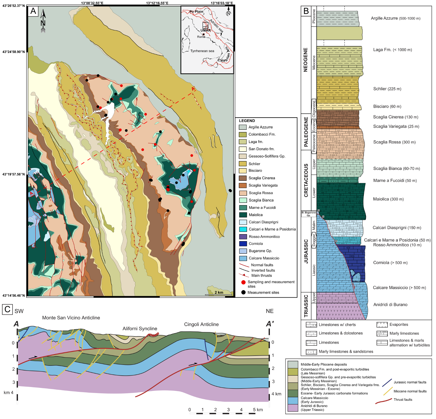
2.2. The Cingoli Anticline

2.2.1. Structural Pattern

The Cingoli Anticline is located in the eastern part of the UMAR along the footwall of the Sibillini Mountains (Figure 1A). This anticline is characterized by an arcuate geometry; its main NW-SE axis evolves toward a N-S orientation in its southern part; it is characterized by gently dipping limbs and its hinge is relatively flat. The fold has a spatial extension of about 15 km from north to south, and about 5 km from west to east and it culminates ~400 m above the local land (770 m above sea level). An WNW-ESE oriented left-lateral fault and a NNE-SSW oriented right-lateral fault bound the Cingoli Anticline to the north and south, respectively (Figure 1A). In addition, [101] and [63] suggest that inherited pre-contractional structures striking ~N-S (i.e., the Jurassic rifting and the late Miocene foreland flexure) strongly controlled the subsequent contractional tectonic evolution of the area (Figure 1A,C).

2.2.2. Sedimentary Succession

Where not specified, the lithostratigraphic units described below are traditional and validated units [102], and correspond with formation-rank units.

The deformed units comprise Mesozoic and Cenozoic marine deposits, consisting of evaporites and platform carbonates at the base overlain by pelagic carbonates [63,64,101,103] (Figure 1B). The succession comprises:

(1)

Upper Triassic anhydrites and dolostones, grouped in the Anidridi di Burano, unconformably deposited above the continental deposits of the Verrucano and the Hercynian basement; at the top of the Anidridi di Burano, euxinic interstratified marls are present.

(2)

The Calcare Massiccio, formed by massive peridital limestones dated from Hettangian to Sinemurian (ca. 201–191 Ma).

(3)

Four main Jurassic formations: (i) the Corniola, limestones with cherts beds (early Sinemurian–early Toarcian, ca. 199–183 Ma); (ii) the Rosso Ammonitico, nodular marly limestones dated Toarcian (ca. 183–174 Ma); (iii) the marls and cherty limestones of the Calcari e Marne a Posidonia (late Toarcian-early Bajocian, ca. 174–170 Ma); (iv) the Calcari Diasprigni, dominated by radiolarian-rich cherty limestones and cherts and, on top, by micritic limestones and marls bearing abundant Saccocoma sp. fragments (late Bajocian-early Tithonian, ca. 170–152 Ma). Because of the horst and graben structures related to the Jurassic extensional tectonics, these deposits accumulated in the hanging wall basins forming thick (hundreds of meters) “basinal” successions, while thin (up to few tens of meters), fossil-rich and condensed successions (Bugarone Group) accumulated on top of footwall blocks of Jurassic faults during the same time span (i.e., from early Pliensbachian to early Tithonian; ca. 191–152 Ma) [82,83,104,105,106].

(4)

The Maiolica, micritic limestones associated with chert beds (Tithonian–earliest Aptian, ca. 152–124 Ma).

(5)

Shales and marls of the Marne a Fucoidi (Aptian-Albian, ca. 124–100 Ma).

(6)

The “Scaglia” group is composed of micritic limestones with cherts intercalations (late Aptian-Aquitanian, ca. 113–21 Ma), and divided into four formations: (i) the Scaglia Bianca (Cenomanian-earliest Turonian, ca. 100–94 Ma); (ii) the Scaglia Rossa (earliest Turonian-Lutetian, ca. 94–41 Ma), subdivided into three members; (iii) the Scaglia Variegata (Lutetian-Priabonian, ca. 48–34 Ma) and (iv) the Scaglia Cinerea (Rupelian-earliest Aquitanian, ca. 34–22 Ma).

(7)

Bisciaro (Aquitanian-Burdigalian, ca. 22–16 Ma) and Schlier (Langhian-Tortonian, ca. 16–7 Ma) formations, hemipelagic limestones, marly limestones and marls.

(8)

Siliciclastic foredeep deposits, grouped in two major sequences: (i) Messinian arenitic and pelitic turbidites (ca. 7–5 Ma), composed by the Laga formation and the Gessoso-Solfifera Group with the San Donato and Colombacci formations; (ii) arenites, pelites and fossiliferous marine clays and marls of the Argille Azzure, early to middle Pliocene in age (ca. 5–3 Ma). In this area, the Messinian and Pliocene deposits are continuous and widespread, and provide an almost complete record of the deformation history of the ridge’s outer domains. In particular, growth strata observed in the San Donato and Colombacci formations within the Aliforni Syncline postdate flexural turbidites of the Laga formation, consequently broadly constraining fold growth to late Messinian-Zanclean (ca. 6–4 Ma) [62,63].

3. Materials and Methods

3.1. Fracture-Stylolite Network Characterization and Striated Fault Planes Analysis

The structural data collection and sampling sites are distributed along the whole anticline (Figure 1). The characterization of the fracture-stylolite network is based on field observations and measurements and analyses of joints, veins, striated faults, and tectonic stylolites. The dataset comprises more than 2300 orientations of mesostructures from the Cingoli Anticline. Furthermore, abutment and crosscutting relationships were carefully observed and analysed to establish the relative chronology of fracture sets. Fracture orientation data were projected on Schmidt stereodiagrams (lower hemisphere), in the current attitude of the strata (raw) and after unfolding (unfolded). In addition, the major sets of joints and/or veins (i.e., the most documented and representative at fold scale) were grouped and averaged by a Fisher statistical analysis, based on the following assumptions: (i) similar orientation considering natural variability (i.e., within 20°); (ii) deformation mode (e.g., opening, shearing, contraction), defined through thin sections observed with optical microscope; and (iii) chronological relationships.

Considering that stylolite peaks grow parallel to the main shortening direction [107], with respect to the distribution of dissolution gradients (i.e., non-soluble particles) [108], the orientation of the horizontal maximum principal stress (σ₁) was inferred from the maximum density of the peak orientation of tectonic stylolites. The early, syn-, and late folding sets of mesostructures were discriminated with the OpenStereo software [109]. Data were corrected for bedding attitude, by rotation about a horizontal axis to remove the dip angle of the strata, in order to investigate the relationships between fracturing and folding. Thus, fractures were grouped according to their geographical and structural position (respectively north/south and forelimb/backlimb), and according to the main stages of deformation.

Approximately 40 mesoscale striated faults were also measured to complement this mesostructural analysis, in 3 sites of measurements located in the northern and southern ends of the anticline. We used Angelier’s inversion technique [110] which, under specific assumptions [111], allowed us to calculate paleostress orientations (i.e., local trend and plunge of principal stress axes) and stress ratios for each site of measurement.

3.2. Rock Mechanical Properties

To calculate the mechanical properties of the studied rocks, we used the Schmidt rebound hammer technique, which is a non-destructive method used for the estimation of the uniaxial compressive strength and Young modulus of concrete and natural rocks (e.g., [112]). It implies the use of a spring-loaded piston (the Schmidt hammer), pressed orthogonally against a surface of rock. The energy created by the resistance of the surface to the impact enables the piston to rebound. The distance traveled by the piston after the rebound is called the rebound value R, which is considered to be a proxy of the surface hardness [112], itself used to quantify uniaxial compressive strength and Young modulus of the rock [113]. A Silver Schmidt OS8200 (manufactured by PROCEQ) was used on 12 sites in various localities and sedimentary units of the fold. Each site consists of 50 to 90 rebounds performed perpendicularly to the surface, in most case lying flat (i.e., the hammer being vertical), from which rebound values were averaged as a single rebound value valid for the site. In order to ensure that this value is free from any outlier due to local heterogeneity, we calculated a moving average incremental mean until the mean rebound value stabilizes (supplementary material, Figure S1, Table S1).

3.3. Sedimentary Stylolite Roughness Inversion

Sedimentary stylolites are pressure-solution surfaces usually developed parallel to bedding in sub-horizontal strata during burial, i.e., when σ₁ was vertical. They are frequently observed in sedimentary rocks, and especially in carbonates. The 1D roughness of a track along these dissolution surfaces, i.e., the difference in height between two points along the track (sensu [53]), results from a competition between two forces [53]: (i) roughening forces, i.e., pinning on non-soluble particles in the rocks, and (ii) smoothing forces, associated with the surface energy at scale <1 mm and the elastic energy at scale >1 mm. Two main scaling regimes are discriminated by the stylolite growth model [56,107,108,114] depending on the predominant energy and the associated Hurst exponent (i.e., roughness exponent): the surface energy-controlled scale, characterized by a steep-slope and a roughness exponent of 1.1 ± 0.1, and the elastic energy-controlled scale, associated with a gentle slope and a Hurst exponent between 0.5 and 0.6. At the transition of these scale regimes, the change in roughness exponent is associated with a crossover length, estimated in mm by the signal processing approach. The authors in [53] directly link this crossover length L_c to the magnitude of prevalent mean stress σ_m and differential stress σ_d in the strata at the time the stylolite stopped to be an active dissolution surface, with Equation (1):

$${\mathrm{L}}_{\mathrm{c}}=\frac{\mathsf{\gamma }\mathrm{E}}{{\mathsf{\beta }\mathsf{\sigma }}_{\mathrm{m}}{\mathsf{\sigma }}_{\mathrm{d}}}$$

(1)

where L_c is the crossover length converted to m, E the Young modulus of the rock (in Pa), γ is the solid-fluid interfacial energy (in J·m⁻²), and β a dimensionless constant depending on the Poisson ratio (ν) and calculated with the relation:

$$\mathsf{\beta }=\frac{\mathsf{\nu }(1-2\mathsf{\nu })}{\mathsf{\pi }}$$

(2)

The mean stress and the differential stress, are defined in Pa according to the Equations (3) and (4):

$${\mathsf{\sigma }}_{\mathrm{m}}=\frac{{\mathsf{\sigma }}_1{+\mathsf{\sigma }}_2{+\mathsf{\sigma }}_3}{3}$$

(3)

$${\mathsf{\sigma }}_{\mathrm{d}}{=\mathsf{\sigma }}_1{-\mathsf{\sigma }}_3$$

(4)

Several studies successfully applied this approach, establishing the spectral analysis of the roughness of sedimentary stylolites as a robust paleopiezometry tool [54,57,59,60,108,115,116,117,118], especially because the final roughness is acquired quickly at the end of the stylolite’s growth, thus depends only on stress and no longer on strain rate [108].

More than 100 sedimentary stylolites, with peaks perpendicular to the dissolution plane, were sampled in several localities of the Cingoli Anticline (Figure 1A) in the Maiolica, Scaglia Rossa, and Scaglia Variegata. The samples were cut and polished to better analyze the stylolite track. Each cut was made perpendicular to the plane of the stylolite and scanned with a resolution of 12,800 pixels per inches; the resulting file is an image on which the 1D track was hand drawn at magnifications 200% and 400% for greater precision. Then, each track was analyzed as a periodic signal. Usual analyses involve the Fourier Power Spectrum (FPS) and Average Wavelet Coefficient (AWC) methods [115]. We chose the method of Average Wavelet spectrum with Daubechies D4 wavelets [115,119], which is proven to be more stable and less sensitive to resolution effects. We used a non-linear regression with fixed Hurst coefficients of 0.5 and 1.1, corresponding to elastic and surface regimes, respectively (please refer to supplementary material, Figure S2, for the plots). The uncertainty for this regression approach to estimate L_c has been previously estimated to 23% [57]. To calculate the vertical stress magnitude, the horizontal stress was then considered as isotropic (i.e., uniaxial strain hypothesis, σ_v> σ_h = σ_H) in the case of sedimentary stylolites. Thus, the Equation (1) established by [53] is simplified as:

$${\mathsf{\sigma }}_{\mathrm{v}}{}^2=\frac{\mathsf{\gamma }\mathrm{E}}{{\mathsf{\alpha }\mathrm{L}}_{\mathrm{c}}}$$

(5)

α being a constant defined as follows:

$$\mathsf{\alpha }=\frac{\left(1-2\mathsf{\nu }\right){(1+\mathsf{\nu })}^2}{{30\mathsf{\pi }(1-\mathsf{\nu })}^2}$$

(6)

To verify this assumption, sections perpendicular to the stylolite plane were cut for several samples and treated following the same inversion method, the isotropy of the horizontal stress implying a constant value of the crossover length regardless of the track direction [53,115].

While the solid-fluid interfacial energy γ is well-known and stable, fixed to 0.24 J·m⁻² for dolomite and of 0.32 J·m⁻² for calcite [120], and while the Poisson ratio ν is rather stable in carbonates and can be approximated to 0.25 ± 0.05, a major source of uncertainty lies in the values of the Young modulus E [57,121]. With known E, ν, and γ, the uncertainty on the calculated stress is 12% [57]. As in previous works [57,60,117,118] the calculated vertical stress ${\mathsf{\sigma }}_{\mathrm{v}}=$ σ₁ was translated directly into the burial depth (z) of rocks using the relation

$${\mathsf{\sigma }}_{\mathrm{v}}=\varrho \mathrm{gz}$$

(7)

with ϱ the average dry density of overlying rocks and g the gravity acceleration. Indeed, the stylolite roughness can be considered as unaffected by local fluid overpressure because the dissolution is located along a fluidic film [56,108,116], an assumption that remains valid until the system is fluidized [122]. For this reasons, ρ was considered as the average dry rock density for clastic and carbonate sediments (evaluated mean value at 2400 kg·m⁻³), without any additional assumption on the past thermal gradient or fluid pressure [7], and g the gravity acceleration, fixed at 9.8 m·s⁻².

3.4. O-C Stable Isotopes

The analysis of stable oxygen and carbon isotopes, associated with the study of the diagenetic state of the rocks, allows for the identification and characterization of fluid generations at the origin of mineralization and vein filling within sedimentary rocks [20,123,124,125,126,127,128,129]. We focus hereinafter on the calcite cements filling the tectonic veins related either to LPS or to strata curvature at fold hinges. The mineralogy of some host-rock was checked with X-ray diffraction (supplementary material, Figure S3) using a Bruker D2 Phaser diffractometer from the ISTeP laboratory (Sorbonne Université) with X-Ray wavelength of 1.54056 Å. The resulting X-ray patterns showing mostly pure calcite with minor amounts of quartz. The diagenetic state of calcite veins was checked under cathodoluminescence microscopy and were performed on a cold cathode Cathodyne platform (CITL CCL 8200 Mk4) at stable vacuum of 60 mThor, a voltage of 12 kV, and a current of 200 µA, corresponding to the ideal voltage-current conditions to activate the luminescence of the carbonates.

We selected vein cements where the vein texture [130] and the diagenetic state support a single phase of filling, occurring at the same time or soon after fracture development (e.g., elongated blocky, Figure 2).

The isotope ratios of oxygen (¹⁸O/¹⁶O) and carbon (¹³C/¹²C) of samples collected in several localities of the Cingoli Anticline were obtained by Isotope-Ratio Mass Spectrometry (IRMS). The spectrometric equipment couples an automatic sample preparation line (KIEL IV) and an analysis section (DELTA V advantage) from Thermo Fisher Scientific at the ISTeP laboratory (Paris). We first selected veins of which (i) the cement witnessed a single growth step, unaltered by later diagenetic events, checked with cathodoluminescence microscopy; and (ii) the cement was likely related to vein opening, considering antitaxial or elongated blocky textures [130]. Thirty (30) to 50 μg of powder were sampled from the vein and the surrounding host-rocks as well, using a computer assisted micromill drill. The powder was reacted with anhydrous orthophosphoric acid at 70 °C to extract CO₂ gas, itself ionized in the spectrometer. The measured isotopic ratio reported in permil relative to the Vienna Pee Dee Belemnite (‰VPDB) are with an accuracy of 0.05‰ and 0.1‰ for carbon and oxygen, respectively.

3.5. Carbonate Clumped-Isotope Paleothermometry (Δ₄₇)

All analyses were performed at the Laboratoire des Sciences du Climat et de l’Environnement (LSCE, Gif sur Yvette). Eight samples of homogenized carbonate powder were converted to CO₂ by anhydrous phosphoric acid reaction at 90 °C in a common, stirred acid bath for 15 minutes. Initial phosphoric acid concentration was 103% (1.91 g/cm³) and each batch of acid was used for 7 days. After the cryogenic removal of the water, the evolved CO₂ was helium-flushed at 25 mL/mn through a purification column packed with Porapak Q (50/80 mesh, 1 m length, 2.1 mm ID) and held at −20 °C, and then quantitatively recollected by cryogenic trapping and transferred into an Isoprime 100 dual-inlet mass spectrometer equipped with six Faraday collectors (m/z 44–49). Each analysis took about 2.5 hours, during which the analyte gas and working reference gas were allowed to flow from matching, 10 mL reservoirs into the Nier-type ion source through deactivated fused silica capillaries (65 cm length, 110 μm ID). Every 20 minutes, gas pressures were adjusted to achieve m/z = 44 current of 80 nA, with differences between analyte gas and working gas generally below 0.1 nA. Pressure-dependent background current corrections were measured 12 times for each analysis. All background measurements from a given analytical session are then used to determine a mass-specific relationship linking background intensity (Zm), total m/z = 44 intensity (I44), and time (t):

Zm = a + bI44 + ct + dt²

(8)

Background-corrected ion current ratios (δ⁴⁵ to δ⁴⁹) were converted to δ¹³C, δ¹⁸O, and “raw” Δ₄₇ values as described by [131], using the IUPAC oxygen-17 correction parameters. The isotopic composition (δ¹³C, δ¹⁸O) of our working reference gas was computed based on the nominal isotopic composition of carbonate standard ETH–3 [132] and an oxygen-18 acid fractionation factor of 1.00813 [133]. Raw Δ₄₇ values were then converted to the “absolute” Δ₄₇ reference frame defined by the “ETH” carbonate standards [132] using regression methods detailed by [134]. Full analytical errors are derived from the external reproducibility of unknowns and standards (N_f = 78) and conservatively account for the uncertainties in raw Δ₄₇ measurements as well as those associated with the conversion to the “absolute” Δ₄₇ reference frame. The precipitation temperature was calculated using the calibration proposed by [135] and updated by [132].

3.6. Burial Model

The burial model associated with the Cingoli Anticline area was constructed from the open access well data collection of the ViDEPI project selected around the Cingoli Anticline (i.e., Misa1, Rosora1, Burano1, Treia1 wells). Thicknesses were sequentially uncompacted to obtain burial depths of the strata of interest through time. Two kinds of corrections were therefore applied, considering the effects of both physical and chemical compaction. The computer interface used to produce these burial curves is the Backstrip software, which performs 1D backstripping of sedimentary strata [136] and involves several parameters for modeling.

First, the layer thicknesses were corrected for chemical compaction, in order to be referenced in the software. Thickness information was provided by stratigraphic studies or well data (i.e., current formation thicknesses). In this case, thicknesses were corrected for chemical compaction, considering spacing and amplitudes of bedding-parallel stylolites (BPS) for each formation studied. The average number of sedimentary stylolites per meter was estimated from outcrop data. The height of the highest tooth (i.e., the height from tooth to base line) associated with each analyzed stylolite was also computed from the samples. Chemical compaction was then deduced from these two parameters, calculated as their product, and expressed as a percentage of bed thickness.

The second step consisted of defining parameters needed to evaluate physical compaction undergone by the different layers, related to the weight of the sedimentary column and possibly of the water column (according to the type of basin considered). These parameters, such as the dry density ρ and the porosity coefficient c, were defined on the basis of the work by [137,138], as follows: (i) the dry density ρ was chosen at 2700 kg/m³ for carbonate rocks and 1800 kg/m³ for other lithologies; (ii) the porosity coefficient c was calculated with the following equations and the porosity-depth curves established by [137,138]. Φ is the porosity at depth y, while Φ₀ the surface porosity, both given by the curves.

$${\mathsf{\Phi }=\mathsf{\Phi }}_0{\mathrm{e}}^{-\mathrm{cy}}\mathrm{with}\mathrm{c}=\frac{1}{\mathrm{y}}\ln \left(\frac{\mathsf{\Phi }}{{\mathsf{\Phi }}_0}\right)$$

(9)

Thus, c is equal to 0.58 for carbonate rocks and to 0.3 for other lithologies. Corrections related to the weight of sediments and water being significantly different [137,138], the type of basin was also defined (0 for a marine basin, 1 for a continental basin), in order not to introduce bias into the resulting burial curves.

4. Results

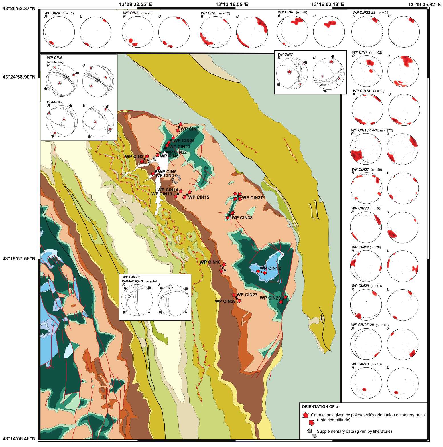
4.1. Fracture-Stylolite Network Characterization and Striated Fault Planes Analysis

The fracture deformation mode was defined through thin sections observed with optical microscope, either by considering the texture (i.e., elongate blocky or crack-seal), or the object shift in the matrix (Figure 2).

Three major sets of fractures were discriminated on the basis of their average orientation (Figure 3 and Figure 4A,B) whereas their chronological sequence was established through abutment and crosscutting relationships at different scales (from outcrop to thin section):

-

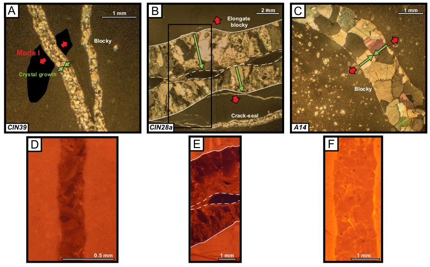
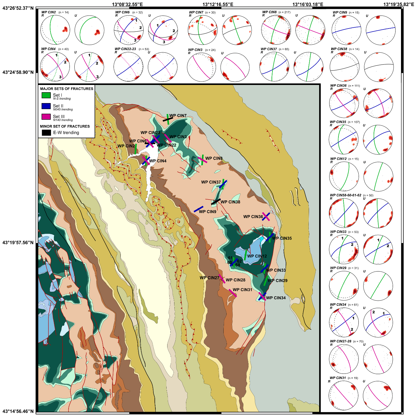
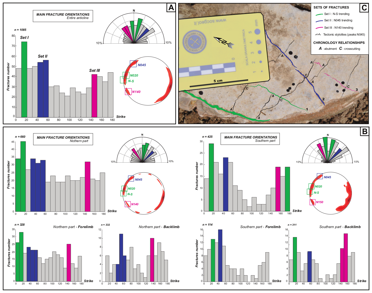
set I gathers bedding-perpendicular joints oriented N180 to N020 (after unfolding). This set is observed over the entire anticline, predates sets II and III, because it is intersected and abutted by a set of stylolites with peaks oriented N045, which are themselves intersected and abutted by the joints/veins of set II (Figure 4C).

-

set II gathers joints and veins with N045 ± 10° orientation, present throughout the study area. They are perpendicular to bedding strike. This set postdates set I and predates set III.

-

set III comprises bedding-perpendicular N130 to N160-oriented joints parallel to bedding strike (i.e., N135-140 in the North and N160 in the South). They are mainly parallel to the axis of the anticline and crosscut or abut all other joint/vein sets (Figure 4C).

-

another set of E-W fractures, poorly represented at the scale of the anticline (i.e., only in the northern part, in three sites of measurements), includes N070 to N110-oriented joints (after unfolding) and perpendicular to the bedding, developed after set II. Because of the low number of measurements (i.e., 25 of 3000 fractures analyzed) and because they systematically developed near faults (Figure 3), this family of fractures is considered as minor and of local meaning only, and therefore not affiliated to a major set. Consequently, it will not be interpreted thereafter.

Tectonic stylolite peaks are mostly oriented N045 (Figure 5). The continuous change in dip of the stylolite plane from vertical to oblique suggests that part of the tectonic stylolites developed before folding and other after folding. Few prefolding stylolites peaks are oriented N140 (WP CIN 37 and WP CIN 27–28) in the Maiolica and Scaglia in the southern backlimb, and N090 in Calcare Massiccio in the southern part of the anticline (WP CIN 12).

The inversion of striated faults for stress was carried out in few sites in the anticline (Figure 5):

-

in the northern backlimb, conjugate NW-SE trending reverse faults reveal a compressional stress regime with a σ₁ axis roughly oriented N045;

-

in the northern forelimb, N170–180-oriented normal faults indicate either an extensional regime with σ₃ oriented N045, or, more likely correspond to tilted oblique-slip reverse faults consistent with a pre-tilting N020 compression;

-

in the southern backlimb, the few fault-slip data preclude any reliable stress tensor calculation. The dataset is however consistent with a post-tilting σ₁ oriented N045 and σ₃ oriented N135.

4.2. Young Modulus Estimate

Rock elastic properties were measured on flat homogeneous surfaces, for Maiolica, Scaglia Rossa and Scaglia Variegata, corresponding to 12 sites of measurement (n = 1063). For each site, the mean for rebound value R was represented as a function of the number of rebound incorporated in the mean calculation (supplementary material, Figure S1, Table S1); the stabilized R value (represented as a plateau on the graph) is then believed to be corrected from heterogenous effect and outliers, and so represent the rebound value R for the rock studied. Strikingly, the average of these representative R values is similar in the Maiolica, Scaglia Rossa and Scaglia Variegata formations, with values of 45 ± 8.4, 48 ± 5.8 and 46 ± 8.5, respectively. R values were further interpreted as Young moduli following the empiric relationship determined in [113] for sedimentary rocks and return a E value similar for the 3 formations at about 20 GPa, very similar to the one reconstructed from stylolite inversion by [121] of 23 GPa.

4.3. Sedimentary Stylolite Roughness Inversion

The stylolite roughness inversion method was applied on 112 BPS sampled in the northern, central and southern parts of the Cingoli Anticline (Figure 1A), within the Cretaceous to Eocene carbonate formations. The inversion was successful (i.e., returning a value of crossover length L_c) on 77 BPS covering the anticline and distributed as follows: Maiolica (early Cretaceous, n = 56), Scaglia Rossa (late Cretaceous-early Eocene, n = 18) and Scaglia Variegata (middle to late Eocene, n = 3). For several stylolites, this paleopiezometric inversion was applied on two orthogonal tracks, in order to ensure that the stress on the horizontal plane was isotropic. L_c values are summarized in

Table 1. Results of stylolite roughness inversion, applied on bedding-parallel stylolites.

Sample	GPS	Formation	Lc (mm)	σv (MPa) *	Depth (m)
CIN13	58	Maiolica	0.44 ± 0.10	34	1440
			0.60 ± 0.14	29	1250
			0.77 ± 0.18	26	1100
			0.84 ± 0.19	24	1040
			0.30 ± 0.07	41	1740
			0.27 ± 0.06	43	1840
			0.31 ± 0.07	40	1700
CIN14	59	Maiolica	0.34 ± 0.08	38	1630
			0.63 ± 0.14	28	1200
CIN3	60	Maiolica	0.39 ± 0.09	36	1540
			0.54 ± 0.12	30	1300
			0.49 ± 0.11	32	1360
CIN6	60	Maiolica	0.54 ± 0.12	30	1300
			0.36 ± 0.08	37	1550
CIN8	60	Maiolica	0.53 ± 0.12	30	1300
			0.76 ± 0.17	26	1100
CIN9	60	Maiolica	0.39 ± 0.09	36	1540
CIN10	60	Maiolica	0.36 ± 0.08	37	1600
			0.31 ± 0.07	40	1700
			0.29 ± 0.07	42	1800
CIN15	61	Maiolica	0.49 ± 0.11	32	1360
			0.84± 0.19	25	1040
			0.38 ± 0.09	37	1550
CIN17	61	Maiolica	0.85 ± 0.20	25	1040
CIN18	61	Maiolica	0.45 ± 0.10	33	1400
			0.91 ± 0.21	23	1000
			1.09 ± 0.25	22	900
CIN33	64	Maiolica	0.73 ± 0.17	26	1100
			1.08 ± 0.25	22	900
			0.46 ± 0.11	33	1400
			0.34 ± 0.08	38	1630
CIN38	64	Maiolica	0.53 ± 0.12	30	1300
			0.55 ± 0.13	30	1300
CIN40	64	Maiolica	0.76 ± 0.17	26	1100
			0.46 ± 0.11	33	1400
			0.32 ± 0.07	40	1700
			0.56 ± 0.13	30	1300
			0.35 ± 0.08	38	1600
C3	WP_CIN3	Maiolica	1.76 ± 0.40	17	720
			1.38 ± 0.32	19	810
C51	WP_CIN23	Maiolica	1.18 ± 0.27	21	880
			0.67 ± 0.15	27	1150
C56	WP_CIN23	Maiolica	0.35 ± 0.08	38	1600
C67′	WP_CIN29	Maiolica	0.75 ± 0.17	26	1100
			0.58 ± 0.13	29	1250
C68	WP_CIN29	Maiolica	0.33 ± 0.08	39	1650
C69	WP_CIN29	Maiolica	0.74 ± 0.17	26	1100
			0.46 ± 0.11	33	1400
C70	WP_CIN29	Maiolica	0.35 ± 0.08	38	1600
			0.34 ± 0.08	38	1600
C71	WP_CIN29	Maiolica	0.38 ± 0.09	36	1540
C72	WP_CIN29	Maiolica	0.50 ± 0.12	32	1350
C86	WP_CIN38	Maiolica	1.33 ± 0.31	20	850
			0.39 ± 0.09	36	1540
			0.43 ± 0.10	34	1450
			1.11 ± 0.26	22	900
C79	WP_CIN36	Scaglia Rossa	0.38 ± 0.09	37	1550
C15	WP_CIN7	Scaglia Rossa	0.49 ± 0.11	32	1300
			0.51 ± 0.12	32	1300
C87	WP_CIN8	Scaglia Rossa	1.17 ± 0.27	21	880
			0.75 ± 0.17	26	1100
C21	WP_CIN9	Scaglia Rossa	0.59 ± 0.14	29	1250
			0.68 ± 0.16	27	1150
			0.45 ± 0.10	34	1420
C26	WP_CIN13	Scaglia Rossa	0.87 ± 0.20	24	1020
			0.85 ± 0.20	24	1020
			0.98 ± 0.23	23	960
C28	WP_CIN13	Scaglia Rossa	0.45 ± 0.10	33	1400
C29	WP_CIN13	Scaglia Rossa	0.63 ± 0.14	28	1200
			0.64 ± 0.15	28	1200
			0.84 ± 0.19	25	1040
C30	WP_CIN14	Scaglia Rossa	0.36 ± 0.08	38	1600
			0.60 ± 0.14	29	1230
			0.40 ± 0.09	35	1500
C2	WP_CIN2	Scaglia Variegata	0.75 ± 0.17	26	1100
			1.26 ± 0.29	20	850
			1.75 ± 0.40	17	720

∗ Crossover length given within 23% uncertainty. Vertical stress σ_v given within 12% uncertainty calculated according to Equation (5), considering a Young modulus E = 23 GPa ([139], this study), a Poisson ratio ν = 0.25, and interfacial energy γ = 0.32 J·m⁻². Depth calculated using dry density of rock d = 2400 g·m⁻³, acceleration of gravity g = 9.81 m·s⁻².

, and reported as an interval for each formation studied, considering an uncertainty of 23%:

-

Maiolica: [0.27 ± 0.06; 1.76 ± 0.40] mm

-

Scaglia Rossa: [0.36 ± 0.08; 1.17 ± 0.27] mm

-

Scaglia Variegata: [0.75 ± 0.17; 1.75 ± 0.40] mm

4.4. Burial Model

The burial curves resulting from the backstripping process are presented in Figure 6.

They were reconstructed for the Triassic to Pliocene formations in the Cingoli area, considering: (i) the chemical compaction calculated at 8% for Maiolica, and 3% for Scaglia Rossa and Scaglia Variegata considering spacing and amplitude of BPS (following [108]); (ii) physical compaction by using the open-source software BackStrip [136]. The temperatures linked to these depths were calculated by considering a geothermal gradient of 23 °C·km-1 reconstructed in the outermost western part of the UMAR from organic matter thermal maturity [65] and clay minerals [140] (Figure 6). These curves illustrate a first phase of increasing burial, corresponding to the deepening of the Umbria-Marche basin and a second phase of exhumation since early Pliocene. The maximum burial depths computed for the formations of interest, and equivalent temperatures, can be deduced from the left and right y-axis of Figure 6, respectively. These curves are consistent with models established for the inner part of the belt in the area of the Monte Tancia thrust [71].

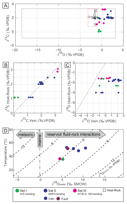
4.5. Oxygen and Carbon Stable Isotopes

Twenty-eight (28) vein calcite cements and surrounding calcite host-rocks from the Scaglia Rossa were analyzed for δ₁₈O and δ₁₃C (

Table 2. Results of Stable Isotopic Analyses of Oxygen and Carbon Isotopes.

		Vein		Host-Rock
Sample	Set	δ13C (‰VPDB)	δ18O (‰VPDB) Calcite	δ13C (‰VPDB)	δ18O (‰VPDB) Calcite
CIN23-V1	I	2.04	2.19	2.15	−2.95
CIN23-V2	I	1.90	−0.44	2.15	−2.95
CIN23-V3	I	1.91	−1.56	2.15	−2.95
CIN23-V4	I	1.98	−0.68	2.15	−2.95
CIN25-V1	I	2.06	1.79	2.10	−2.27
CIN25-V2	I	2.06	−0.97	2.10	−2.27
CIN25-V3	I	2.08	2.07	2.10	−2.27
CIN39-V1	I	0.05	−0.74	1.08	−1.59
CIN39-V2	I	0.10	−0.30	1.08	−1.59
CIN39-V3	I	0.31	−0.66	1.08	−1.59
CIN7-V1	II	2.48	1.37	2.47	−1.68
CIN7-V2	II	2.97	2.09	2.47	−1.68
CIN28a-V1	II	2.07	1.21	2.01	−1.82
CIN28a-V2	II	1.81	0.58	2.01	−1.82
CIN28a-V3	II	1.95	2.22	2.01	−1.82
CIN26-V1	II	2.00	2.59	2.02	−1.74
CIN26-V2	II	1.95	2.34	2.02	−1.74
CIN26-V3	II	2.14	1.47	2.02	−1.74
CIN26-V4	II	2.05	1.38	2.02	−1.74
CIN28b-V1	II	2.08	2.20	2.03	−1.64
CIN28b-V2	II	1.98	1.68	2.03	−1.64
A13-V1	III	3.23	0.79	3.08	−1.45
A14-V1	III	3.21	0.21	2.89	−1.53
A14-V2	III	3.19	0.61	2.89	−1.53
CIN37-V1	III	1.39	−0.59	1.09	−1.55
CIN37-V2	III	1.25	0.46	1.09	−1.55
CIN37-V3	III	1.10	−1.12	1.09	−1.55
CIN37-V3	III	1.10	−1.12	1.09	−1.55

, Figure 7).

In the host-rock (n = 11), the δ¹⁸O isotopic values range from −2.95 to −1.45‰VPDB while the δ¹³C isotopic values range from 1.08 to 3.08‰VPDB. In the calcite veins (n = 28), the δ¹⁸O isotopic values range from −1.56 to 2.59‰VPDB while the δ¹³C isotopic values range from 0.05 to 3.23‰VPDB. The vein cements show variable isotopic values: for the set I (N-S, n = 10), δ¹⁸O ratio ranges from −1.56 to 2.19‰VPDB while δ¹³C ratio ranges from 0.05 to 2.08‰VPDB; for the set II (N045, n = 11), δ¹⁸O ratio ranges from 0.58 to 2.59 ‰VPDB while δ¹³C ratio ranges from 1.81 to 2.97‰VPDB; for the set III N140 (n = 7), δ¹⁸O ratio ranges from −1.12 to 0.79‰VPDB while δ¹³C ratio ranges from 1.1 to 3.23‰VPDB; δ¹⁸O ratio ranges from −1.57 to 1.93‰VPDB while δ¹³C ratio ranges from 2.02 to 2.21‰VPDB (Table 2, Figure 7A). In order to account for possible rock buffering effect, the isotopic values of the veins were plotted against isotopic values of the surrounding host-rock, for both carbon (Figure 7B) and oxygen (Figure 7C). Results show that most veins have a δ¹³C value similar to their host rock, with a difference ranging from −0.50 to 0.25‰VPDB in all sets except in the set I where this difference reaches −1.05‰VPDB. Considering the difference in δ¹⁸O values, the results are more scattered, ranging from −0.12 to 5.14‰VPDB. Notably, the difference in the set II is higher than the one in the set III.

4.6. Carbonate Clumped-Isotope Paleothermometry (Δ47)

Eight of the 9 samples presented in the Supplementary Material were selected as being unambiguously related to a major fracture set. Consequently, 7 samples of vein cements and 1 sample of striated coating of fault plane were selected for Δ47 clumped isotope measurements (

Table 3. Results of clumped isotope measurements, with ∆₄₇ ratio and associated temperature of precipitation T_47.

Sample	N	Set	δ13C (‰ VPDB)		δ18O (‰VPDB, Calcite)	∆47 (‰, 1σ)	T47 (°C ± 1σ)
NB_CIN23_V1	3	I	1.77	−0.40		0.6299 ± 0.0058	38.3 ± 1.9
NB_CIN25_V1prime	3	I	1.93	1.68		0.6006 ± 0.0058	48.7 ± 2.1
NB_CIN26_V1	3	II	1.92	2.13		0.5933 ± 0.0058	51.4 ± 2.2
NB_CIN28a_V1	3	II	1.73	−0.03		0.5968 ± 0.0057	50.0 ± 2.2
NB_CIN28b_V1	3	II	2.01	1.95		0.5944 ± 0.0058	51.0 ± 2.2
NB_CIN7_V1	3	II	2.44	0.86		0.6103 ± 0.0058	45.1 ± 2.1
NB_A14_V1	3	III	3.08	0.45		0.6283 ± 0.0058	38.8 ± 2.0
NB_CIN25_FAILLE	3	/	2.01	1.77		0.5985 ± 0.0058	49.4 ± 2.2

), with Δ47 values ranging from 0.593 ± 0.006‰ to 0.630 ± 0.006‰, (1SE) corresponding to precipitation temperature (T47) ranging from 38.30 ± 1.9 °C to 51.4 ± 2.2 °C (1SE). Veins belonging to different tectonic sets appear to yield distinct temperatures of precipitation, with T47 ranging from 48.7 ± 2.1 °C to 51.4 ± 2.2 °C for the set II (n = 5) and related fault cements, while vein cements from sets I and III have T47 ranging from 38.8 ± 2.0 °C to 45.1 ± 2.1 °C.

5. Interpretation of Results

5.1. Sequence of Mesostructures in Relation to Folding

The main stages of regional deformation, already described in the literature [29,60,61,62,63,68,121,142], were associated with sets of fracture-stylolite network identified in this domain of the UMAR.

Set I (N-S to N020-oriented fractures) is the oldest set encountered in the Cingoli Anticline. Because of its orientation and opening mode, we propose to interpret it as an along-strike joint set related to the flexure stage associated with forebulge development (sensu [8]).

Vertical, bedding, and fold-axis perpendicular set II joints/veins, associated with early folding stylolites with N045-oriented peaks likely reflects a stage of LPS with σ₁ striking perpendicular to the northern part of the UMAR structure axes. This is confirmed by reverse faulting associated with a N045 σ₁ after unfolding (Figure 5). Local complexities are interpreted as resulting from LPS related stress perturbation, resulting in a slight local stress rotation in the vicinity of local heterogeneities such as inherited faults (Figure 3, e.g., [23,143,144]). For instance, we interpret the N020 contraction in the northern part of the fold as a local rotation around the WNW-ESE fault. We also consider that stylolites with peaks-oriented E-W documented in the Calcare Massiccio relate to LPS perturbed by the reactivation of N-S striking inherited normal fault.

The joints/veins of set III postdate those of set II (Figure 4C) and are bedding-perpendicular and strike parallel to the local fold axis and bedding strike. We propose to relate this set to the folding stage, reflecting outer-arc extension associated to strata curvature at fold hinge. The ~20° variation of the orientation of this set between the north and south of the fold (N140 in the northern part and N160 in the southern part, Figure 3 and Figure 4) is consistent with the arcuate shape of the fold and then strengthen this interpretation.

Late folding, tectonic stylolites with horizontal peaks striking N045, along with post-tilting strike-slip faults (Figure 5) are interpreted to be related to horizontal NE-SW contraction affecting the strata after the fold was locked, corresponding to LSFT [8,15].

Our results therefore demonstrate that the N045 compression prevailed during the entire contractional history, i.e., from LPS to LSFT.

5.2. Evolution of the Burial Depth

The calculation of vertical stress involves the use of the following mechanical parameters: (i) crossover lengths L_c values, calculated by considering an uncertainty of 23% and reported in Table 1; (ii) mechanical and chemical parameters, defined in the literature and given above (i.e., Young modulus E, Poisson ratio ν and the solid-fluid interfacial energy γ). Then, the burial depths were calculated from each value of the vertical stress using Equation (2) and rounded to the closest 10 m (Table 1). The corresponding depth ranges for each formation are:

-

Maiolica: from 720 ± 85 m to 1840 ± 220 m;

-

Scaglia Rossa: from 880 ± 100 m to 1590 ± 190 m;

-

Scaglia Variegata: from 720 ± 85 m to 1100 ± 130 m.

These ranges of burial depth correspond to the ranges of depth in which pressure solution along sedimentary stylolites was active, i.e., at the time vertical shortening (σ₁ vertical) was prevailing over horizontal shortening [60,145]. Figure 6 shows these ranges of depth reported on the burial model for comparison. The inversion and modeling data appear to be consistent as the maximum burial recorded by sedimentary stylolites never exceeds the maximum depth of the formation they belong to (Figure 6). In addition, the largest range of depths is associated with the Maiolica (i.e., the oldest formation); for the Scaglia Rossa and Variegata, intervals are overall narrower, and the more recent the formation, the narrower the depth range and the shallower the depth returned. In the case of the Scaglia Variegata (i.e., the youngest), the maximum burial recorded by the stylolites does not exceed 1200 m. Thus, BPS would not develop between 1200 and 1750 m, i.e., at the maximum burial values associated with the Scaglia Variegata (Figure 6). However, these data indicate that the burial was continuous from the Cretaceous to the late Miocene until the maximum burial depths of the sedimentary layers studied were reached. The reconstruction of the complete burial/exhumation history in relation to the deformation stages requires the combination of these data with isotope analyses.

5.3. Fluid System

The fluid system in the Cingoli Anticline can be partially characterized using stable O, C and clumped isotope dataset. The positive difference of isotopic values between vein cements and related host-rock, being low to null for δ¹³C values (Figure 7B) yet significant for δ¹⁸O values (Figure 7C), argues against rock buffered fluid precipitation as well as diagenesis related to burial. Instead, it strongly suggests that cements precipitated from local fluids originated from the studied sedimentary sequence (hence with identical δ¹³C signature), with various but limited degrees of fluid-rock interaction likely related to migration, leading to an increase of the δ¹⁸O ratios. The ∆₄₇ results complement and support this interpretation as the combination of the temperature of precipitation T₄₇ with the δ¹⁸O value of the cement yields the δ¹⁸O values of the precipitating fluid (Figure 7D) using the temperature dependent equation of fractionation of [141]. The reconstructed δ¹⁸O values of the precipitating fluids range from 4.80 to 10.50‰ SMOW, irrespective of the tectonic vein sets where fluids precipitated. Positive δ¹⁸O values points towards a more or less evolved brine origin for the fluid, which is consistent with a scenario involving a migration of Turonian-Lutetian marine fluids inside the host Scaglia Rossa and precipitating at thermal equilibrium within the host. It is noteworthy that these characteristics of the fluid system in the Cingoli Anticline are consistent with the fluid systems reconstructed in most of the other folds and thrusts of the UMAR, except for the Subasio Anticline [60] and Monte Tancia thrust [71]. Interestingly, our dataset does not document a rock buffering of external fluids as interpreted in the Monte Tancia thrust (southern part of the UMAR) by [71], and it does not reflect the late meteoric derived fluid infiltration documented there and related to the currently active extensional tectonics. When considering the tectonic vein sets, temperature of precipitation T₄₇ differs significantly between set I, set II, and set III, supporting the interpretation of a thermal equilibrium between local fluids and the host rocks throughout the burial history. Moreover, the difference in δ¹⁸O_fluids values between set II, related to LPS, and set III, related to local curvature of the strata at fold hinge, suggest that the degree of lateral fluid-rock interaction was higher during LPS than during folding, as is the case elsewhere [139].

6. Discussion

The results of mesostructural and isotopic analyses, together with inversion of the roughness of the sedimentary stylolites for maximum burial depth, have been combined in order to unravel the history of deformation in the Cingoli area. Moreover, because the fluid system appears to be at thermal equilibrium during deformation and that each fracture set has a specific T₄₇ signature, it is possible to infer the timing of fracture development by comparing the range of precipitation temperatures T₄₇ measured in the vein cements from each set with burial curves and maximum depths of active pressure-solution reconstructed from inversion of stylolite roughness. The stages of deformation (Figure 8), together with their absolute timing and sequence were therefore characterized, and compared with existing data for this study area [60,71], as well as in other localities of the belt, i.e., the anticlines of Monte Nero [121], Monte Catria [66] and Monte Conero [68]; the ages determined using the isotopic data are given with an uncertainty of 0.2 Ma, due to uncertainties on temperature (± 2 °C) (Figure 6):

(i)

pre-contractional stage, marked by burial, vertical compaction and dissolution along BPS recognized at the scale of the fold-and-thrust belt [60,61,66,68,121], under a vertical σ₁. It lasted until the early Messinian (ca. 6.4 Ma);

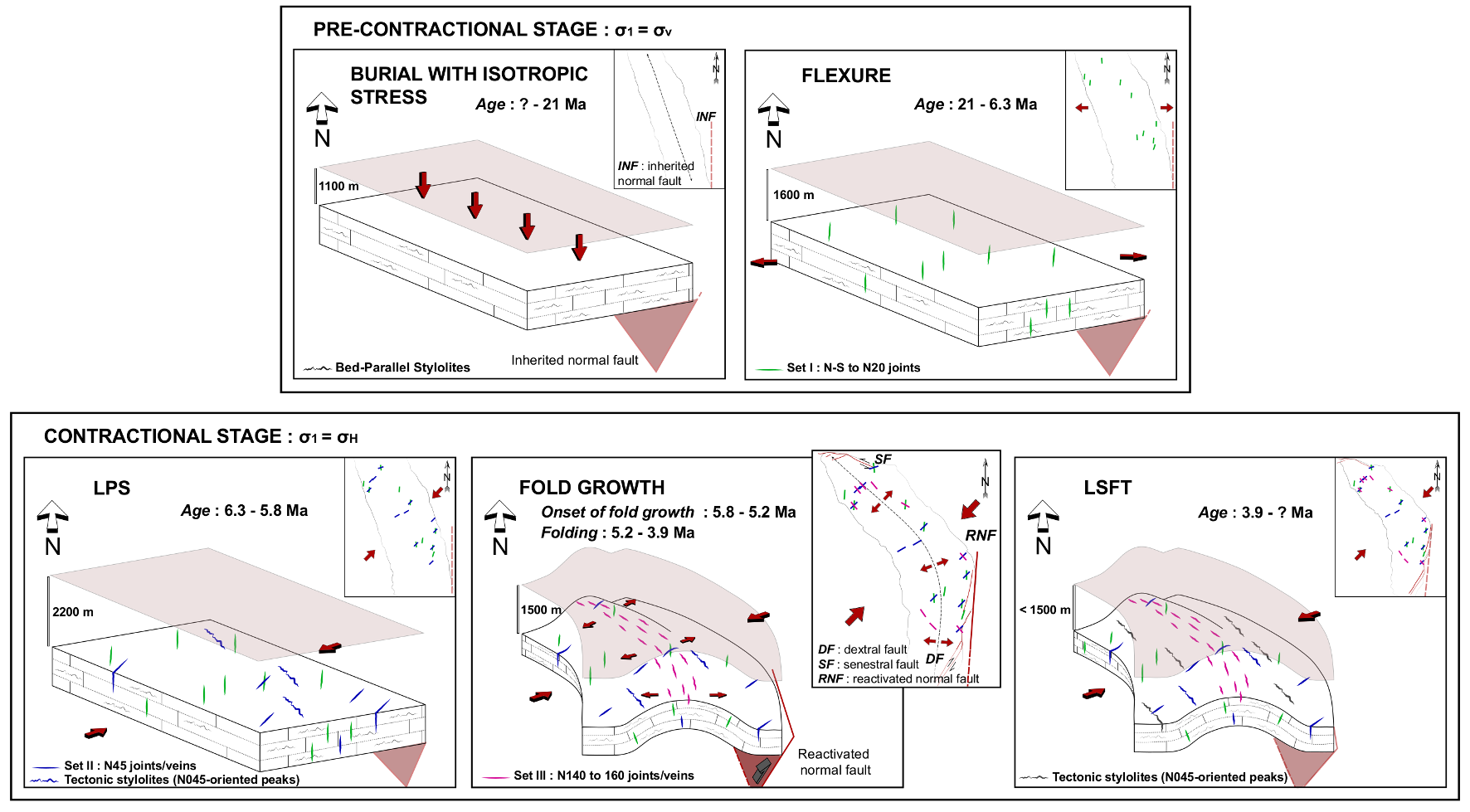
(ii)

this pre-contractional stage is partly coeval with an E-W extension related to the flexure of the Adriatic foreland [63,101], the onset of which is set to early Burdigalian (ca. 21 Ma, as defined by the inflection point of the burial curves), and which ended by middle Messinian (ca. 6.3 Ma, Figure 8). This E-W extension would be at the origin of the development of a network of N-S fractures (set I). Pre-folding N-S striking joints have already been described in this anticline [61], and in other anticlines, Monte Nero [121] and Monte Catria [66], without being related to regional extension. In the Conero anticline, however, [68] related a set of N-S, high angle to bedding, joints and veins associated with normal faults to a flexural event. Further considerations provide the existence of polyphase syndepositional normal faulting: the Barremian [146,147,148] and late Cretaceous phases of stretching (e.g., [95,149,150], well known in the Umbria-Marche-Sabina area, could have developed set I joints in the Maiolica and Scaglia Rossa, as well as the development of stylolites in the Mesozoic rocks.

(iii)

LPS stage, a pre/early-folding compressional stage with σ₁ NE-SW-oriented related to the Apenninic contraction [66,97,98,99]. The onset of this stage corresponds to the switch from formerly vertical to horizontal σ₁, associated with a N045 compression marked by the fractures and stylolites of set II. This stage of deformation is consistent regionally as it has been documented in the Monte Nero [121], Conero [68], and Monte Catria [66] anticlines, and identified in numerous folds of the UMAR [52,54]. Based on T₄₇ precipitation temperature and burial history, the LPS stage started since the middle Messinian (ca. 6.3 Ma). It has been reported in other case studies that the fold growth and associated underlying ramp activation is likely to be responsible for the uplift we reconstructed ca. 5.8 Ma [60]. Thus, we consider the LPS stage to have lasted from 6.3 Ma to 5.8 Ma;

(iv)

fold growth stage, characterized by a compression parallel to regional shortening, i.e., NE-SW-oriented [29] and local extension perpendicular to fold axis and related with strata curvature at fold hinge [60]. Based on the dating of the LPS, fold growth started at 5.8 Ma yet the T₄₇ points towards a related N135 striking joints/veins development during the latest Neogene-early Pliocene (ca. 5.2 to 3.9 Ma, Figure 8). That difference in timing suggests a 0.6 My long fault activity and strata tilting before curvature became high enough to developed outer-arc extension fractures;

(v)

LSFT, post-dating the fold growth stage and still associated with a NE-SW contractional trend. At this stage shortening is no longer accommodated by e.g., limb rotation [60] and is associated with tectonic stylolites with N045-oriented peaks. The E-W fractures locally measured cannot be associated with this deformation stage, because no consistent chronological relationships with the syn-folding fracture sets were identified. Isotopic analyses (Figure 8) suggest the onset of the LSFT by the Pliocene (ca. 3.9 Ma). Despite the record of recent seismic activity in this northern part of the Apennines, linked to a post-orogenic NE-SW extension [151], the end of this deformation stage can precisely be determined neither from previous studies carried out in Cingoli [61] nor from data collected during this study.

This deformation scenario is in line to the one proposed by [61], that discriminates seven sets of stylolites, of which complexity can be related to more local effect of the fold evolution.

The fold growth duration in Cingoli as constrained by the above results (ca. 1.9 My, from 5.8 to 3.9 Ma) is consistent with that established by [62] using the age of foredeep deposits. The age of the end of the foreland flexure, evaluated at ca. 6.3 Ma in our study, is also consistent within uncertainties with the early Messinian age (ca. 7.2–6.5 Ma) derived from the sedimentary dating of the flexure-related normal faults [63,64]. The abrupt increase in the slope of the burial curves (Figure 6) likely reflects the initiation of this flexure at about 21 Ma, which is older than the late Burdigalian (ca. 16 Ma) age previously proposed on the basis of the distribution and variations in thickness of the Schlier (Aquitanian-Serravallian) marking the deepening of the basin [63], and older than Serravallian (ca. 13.8 Ma) proposed at the west of the Cingoli Anticline, in the western part of the belt [79]. The horizontal isotropy of the compaction-related sedimentary stylolites, along which dissolution was active until 7 Ma, however, suggests a very limited imprint of the flexure on the magnitude of the horizontal stresses in the Cretaceous-Paleogene rocks until the early Messinian, when the flexure became important enough to cause fractures and large-scale normal faults [63].

The folding duration, estimated in our work at ~2 My (from 5.8 to 3.9 Ma) is consistent with the results of previous studies carried out in the more internal areas of the belt, using absolute dating methods to reconstruct the duration and timing of the deformations [60,71]: the difference in timing is in line with [62], and the duration of the folding is consistent with [60,71], which respectively dated the folding from 8 to 5 Ma [60], and from 9 to 7 Ma [71] (i.e., a duration of 2 to 3 My).

This case study illustrates the potential of the combination of mesostructural, paleopiezometric, and isotopic analyses, which reveals a regionally consistent sequence and timing of deformation stages, despite multiple sources of uncertainties. Namely, the refining of the timing of the flexure expression on the sedimentary reservoir is an example of how the study of mesostructures can provide insights on the large-scale structures. Another example of such upscaling lies in the interpretation of the arcuate shape of the Cingoli Anticline, that the distribution and timing of LPS related veins (set II) bounds to be a primary feature of the fold development, likely linked to the reactivation of an inherited N-S normal fault during folding (Figure 8).

7. Conclusions

This work, focused on the Cingoli Anticline in eastern UMAR, shows how the burial-deformation history of folded rocks can be unraveled using an original combination of ubiquitous features of carbonate rocks: fracture analysis, BPS paleopiezometry and vein cement geochemistry. The main conclusions are:

-

different stages of deformation were recognized: (i) E-W extension related to foreland flexure (σ₁ vertical); (ii) N045 oriented LPS; (iii) fold growth; (iv) LSFT, under a horizontal N045 contraction. Mesostructural analyses also support that the arcuate geometry of the Cingoli Anticline is a primary feature, probably linked to the oblique reactivation of a N-S inherited normal fault.

-

the burial history of strata was reconstructed with high resolution using roughness inversion applied to sedimentary stylolites. Our results highlight that this paleopiezometric technique yields consistent maximum depth estimates down to 2500 m, in agreement with previous studies in the western part of the UMAR.

-

the timing of deformation, and particularly the duration of the Apenninic contractional stages, was reconstructed from combined paleopiezometric, isotopic and mesostructral data. Following foreland flexure (ca. 21.2 to 6.3 Ma), LPS was dated from middle Messinian to early Pliocene (ca. 6.3 to 5.8 Ma) and fold growth occurred between early and middle Pliocene (ca. 5.8 to 3.9 Ma). The precise duration of LSFT remains out of reach. The duration of the fold growth phase is in line with previous estimates based on other proxies such as K-Ar and U-Pb absolute dating [71].

-

the O and C stable isotope signatures and clumped isotopes of ∆₄₇ of vein cements imply that the paleofluid system that prevailed during LPS and folding in this structure involve marine local fluids with limited interaction with the host rock, in agreement with earlier findings in the eastern UMAR.

Beyond regional implications, this study demonstrates the high potential of our new approach combining paleopiezometric, isotopic, and mesostructural data to reconstruct the sequence and to constrain the timing not only of local mesoscale deformation, but also of regional tectonic events in an orogenic system. Our results further confirm that the paleopiezometric inversion of the roughness of sedimentary stylolites for the vertical stresses is a reliable and powerful tool to unravel the amount and timing of burial without any assumption about the past geothermal gradient.

References

- Barton, C.A.; Zoback, M.D. Stress perturbations associated with active faults penetrated by boreholes: Possible evidence for near-complete stress drop and a new technique for stress magnitude measurement. J. Geophys. Res. 1994, 99, 9373–9390. [Google Scholar] [CrossRef]
- Zoback, M.L.; Zoback, M.D. Chapter 24: Tectonic stress field of the continental United States. Mem. Geol. Soc. Am. 1989, 172, 523–539. [Google Scholar] [CrossRef]
- Sibson, R.H. Crustal stress, faulting and fluid flow. Geol. Soc. Spec. Publ. 1994, 78, 69–84. [Google Scholar] [CrossRef]
- Sanderson, D.J.; Zhang, X. Stress-controlled localization of deformation and fluid flow in fractured rocks. Geol. Soc. Spec. Publ. 2004, 231, 299–314. [Google Scholar] [CrossRef]
- Sanderson, D.J.; Zhang, X. Critical stress localization of flow associated with deformation of well-fractured rock masses, with implications for mineral deposits. Geol. Soc. Spec. Publ. 1999, 155, 69–81. [Google Scholar] [CrossRef]
- Mourgues, R.; Gressier, J.B.; Bodet, L.; Bureau, D.; Gay, A. “Basin scale” versus “localized” pore pressure/stress coupling—Implications for trap integrity evaluation. Mar. Pet. Geol. 2011, 28, 1111–1121. [Google Scholar] [CrossRef]
- Beaudoin, N.; Lacombe, O. Recent and future trends in paleopiezometry in the diagenetic domain: Insights into the tectonic paleostress and burial depth history of fold-and-thrust belts and sedimentary basins. J. Struct. Geol. 2018, 114, 357–365. [Google Scholar] [CrossRef]
- Tavani, S.; Storti, F.; Lacombe, O.; Corradetti, A.; Muñoz, J.A.; Mazzoli, S. A review of deformation pattern templates in foreland basin systems and fold-and-thrust belts: Implications for the state of stress in the frontal regions of thrust wedges. Earth-Sci. Rev. 2015, 141, 82–104. [Google Scholar] [CrossRef]
- Bergbauer, S.; Pollard, D.D. A new conceptual fold-fracture model including prefolding joints, based on the Emigrant Gap anticline, Wyoming. Bull. Geol. Soc. Am. 2004, 116, 294–307. [Google Scholar] [CrossRef]
- Bellahsen, N.; Fiore, P.; Pollard, D.D. The role of fractures in the structural interpretation of Sheep Mountain Anticline, Wyoming. J. Struct. Geol. 2006, 28, 850–867. [Google Scholar] [CrossRef]
- La Bruna, V.; Lamarche, J.; Agosta, F.; Rustichelli, A.; Giuffrida,, A.; Salardon, R.; Marie, L. Structural Diagenesis, Early Embrittlement and Fracture Setting in Shallow-Water Platform Carbonates (Monte Alpi Southern Apennines, Italy). In Proceedings of the Fifth International Conference on Fault and Top Seals; European Association of Geoscientists & Engineers: Houten, The Netherlands, 2019; Volume 2019, pp. 1–5. [Google Scholar]
- Rocher, M.; Lacombe, O.; Angelier, J.; Chen, H.W. Mechanical twin sets in calcite as markers of recent collisional events in a fold-and-thrust belt: Evidence from the reefal limestones of southwestern Taiwan. Tectonics 1996, 15, 984–996. [Google Scholar] [CrossRef] [Green Version]
- Lacombe, O.; Angelier, J.; Rocher, M.; Bergues, J.; Deffontaines, B.; Chu, H.T.; Hu, J.C.; Lee, J.C. Stress patterns associated with folding at the front of a collision belt: Example from the Pliocene reef limestones of Yutengping (Taiwan). Bull. Soc. Geol. Fr. 1996, 167, 361–374. [Google Scholar]
- Rocher, M.; Lacombe, O.; Angelier, J.; Deffontaines, B.; Verdier, F. Cenozoic folding and faulting in the south Aquitaine Basin (France): Insights from combined structural and paleostress analyses. J. Struct. Geol. 2000, 22, 627–645. [Google Scholar] [CrossRef]
- Amrouch, K.; Lacombe, O.; Bellahsen, N.; Daniel, J.M.; Callot, J.P. Stress and strain patterns, kinematics and deformation mechanisms in a basement-cored anticline: Sheep Mountain Anticline, Wyoming. Tectonics 2010, 29. [Google Scholar] [CrossRef] [Green Version]
- Amrouch, K.; Beaudoin, N.; Lacombe, O.; Bellahsen, N.; Daniel, J.M. Paleostress magnitudes in folded sedimentary rocks. Geophys. Res. Lett. 2011, 38. [Google Scholar] [CrossRef] [Green Version]
- Callot, J.P.; Breesch, L.; Guilhaumou, N.; Roure, F.; Swennen, R.; Vilasi, N. Paleo-fluids characterisation and fluid flow modelling along a regional transect in Northern United Arab Emirates (UAE). Arab. J. Geosci. 2010, 3, 413–437. [Google Scholar] [CrossRef] [Green Version]
- Sassi, W.; Guiton, M.L.E.; Leroy, Y.M.; Daniel, J.M.; Callot, J.P. Constraints on bed scale fracture chronology with a FEM mechanical model of folding: The case of Split Mountain (Utah, USA). Tectonophysics 2012, 576–577, 197–215. [Google Scholar] [CrossRef]
- Smart, K.J.; Ferrill, D.A.; Morris, A.P.; McGinnis, R.N. Geomechanical modeling of stress and strain evolution during contractional fault-related folding. Tectonophysics 2012, 576–577, 171–196. [Google Scholar] [CrossRef]
- Beaudoin, N.; Bellahsen, N.; Lacombe, O.; Emmanuel, L. Fracture-controlled paleohydrogeology in a basement-cored, fault-related fold: Sheep Mountain Anticline, Wyoming, United States. Geochem. Geophys. Geosyst. 2011, 12. [Google Scholar] [CrossRef] [Green Version]
- Saintot, A.; Stephenson, R.; Brem, A.; Stovba, S.; Privalov, V. Paleostress field reconstruction and revised tectonic history of the Donbas fold and thrust belt (Ukraine and Russia). Tectonics 2003, 22. [Google Scholar] [CrossRef] [Green Version]
- Laubach, S.E.; Olson, J.E.; Gale, J.F.W. Are open fractures necessarily aligned with maximum horizontal stress? Earth Planet. Sci. Lett. 2004, 222, 191–195. [Google Scholar] [CrossRef]
- Bellahsen, N.; Fiore, P.E.; Pollard, D.D. From spatial variation of fracture patterns to fold kinematics: A geomechanical approach. Geophys. Res. Lett. 2006, 33. [Google Scholar] [CrossRef]
- Cooper, S.P.; Goodwin, L.B.; Lorenz, J.C. Fracture and fault patterns associated with basement-cored anticlines: The example of Teapot Dome, Wyoming. Am. Assoc. Pet. Geol. Bull. 2006, 90, 1903–1920. [Google Scholar] [CrossRef]
- Ahmadhadi, F.; Lacombe, O.; Daniel, J.-M. Early Reactivation of Basement Faults in Central Zagros (SW Iran): Evidence from Pre-folding Fracture Populations in Asmari Formation and Lower Tertiary Paleogeography. In Thrusts Belts and Foreland Basins. Frontiers in Earth Sciences; Lacombe, O., Roure, F., Vergés, J., Eds.; Springer: Berlin/Heidelberg, Germany, 2007; pp. 205–228. [Google Scholar]
- Ahmadhadi, F.; Daniel, J.M.; Azzizadeh, M.; Lacombe, O. Evidence for pre-folding vein development in the Oligo-Miocene Asmari Formation in the Central Zagros Fold Belt, Iran. Tectonics 2008, 27. [Google Scholar] [CrossRef] [Green Version]
- Lacombe, O.; Bellahsen, N.; Mouthereau, F. Fracture patterns in the Zagros Simply Folded Belt (Fars, Iran): Constraints on early collisional tectonic history and role of basement faults. Geol. Mag. 2011, 148, 940–963. [Google Scholar] [CrossRef]
- Casini, G.; Gillespie, P.A.; Vergés, J.; Romaire, I.; Fernández, N.; Casciello, E.; Saura, E.; Mehl, C.; Homke, S.; Embry, J.C.; et al. Sub-seismic fractures in foreland fold and thrust belts: Insight from the Lurestan Province, Zagros Mountains, Iran. Pet. Geosci. 2011, 17, 263–282. [Google Scholar] [CrossRef] [Green Version]
- Tavani, S.; Storti, F.; Baus, J.; Muoz, J.A. Late thrusting extensional collapse at the mountain front of the northern Apennines (Italy). Tectonics 2012, 31. [Google Scholar] [CrossRef]
- Beaudoin, N.; Leprêtre, R.; Bellahsen, N.; Lacombe, O.; Amrouch, K.; Callot, J.P.; Emmanuel, L.; Daniel, J.M. Structural and microstructural evolution of the Rattlesnake Mountain Anticline (Wyoming, USA): New insights into the Sevier and Laramide orogenic stress build-up in the Bighorn Basin. Tectonophysics 2012, 576–577, 20–45. [Google Scholar] [CrossRef]
- Stearns, D.W.; Friedman, M. Reservoirs in Fractured Rock. In Stratigraphic Oil and Gas Fields—Classification, Exploration Methods, and Case Histories. In Stratigraphic Oil and Gas Fields—Classification, Exploration Methods, and Case Histories; AAPG Special Volumes; Goud, H.R., Ed.; The American Association of petroleum Geologist: Tulsa, OK, USA, 1972; Volume 10, pp. 82–106. [Google Scholar]
- Engelder, T. Joints and Shear Fractures in Rock; Department of Geoscience, Pennsylvania State University: State College, PA, USA, 1987; pp. 27–69. ISBN 0-12-066265-5. [Google Scholar]
- Laubach, S.E. Subsurface fractures and their relationship to stress history in East Texas basin sandstone. Tectonophysics 1988, 156, 37–49. [Google Scholar] [CrossRef]
- Laubach, S.E. Paleostress directions from the preferred orientation of closed microfractures (fluid-inclusion planes) in sandstone, East Texas basin, U.S.A. J. Struct. Geol. 1989, 11, 603–611. [Google Scholar] [CrossRef]
- Fischer, M.P.; Woodward, N.B.; Mitchell, M.M. The kinematics of break-thrust folds. J. Struct. Geol. 1992, 14, 451–460. [Google Scholar] [CrossRef]
- Cooke, M.L. Fracture localization along faults with spatially varying friction. J. Geophys. Res. Solid Earth 1997, 102, 22425–22434. [Google Scholar] [CrossRef]
- Aldega, L.; Carminati, E.; Scharf, A.; Mattern, F.; Al-Wardi, M. Estimating original thickness and extent of the Semail Ophiolite in the eastern Oman Mountains by paleothermal indicators. Mar. Pet. Geol. 2017, 84, 18–33. [Google Scholar] [CrossRef]
- Aldega, L.; Bigi, S.; Carminati, E.; Trippetta, F.; Corrado, S.; Kavoosi, M.A. The Zagros fold-and-thrust belt in the Fars province (Iran): II. Thermal evolution. Mar. Pet. Geol. 2018, 93, 376–390. [Google Scholar] [CrossRef]
- Balestra, M.; Corrado, S.; Aldega, L.; Morticelli, M.G.; Sulli, A.; Rudkiewicz, J.-L.; Sassi, W. Thermal and structural modeling of the Scillato wedge-top basin source-to-sink system: Insights into the Sicilian fold-and-thrust belt evolution (Italy). Bulletin 2019, 131, 1763–1782. [Google Scholar] [CrossRef]
- Anders, M.H.; Laubach, S.E.; Scholz, C.H. Microfractures: A review. J. Struct. Geol. 2014, 69, 377–394. [Google Scholar] [CrossRef] [Green Version]
- Becker, S.P.; Eichhubl, P.; Laubach, S.E.; Reed, R.M.; Lander, R.H.; Bodnar, R.J. A 48 m.y. history of fracture opening, temperature, and fluid pressure: Cretaceous Travis Peak Formation, East Texas basin. Bull. Geol. Soc. Am. 2010, 122, 1081–1093. [Google Scholar] [CrossRef]
- Laubach, S.E.; Fall, A.; Copley, L.K.; Marrett, R.; Wilkins, S.J. Fracture porosity creation and persistence in a basement-involved Laramide fold, Upper Cretaceous Frontier Formation, Green River Basin, USA. Geol. Mag. 2016, 153, 887–910. [Google Scholar] [CrossRef] [Green Version]
- Fall, A.; Eichhubl, P.; Cumella, S.P.; Bodnar, R.J.; Laubach, S.E.; Becker, S.P. Testing the basin-centered gas accumulation model using fluid inclusion observations:Southern Piceance Basin, Colorado. Am. Assoc. Pet. Geol. Bull. 2012, 96, 2297–2318. [Google Scholar] [CrossRef]
- Lespinasse, M. Are fluid inclusion planes useful in structural geology? J. Struct. Geol. 1999, 21, 1237–1243. [Google Scholar] [CrossRef]
- Corrado, S.; Invernizzi, C.; Aldega, L.; D’errico, M.; Di Leo, P.; Mazzoli, S.; Zattin, M. Testing the validity of organic and inorganic thermal indicators in different tectonic settings from continental subduction to collision: The case history of the Calabria–Lucania border (southern Apennines, Italy). J. Geol. Soc. London. 2010, 167, 985–999. [Google Scholar] [CrossRef]
- Schito, A.; Andreucci, B.; Aldega, L.; Corrado, S.; Di Paolo, L.; Zattin, M.; Szaniawski, R.; Jankowski, L.; Mazzoli, S. Burial and exhumation of the western border of the Ukrainian Shield (Podolia): A multi-disciplinary approach. Basin Res. 2018, 30, 532–549. [Google Scholar] [CrossRef] [Green Version]
- Beaudoin, N.; Lacombe, O.; Roberts, N.M.W.; Koehn, D. U-Pb dating of calcite veins reveals complex stress evolution and thrust sequence in the Bighorn Basin, Wyoming, USA. Geology 2018, 46, 1015–1018. [Google Scholar] [CrossRef]
- Hoareau, G.; Claverie, F.; Pécheyran, C.; Paroissin, C.; Grignard, P.-A.; Motte, G.; Chailan, O.; Girard, J.-P. Direct U-Pb dating of carbonates from micron-scale femtosecond laser ablation inductively coupled plasma mass spectrometry images using robust regression. Geochronology 2021, 3, 67–87. [Google Scholar] [CrossRef]
- Aldega, L.; Viola, G.; Casas-Sainz, A.; Marcén, M.; Román-Berdiel, T.; Lelij, R. Unraveling Multiple Thermotectonic Events Accommodated by Crustal-Scale Faults in Northern Iberia, Spain: Insights From K-Ar Dating of Clay Gouges. Tectonics 2019, 38, 3629–3651. [Google Scholar] [CrossRef]
- Hoareau, G.; Crognier, N.; Lacroix, B.; Aubourg, C.; Roberts, N.M.W.; Niemi, N.; Branellec, M.; Beaudoin, N.; Ruiz, I.S. Combination of Δ47 and U-Pb dating in tectonic calcite veins unravel the last pulses related to the Pyrenean Shortening (Spain). Earth Planet. Sci. Lett. 2021, 553, 116636. [Google Scholar] [CrossRef]
- Mangenot, X.; Bonifacie, M.; Gasparrini, M.; Götz, A.; Chaduteau, C.; Ader, M.; Rouchon, V. Coupling Δ47 and fluid inclusion thermometry on carbonate cements to precisely reconstruct the temperature, salinity and δ18O of paleo-groundwater in sedimentary basins. Chem. Geol. 2017, 472, 44–57. [Google Scholar] [CrossRef]
- Renard, F.; Schmittbuhl, J.; Gratier, J.P.; Meakin, P.; Merino, E. Three-dimensional roughness of stylolites in limestones. J. Geophys. Res. 2004, 109. [Google Scholar] [CrossRef] [Green Version]
- Schmittbuhl, J.; Renard, F.; Gratier, J.P.; Toussaint, R. Roughness of stylolites: Implications of 3D high resolution topography measurements. Phys. Rev. Lett. 2004, 93, 238501. [Google Scholar] [CrossRef] [Green Version]
- Ebner, M.; Piazolo, S.; Renard, F.; Koehn, D. Stylolite interfaces and surrounding matrix material: Nature and role of heterogeneities in roughness and microstructural development. J. Struct. Geol. 2010, 32, 1070–1084. [Google Scholar] [CrossRef]
- Ebner, M.; Toussaint, R.; Schmittbuhl, J.; Koehn, D.; Bons, P. Anisotropic scaling of tectonic stylolites: A fossilized signature of the stress field? J. Geophys. Res. 2010, 115, B06403. [Google Scholar] [CrossRef] [Green Version]
- Rolland, A.; Toussaint, R.; Baud, P.; Schmittbuhl, J.; Conil, N.; Koehn, D.; Renard, F.; Gratier, J. Modeling the growth of stylolites in sedimentary rocks. J. Geophys. Res. Solid Earth 2012, 117, B6. [Google Scholar] [CrossRef] [Green Version]
- Rolland, A.; Toussaint, R.; Baud, P.; Conil, N.; Landrein, P. Morphological analysis of stylolites for paleostress estimation in limestones. Int. J. Rock Mech. Min. Sci. 2014, 67, 212–225. [Google Scholar] [CrossRef] [Green Version]
- Koehn, D.; Rood, M.P.; Beaudoin, N.; Chung, P.; Bons, P.D.; Gomez-Rivas, E. A new stylolite classification scheme to estimate compaction and local permeability variations. Sediment. Geol. 2016, 346, 60–71. [Google Scholar] [CrossRef] [Green Version]
- Bertotti, G.; de Graaf, S.; Bisdom, K.; Oskam, B.; Vonhof, H.B.; Bezerra, F.H.R.; Reijmer, J.J.G.; Cazarin, L.C. Fracturing and fluid-flow during post-rift subsidence in carbonates of the Jandaíra Formation, Potiguar Basin, NE Brazil. Basin Res. 2017, 29, 836–853. [Google Scholar] [CrossRef] [Green Version]
- Beaudoin, N.; Labeur, A.; Lacombe, O.; Koehn, D.; Billi, A.; Hoareau, G.; Boyce, A.; John, C.M.; Marchegiano, M.; Roberts, N.M.; et al. Regional-scale paleofluid system across the Tuscan Nappe–Umbria Marche Arcuate Ridge (northern Apennines) as revealed by mesostructural and isotopic analyses of stylolite-vein networks. Solid Earth 2020, 11, 1617–1641. [Google Scholar] [CrossRef]
- Petracchini, L.; Antonellini, M.; Billi, A.; Scrocca, D. Fault development through fractured pelagic carbonates of the Cingoli anticline, Italy: Possible analog for subsurface fluid-conductive fractures. J. Struct. Geol. 2012, 45, 21–37. [Google Scholar] [CrossRef]
- Calamita, F.; Cello, G.; Deiana, G.; Paltrinieri, W. Structural styles, chronology rates of deformation, and time-space relationships in the Umbria-Marche thrust system (central Apennines, Italy). Tectonics 1994, 13, 873–881. [Google Scholar] [CrossRef]
- Mazzoli, S.; Deiana, G.; Galdenzi, S.; Cello, G. Miocene fault-controlled sedimentation and thrust propagation in the previously faulted external zones of the Umbria-Marche Apennines, Italy. EGU Stephan Mueller Spec. Publ. Ser. 2002, 1, 195–209. [Google Scholar] [CrossRef]
- Calamita, F.; Cello, G.; Invernizzi, C.; Paltrinieri, W. Stile strutturale e crono- logia della deformazione lungo la traversa M. S. Vicino. Stud. Geol. Camerti 1990, 69–86. [Google Scholar] [CrossRef]
- Caricchi, C.; Aldega, L.; Corrado, S. Reconstruction of maximum burial along the Northern Apennines thrust wedge (Italy) by indicators of thermal exposure and modeling. Bull. Geol. Soc. Am. 2015, 127, 428–442. [Google Scholar] [CrossRef]
- Tavani, S.; Storti, F.; Salvini, F.; Toscano, C. Stratigraphic versus structural control on the deformation pattern associated with the evolution of the Mt. Catria anticline, Italy. J. Struct. Geol. 2008, 30, 664–681. [Google Scholar] [CrossRef]
- Petracchini, L.; Antonellini, M.; Billi, A.; Scrocca, D. Syn-thrusting polygonal normal faults exposed in the hinge of the Cingoli anticline, northern Apennines, Italy. Front. Earth Sci. 2015, 3, 67. [Google Scholar] [CrossRef] [Green Version]
- Díaz General, E.N.; Mollema, P.N.; Antonellini, M. Fracture patterns and fault development in the pelagic limestones of the Monte Conero anticline (Italy). Ital. J. Geosci. 2015, 134, 495–512. [Google Scholar] [CrossRef]
- Calamita, F.; Coppola, L.; Deiana, G.; Ivernizzi, C.; Mastrovincenzo, S. Le associazioni strutturali di Genge e M. Rotondo; un motivo ricorrente nella thrust belt umbro-marchigiana settentrionale. Boll. Della Soc. Geol. Ital. 1987, 106, 141–151. [Google Scholar]
- Invernizzi, C. Low temperature deformation in naturally deformed marly limestones from the Umbria-Marche Apennines. Ann. Tectonicae 1994, 8, 119–133. [Google Scholar]
- Curzi, M.; Aldega, L.; Bernasconi, S.M.; Berra, F.; Billi, A.; Boschi, C.; Franchini, S.; Van der Lelij, R.; Viola, G.; Carminati, E. Architecture and evolution of an extensionally-inverted thrust (Mt. Tancia Thrust, Central Apennines): Geological, structural, geochemical, and K–Ar geochronological constraints. J. Struct. Geol. 2020, 136, 104059. [Google Scholar] [CrossRef]
- Lavecchia, G.; Minelli, G.; Pialli, G. The Umbria-Marche arcuate fold belt (Italy). Tectonophysics 1988, 146, 125–137. [Google Scholar] [CrossRef]
- Elter, F.M.; Elter, P.; Eva, C.; Eva, E.; Kraus, R.K.; Padovano, M.; Solarino, S. An alternative model for the recent evolution of the Northern-Central Apennines (Italy). J. Geodyn. 2012, 54, 55–63. [Google Scholar] [CrossRef]
- Tozer, R.S.J.; Butler, R.W.H.; Corrado, S. Comparing thin- and thick-skinned thrust tectonic models of the Central Apennines, Italy. Stephan Mueller Spec. Publ. Ser. 2002, 1, 181–194. [Google Scholar] [CrossRef]
- Scisciani, V.; Agostini, S.; Calamita, F.; Pace, P.; Cilli, A.; Giori, I.; Paltrinieri, W. Positive inversion tectonics in foreland fold-and-thrust belts: A reappraisal of the Umbria-Marche Northern Apennines (Central Italy) by integrating geological and geophysical data. Tectonophysics 2014, 637, 218–237. [Google Scholar] [CrossRef]
- Mazzoli, S.; Aldega, L.; Corrado, S.; Invernizzi, C.; Zattin, M. Pliocene-quaternary thrusting, syn-orogenic extension and tectonic exhumation in the Southern Apennines (Italy): Insights from the Monte Alpi area. Spec. Pap. Soc. Am. 2006, 414, 55. [Google Scholar]
- Boccaletti, M.; Calamita, F.; Viandante, M.G. The lithospheric Apennine Neo-Chain developing since the Lower Pliocene as a result of the Africa-Europe convergence. Boll. della Soc. Geol. Ital. 2005, 124, 87–105. [Google Scholar]
- Satolli, S.; Pace, P.; Viandante, M.; Calamita, F. Lateral variations in tectonic style across cross-strike discontinuities: An example from the Central Apennines belt (Italy). Int. J. Earth Sci. 2014, 103, 2301–2313. [Google Scholar] [CrossRef]
- Brozzetti, F.; Cirillo, D.; Luchetti, L. Timing of Contractional Tectonics in the Miocene Foreland Basin System of the Umbria Pre-Apennines (Italy): An Updated Overview. Geosciences 2021, 11, 97. [Google Scholar] [CrossRef]
- Cello, G.; Mazzoli, S.; Tondi, E.; Turco, E. Active tectonics in the central Apennines and possible implications for seismic hazard analysis in peninsular Italy. Tectonophysics 1997, 272, 43–68. [Google Scholar] [CrossRef]
- Ghisetti, F.; Vezzani, L. Normal faulting, extension and uplift in the outer thrust belt of the central Apennines (Italy): Role of the Caramanico fault. Basin Res. 2002, 14, 225–236. [Google Scholar] [CrossRef]
- Santantonio, M. Pelagic carbonate platforms in the geologic record: Their classification and sedimentary and paleotectonic evolution. Am. Assoc. Pet. Geol. Bull. 1994, 78, 122–141. [Google Scholar] [CrossRef]
- Santantonio, M. Facies associations and evolution of pelagic carbonate platform/basin systems: Examples from the Italian Jurassic. Sedimentology 1993, 40, 1039–1067. [Google Scholar] [CrossRef]
- Carminati, E.; Lustrino, M.; Cuffaro, M.; Doglioni, C. Tectonics, magmatism and geodynamics of Italy: What we know and what we imagine. J. Virtual Explor. 2010, 36, 10–3809. [Google Scholar] [CrossRef]
- Bigi, S.; Milli, S.; Corrado, S.; Casero, P.; Aldega, L.; Botti, F.; Moscatelli, M.; Stanzione, O.; Falcini, F.; Marini, M.; et al. Stratigraphy, structural setting and burial history of the Messinian Laga basin in the context of Apennine foreland basin system. J. Mediterr. Earth Sci. 2009, 1, 61–84. [Google Scholar] [CrossRef]
- Bally, A.W.; Burbi, W.; Cooper, J.C.; Ghelardoni, L. Balanced sections and seismic reflection profiles across the Central Apennines. Mem. Soc. Geol. Ital. 1986, 107, 109–130. [Google Scholar]
- Ghisetti, F.; Vezzani, L. Geometric and kinematic complexities in the Marche-Abruzzi external zones (Central Apennines, Italy). Geol. Rundschau 1988, 77, 63–78. [Google Scholar] [CrossRef]
- Hill, K.; Hayward, A. Structural constraints on the Tertiary plate tectonic evolution of Italy. Mar. Pet. Geol. 1988, 5, 2–16. [Google Scholar] [CrossRef]
- Lacombe, O.; Bellahsen, N. Thick-skinned tectonics and basement-involved fold–thrust belts: Insights from selected Cenozoic orogens. Geol. Mag. 2016, 153, 763–810. [Google Scholar] [CrossRef] [Green Version]
- Hippolyte, J.-C.; Angelier, J.; Barrier, E. Compressional and extensional tectonics in an arc system: Example of the Southern Apennines. J. Struct. Geol. 1995, 17, 1725–1740. [Google Scholar] [CrossRef]
- Mazzoli, S.; Cello, G.; Deiana, G.; Galdenzi, S.; Gambini, R.; Mancinelli, A.; Mattioni, L.; Shiner, P.; Tondi, E. Modes of foreland deformation ahead of the Apennine thrust front. J. Czech Geol. Soc. 2000, 45, 246. [Google Scholar]
- Scisciani, V.; Calamita, F.; Tavarnelli, E.; Rusciadelli, G.; Ori, G.-G.; Paltrinieri, W. Foreland-dipping normal faults in the iner edges of syn-orogenic basins: A case from the Central Apennines, Italy. Tectonophysics 2001, 330, 211–224. [Google Scholar] [CrossRef]
- Calamita, F.; Paltrinieri, W.; Pelorosso, M.; Scisciani, V.; Tavarnelli, E. Inherited Mesozoic architecture of the Adria continental palaeomargin in the neogene central apennines orogenic system, Italy. Boll. Della Soc. Geol. Ital. 2003, 122, 307–318. [Google Scholar]
- Rusciadelli, G.; Viandante, M.G.; Calamita, F.; Cook, A.C. Burial-exhumation history of the central Apennines (Italy), from the foreland to the chain building: Thermochronological and geological data. Terra Nov. 2005, 17, 560–572. [Google Scholar] [CrossRef]
- Tavarnelli, E. Ancient synsedimentary structural control on thrust ramp development: An example from the Northern Apennines, Italy. Terra Nov. 2007, 8, 65–74. [Google Scholar] [CrossRef]
- Pace, P.; Calamita, F. Push-up inversion structures v. fault-bend reactivation anticlines along oblique thrust ramps: Examples from the Apennines fold-and-thrust belt (Italy). J. Geol. Soc. Lond. 2014, 171, 227–238. [Google Scholar] [CrossRef]
- Marshak, S.; Geiser, P.A.; Alvarez, W.; Engelder, T. Mesoscopic fault array of the northern Umbrian Appennine fold belt, Italy: Geometry of conjugate shear by pressure-solution slip. Geol. Soc. Am. Bull. 1982, 93, 1013–1022. [Google Scholar] [CrossRef]
- Storti, F.; Rossetti, F.; Salvini, F. Structural architecture and displacement accomodation mechanisms at the termination of the Priestley Fault, northern Victoria Land, Antarctica. Tectonophysics 2001, 341, 141–161. [Google Scholar] [CrossRef]
- Barchi, M.; Alvarez, W.; Shimabukuro, D.H. The Umbria-Marche Apennines as a double orogen: Observations and hypotheses. Ital. J. Geosci. 2012, 131, 258–271. [Google Scholar] [CrossRef]
- Calamita, F.; Deiana, G. The arcuate shape of the Umbria-Marche-Sabina Apennines (Central Italy). Tectonophysics 1988, 146, 139–147. [Google Scholar] [CrossRef]
- Deiana, G.; Cello, G.; Chiocchini, M.; Galdenzi, S.; Mazzoli, S.; Pistolesi, E.; Potetti, M.; Romano, A.; Turco, E.; Principi, M. Tectonic evolution of the external zones of the Umbria-Marche Apennines in the Monte San Vicino-Cingoli area. Boll. Della Soc. Geol. Ital. 2002, 1, 229–238. [Google Scholar]
- Cita, M.B.; Abbate, E.; Ballini, M.; Conti, A.; Falorni, P.; Germani, D.; Petti, F.M. Carta Geologica d’Italia–1: 50.000, Catalogo delle Formazioni, Unità tradizionali. Quad. Serv. Geol. D’It. Ser. III 2007, 7, 382. [Google Scholar]
- Menichetti, M. La sezione geologica Cingoli—M. Maggio-Tevere nell’Appennino umbro-marchigiano: Analisi cinematica e strutturale. Stud. Geol. Camerti 1991, special vo, 315–328. [Google Scholar]
- Centamore, E.; Chiocchini, M.; Deiana, G.; Micarelli, A.; Pieruccini, U. Contributo alla conoscenda del Giurassico dell’Appennino Umbro-Marchigiano. Stud. Geol. Camerti 1971, 1, 7–89. [Google Scholar] [CrossRef]
- Farinacci, A. Jurassic Sediments in the Umbro-Marchean Apennines: An Alternative Model; Istituto di Geologia e Paleontologia: Roma, Italy, 1981. [Google Scholar]
- Santantonio, M.; Carminati, E. Jurassic rifting evolution of the Apennines and Southern Alps (Italy): Parallels and differences. Bulletin 2011, 123, 468–484. [Google Scholar] [CrossRef]
- Koehn, D.; Renard, F.; Toussaint, R.; Passchier, C.W. Growth of stylolite teeth patterns depending on normal stress and finite compaction. Earth Planet. Sci. Lett. 2007, 257, 582–595. [Google Scholar] [CrossRef] [Green Version]
- Toussaint, R.; Aharonov, E.; Koehn, D.; Gratier, J.P.; Ebner, M.; Baud, P.; Rolland, A.; Renard, F. Stylolites: A review. J. Struct. Geol. 2018, 114, 163–195. [Google Scholar] [CrossRef] [Green Version]
- Grohmann, C.H.; Campanha, G.A. OpenStereo: Open source, cross-platform software for structural geology analysis. AGU Fall Meet. Abstr. 2010, 2010, IN31C-06. [Google Scholar]
- Angelier, J. Tectonic analysis of fault slip data sets. J. Geophys. Res. 1984, 89, 5835–5848. [Google Scholar] [CrossRef]
- Lacombe, O. Do fault slip data inversions actually yield“ paleostresses” that can be compared with contemporary stresses? A critical discussion. Comptes Rendus-Geosci. 2012, 344, 159–173. [Google Scholar] [CrossRef]
- Aydin, A.; Basu, A. The Schmidt hammer in rock material characterization. Eng. Geol. 2005, 81, 1–14. [Google Scholar] [CrossRef]
- Katz, O.; Reches, Z.; Roegiers, J.-C. Evaluation of mechanical rock properties using a Schmidt Hammer. Int. J. Rock Mech. Min. Sci. 2000, 37, 723–728. [Google Scholar] [CrossRef]
- Ebner, M.; Koehn, D.; Toussaint, R.; Renard, F. The influence of rock heterogeneity on the scaling properties of simulated and natural stylolites. J. Struct. Geol. 2009, 31, 72–82. [Google Scholar] [CrossRef] [Green Version]
- Ebner, M.; Koehn, D.; Toussaint, R.; Renard, F.; Schmittbuhl, J. Stress sensitivity of stylolite morphology. Earth Planet. Sci. Lett. 2009, 277, 394–398. [Google Scholar] [CrossRef] [Green Version]
- Koehn, D.; Ebner, M.; Renard, F.; Toussaint, R.; Passchier, C.W. Modelling of stylolite geometries and stress scaling. Earth Planet. Sci. Lett. 2012, 341–344, 104–113. [Google Scholar] [CrossRef] [Green Version]
- Beaudoin, N.; Gasparrini, M.; David, M.E.; Lacombe, O.; Koehn, D. Bedding-parallel stylolites as a tool to unravel maximum burial depth in sedimentary basins: Application to Middle Jurassic carbonate reservoirs in the Paris basin, France. Bull. Geol. Soc. Am. 2019, 131, 1239–1254. [Google Scholar] [CrossRef]
- Beaudoin, N.; Lacombe, O.; David, M.E.; Koehn, D. Does stress transmission in forelands depend on structural style? Distinctive stress magnitudes during Sevier thin-skinned and Laramide thick-skinned layer-parallel shortening in the Bighorn Basin (USA) revealed by stylolite and calcite twinning paleopiez. Terra Nov. 2020, 32, 225–233. [Google Scholar] [CrossRef]
- Simonsen, I.; Hansen, A.; Nes, O.M. Determination of the Hurst exponent by use of wavelet transforms. Phys. Rev. 1998, 58, 2779–2787. [Google Scholar] [CrossRef] [Green Version]
- Wright, K.; Cygan, R.T.; Slater, B. Structure of the (1014) surfaces of calcite, dolomite and magnesite under wet and dry conditions. Phys. Chem. Chem. Phys. 2001, 3, 839–844. [Google Scholar] [CrossRef] [Green Version]
- Beaudoin, N.; Koehn, D.; Lacombe, O.; Lecouty, A.; Billi, A.; Aharonov, E.; Parlangeau, C. Fingerprinting stress: Stylolite and calcite twinning paleopiezometry revealing the complexity of progressive stress patterns during folding—The case of the Monte Nero anticline in the Apennines, Italy. Tectonics 2016, 34, 1687–1712. [Google Scholar] [CrossRef] [Green Version]
- Vass, A.; Koehn, D.; Toussaint, R.; Ghani, I.; Piazolo, S. The importance of fracture-healing on the deformation of fluid-filled layered systems. J. Struct. Geol. 2014, 67, 94–106. [Google Scholar] [CrossRef] [Green Version]
- Dietrich, D.; McKenzie, J.A.; Song, H. Origin of calcite in syntectonic veins as determined from carbon- isotope ratios. Geology 1983, 11, 547–551. [Google Scholar] [CrossRef]
- Shemesh, A.; Ron, H.; Erel, Y.; Kolodny, Y.; Nur, A. Isotopic composition of vein calcite and its fluid inclusions: Implication to paleohydrological systems, tectonic events and vein formation processes. Chem. Geol. 1992, 94, 307–314. [Google Scholar] [CrossRef]
- Templeton, A.S. Fluids and the Heart Mountain Fault revisited. Geology 1995, 23, 929–932. [Google Scholar] [CrossRef]
- Douglas, T.A.; Chamberlain, C.P.; Poage, M.A.; Abruzzese, M.; Shultz, S.; Henneberry, J.; Layer, P. Fluid flow and the heart mountain fault: A stable isotopic, fluid inclusion, and geochronologic study. Geofluids 2003, 3, 13–32. [Google Scholar] [CrossRef]
- Vilasi, N.; Malandain, J.; Barrier, L.; Callot, J.P.; Amrouch, K.; Guilhaumou, N.; Lacombe, O.; Muska, K.; Roure, F.; Swennen, R. From outcrop and petrographic studies to basin-scale fluid flow modelling: The use of the Albanian natural laboratory for carbonate reservoir characterisation. Tectonophysics 2009, 474, 367–392. [Google Scholar] [CrossRef]
- Barbier, M.; Hamon, Y.; Callot, J.P.; Floquet, M.; Daniel, J.M. Sedimentary and diagenetic controls on the multiscale fracturing pattern of a carbonate reservoir: The Madison Formation (Sheep Mountain, Wyoming, USA). Mar. Pet. Geol. 2012, 29, 50–67. [Google Scholar] [CrossRef]
- Gasparrini, M.; Lacombe, O.; Rohais, S.; Belkacemi, M.; Euzen, T. Natural mineralized fractures from the Montney-Doig unconventional reservoirs (Western Canada Sedimentary Basin): Timing and controlling factors. Mar. Pet. Geol. 2021, 124, 104826. [Google Scholar] [CrossRef]
- Bons, P.D.; Elburg, M.A.; Gomez-Rivas, E. A review of the formation of tectonic veins and their microstructures. J. Struct. Geol. 2012, 43, 33–62. [Google Scholar] [CrossRef]
- Daëron, M.; Blamart, D.; Peral, M.; Affek, H.P. Absolute isotopic abundance ratios and the accuracy of Δ47 measurements. Chem. Geol. 2016, 442, 83–96. [Google Scholar] [CrossRef]
- Bernasconi, S.M.; Müller, I.A.; Bergmann, K.D.; Breitenbach, S.F.M.; Fernandez, A.; Hodell, D.A.; Jaggi, M.; Meckler, A.N.; Millan, I.; Ziegler, M. Reducing uncertainties in carbonate clumped isotope analysis through consistent carbonate-based standardization. Geochem. Geophys. Geosyst. 2018, 19, 2895–2914. [Google Scholar] [CrossRef] [PubMed] [Green Version]
- Kim, S.T.; Mucci, A.; Taylor, B.E. Phosphoric acid fractionation factors for calcite and aragonite between 25 and 75 °C: Revisited. Chem. Geol. 2007, 246, 135–146. [Google Scholar] [CrossRef]
- Daëron, M. Full propagation of analytical uncertainties in D47 measurements. Geochem. Geophys. Geosyst. 2020, 1–26. [Google Scholar] [CrossRef]
- Kele, S.; Breitenbach, S.F.M.; Capezzuoli, E.; Meckler, A.N.; Ziegler, M.; Millan, I.M.; Kluge, T.; Deák, J.; Hanselmann, K.; John, C.M.; et al. Temperature dependence of oxygen- and clumped isotope fractionation in carbonates: A study of travertines and tufas in the 6-95°C temperature range. Geochim. Cosmochim. Acta 2015, 168, 172–192. [Google Scholar] [CrossRef]
- Cardozo, N. Backtrip: Performs 1D “Airy type” Backstripping of Sedimentary Strata. 2011. Available online: https://downloadsafer.com/software/osxbackstrip/ (accessed on 30 January 2021).
- Allen, P.A.; Allen, J.R. Basin Analysis: Principles and Aplications, Blackwell Scientific Publication, 1st ed.; Blackwell Scientific Publications: Oxford, UK; London, UK, 1990; ISBN 0632024224. [Google Scholar]
- Watts, A.B. Isostasy and Flexure of the Lithosphere; Paperback; Cambridge University Press: Cambridge, UK, 2001; ISBN 9780521006002. [Google Scholar]
- Beaudoin, N.; Bellahsen, N.; Lacombe, O.; Emmanuel, L.; Pironon, J. Crustal-scale fluid flow during the tectonic evolution of the Bighorn Basin (Wyoming, USA). Basin Res. 2014, 26, 403–435. [Google Scholar] [CrossRef] [Green Version]
- Aldega, L.; Botti, F.; Corrado, S. Clay mineral assemblages and vitrinite reflectance in the Laga Basin (Central Apennines, Italy): What do they record? Clays Clay Miner. 2007, 55, 504–518. [Google Scholar] [CrossRef]
- Kim, S.T.; O’Neil, J.R. Equilibrium and nonequilibrium oxygen isotope effects in synthetic carbonates. Geochim. Cosmochim. Acta 1997, 61, 3461–3475. [Google Scholar] [CrossRef]
- Di Naccio, D.; Boncio, P.; Cirilli, S.; Casaglia, F.; Morettini, E.; Lavecchia, G.; Brozzetti, F. Role of mechanical stratigraphy on fracture development in carbonate reservoirs: Insights from outcropping shallow water carbonates in the Umbria-Marche Apennines, Italy. J. Volcanol. Geotherm. Res. 2005, 148, 98–115. [Google Scholar] [CrossRef]
- Petit, J.; Barquins, M. Can natural faults propagate under mode II conditions? Tectonics 1988, 7, 1243–1256. [Google Scholar] [CrossRef]
- Homberg, C.; Hu, J.C.; Angelier, J.; Bergerat, F.; Lacombe, O. Characterization of stress perturbations near major fault zones: Insights from 2-D distinct-element numerical modelling and field studies (Jura mountains). J. Struct. Geol. 1997, 19, 703–718. [Google Scholar] [CrossRef]
- Beaudoin, N.; Lacombe, O.; Koehn, D.; David, M.E.; Farrell, N.; Healy, D. Vertical stress history and paleoburial in foreland basins unravelled by stylolite roughness paleopiezometry: Insights from bedding-parallel stylolites in the Bighorn Basin, Wyoming, USA. J. Struct. Geol. 2020, 136, 104061. [Google Scholar] [CrossRef]
- Fabbi, S.; Citton, P.; Romano, M.; Cipriani, A. Detrital events within pelagic deposits of the Umbria-Marche Basin (Northern Apennines, Italy): Further evidence of Early Cretaceous tectonics. J. Mediterr. Earth Sci. 2016, 8, 39–52. [Google Scholar]
- Cipriani, A.; Bottini, C. Early Cretaceous tectonic rejuvenation of an Early Jurassic margin in the Central Apennines: The “Mt. Cosce Breccia” . Sediment. Geol. 2019, 387, 57–74. [Google Scholar] [CrossRef]
- Cipriani, A.; Bottini, C. Unconformities, neptunian dykes and mass-transport deposits as an evidence for Early Cretaceous syn-sedimentary tectonics: New insights from the Central Apennines. Ital. J. Geosci. 2019, 138, 333–354. [Google Scholar] [CrossRef]
- Decandia, F.A. Geologia dei Monti di Spoleto (Provincia di Perugia). Boll. Della Soc. Geol. Ital. 1982, 101, 291–315. [Google Scholar]
- Marchegiani, L.; Bertotti, G.; Cello, G.; Deiana, G.; Mazzoli, S.; Tondi, E. Pre-orogenic tectonics in the Umbria-Marche sector of the Afro-Adriatic continental margin. Tectonophysics 1999, 315, 123–143. [Google Scholar] [CrossRef]
- Mazzoli, S.; Santini, S.; Macchiavelli, C.; Ascione, A. Active tectonics of the outer northern Apennines: Adriatic vs. Po Plain seismicity and stress fields. J. Geodyn. 2015, 84, 62–76. [Google Scholar] [CrossRef]