Article

A Comparison Study of Explicit and Implicit 3-D Transient Electromagnetic Forward Modeling Schemes on Multi-Resolution Grid

1
Department of Civil, Environmental and Natural Resources Engineering, Luleå University of Technology, 97187 Luleå, Sweden
2
Institute of Geophysics and Meteorology, University of Cologne, 50923 Cologne, Germany
3
College of Earth, Ocean and Atmospheric Sciences, Oregon State University, Corvallis, OR 97331, USA
*
Author to whom correspondence should be addressed.
Geosciences 2021, 11(6), 257; https://doi.org/10.3390/geosciences11060257
Submission received: 19 February 2021 / Revised: 23 April 2021 / Accepted: 8 June 2021 / Published: 15 June 2021
(This article belongs to the Special Issue 3D Modelling/Inversion for Mineral Exploration)

Abstract

:
This study compares the efficiency of 3-D transient electromagnetic forward modeling schemes on the multi-resolution grid for various modeling scenarios. We developed time-domain finite-difference modeling based on the explicit scheme earlier. In this work, we additionally implement 3-D transient electromagnetic forward modeling using the backward Euler implicit scheme. The iterative solver is used for solving the system of equations and requires a proper initial guess that has significant effect on the convergence. The standard approach usually employs the solution of a previous time step as an initial guess, which might be too conservative. Instead, we test various initial guesses based on the linear extrapolation or linear combination of the solutions from several previous steps. We build up the implicit scheme forward modeling on the multi-resolution grid, which allows for the adjustment of the horizontal resolution with depth, hence improving the performance of the forward operator. Synthetic examples show the implicit scheme forward modeling using the linearly combined initial guess estimate on the multi-resolution grid additionally reduces the run time compared to the standard initial guess approach. The result of comparison between the implicit scheme developed here with the previously developed explicit scheme shows that the explicit scheme modeling is more efficient for more conductive background models often found in environmental studies. However, the implicit scheme modeling is more suitable for the simulation with highly resistive background models, usually occurring in mineral exploration scenarios. Thus, the inverse problem can be solved using more efficient forward solution depending on the modeling setup and background resistivity.

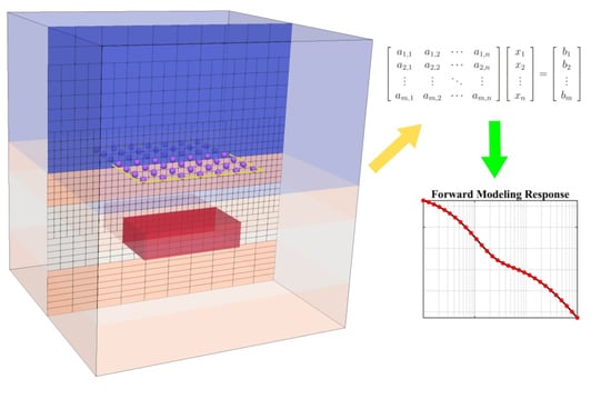
Graphical Abstract

1. Introduction

The transient electromagnetic (TEM) method is widely used in many geophysical applications, including exploration for minerals [1,2,3]. In order to fully exploit the observed data, the full 3-D quantitative data inversion is warranted. The inversion techniques rely heavily on accurate and efficient forward modeling algorithms.
The TEM forward modeling can be implemented in frequency-domain and thereafter transformed to time-domain using the Fourier transform. However, the frequency-domain approach generally requires a sufficiently dense and wide frequency range to ensure the accuracy of the solution [4]. Alternatively, the simulation can be implemented directly in the time-domain so that the electromagnetic (EM) fields are recursively advanced using time-stepping [5]. The time-domain TEM modeling can be further classified into explicit and implicit schemes, depending on how the time-stepping is approached.
The classical explicit scheme discretizes Maxwell equations directly in a leapfrog fashion. It involves lightweight computations in each time step, alternating between electric and magnetic fields from Ampere’s and Faraday’s laws, which are merely matrix-vector operations. However, the time-stepping is conditionally stable in that the length of the time step is constrained by the Courant–Friedrichs–Lewy (CFL) condition [6], i.e., the time that the EM wave spends to pass the minimum length of the model grid at light speed. This usually small time step needs to be fixed during the whole modeling process, which is impractical to implement for the time range of the TEM problem. Oristaglio and Hohmann [7] and Wang and Hohmann [8] applied a modified version of the Du Fort-Frankel method, which replaces the displacement currents term with a variable artificial term that can manually slow down the EM wave speed in the late time. Thus, the time step is allowed to increase gradually with time, whilst the diffusion property of the EM field propagation is maintained. The stable conditions are determined by the minimum grid size and conductivity of the model.
The implicit scheme is usually implemented using the backward Euler method to discretize the time-stepping. This approach is unconditionally stable, allowing arbitrary time steps [9,10]. However, each time step requires the solution of a system of linear equations that is often solved using the direct solver (e.g., Cholesky decomposition method) or the iterative solver (e.g., Krylov methods). The direct solver is expensive at the matrix factorization stage. However, it is only done once if the model and time step are fixed. The advantage is that the subsequent computations are simple and fast, and the solution is accurate [10,11]. The saved factorization can also be utilized when solving the adjoint problem in the sensitivities computations.
The iterative solver requires relatively lower computational resources. Iterations start from an initial guess to approximate the solution. A standard initial guess approach uses the solution from the previous time step [12]. Domnikov [13] proposed starting from a linear combination of two previous time steps. The coefficients of the linear combination are determined by minimizing a residual function. A better initial guess together with a proper preconditioner significantly improves the solving process. The time-stepping generally begins from a short time step to ensure the solution’s accuracy at the early time. As time progresses, the variations of the EM fields are smoother, and the larger time step can be used to reduce the number of steps. However, when the coefficient matrix is altered using a different time step, additional matrix preconditioning or factorization is required. Um et al. [12] proposed an Adaptive Time Step Doubling (ATSD) scheme, which is a rather efficient strategy for enlarging time steps with fewer times of changing the coefficient matrix.
In order to model EM fields accurately around the source location, fine grid discretization is usually required. However, EM fields propagate into the subsurface in a diffusive manner, and the field variations become smoother with depth. Therefore, the horizontal grid resolution can be coarser with depth. Several approaches with variable model discretization were proposed, e.g., Octree grid [14,15], unstructured grid discretized by the tetrahedral cells [4,10] for the finite-element method modeling, etc. Our previous study developed the Multi-Resolution (MR) gird approach, which has been initially implemented in the 3-D magnetotelluric forward modeling [16] and extended to the direct current resistivity method [17] and TEM method using the explicit scheme [18]. The MR grid can be thought of as a subclass of Octree grids adequately discretizing the media.
In this study, we focus on the implicit scheme TEM forward modeling implemented on the MR grid. The system matrix is symmetric and positive definite. Therefore, a preconditioned conjugate gradient method together with incomplete Cholesky factorization as the preconditioner are employed to solve the governing system of linear equations. A proper initial guess affects the convergence performance of iterative solvers. Hence, we test various initial guess estimates. One can take two previous time steps to estimate the initial guess at current time step in a linear extrapolation manner. Based on the linearly combined approach, we also evaluate the effects of involving more previous steps. Those initial guess estimates are compared to demonstrate the most efficient one. Finally, a comparison between the explicit and implicit schemes modeling on various resistivity scenarios is present to show the preferable condition for them.
The paper is organized as follows. We first briefly introduce the explicit scheme modeling. Then we describe the implicit scheme solution in more detail and explore the effects of the initial guess. The MR grid approach is also shortly explained. Three synthetic examples are presented to verify the accuracy and efficiency of 3-D TEM forward modeling using the implicit scheme on the MR grid. Finally, we compare the explicit and backward Euler implicit schemes for various modeling scenarios.

2. Methods

The electromagnetic field variations in the time-domain are governed by Maxwell equations:
× h = ε 0 e t + σ e + j src × e = μ 0 h t ,
where e and h denote the electric and magnetic fields, respectively; σ represents the spatially distributed electric conductivity; ε 0 and μ 0 are the constant dielectric permittivity and magnetic permeability of the vacuum, respectively; j src indicates the source electric current density. The displacement currents term ε 0 e t for the time ranges considered in TEM modeling can often be neglected. By ignoring ε 0 e t and substituting Ampere’s law into Faraday’s law, we also obtain the second-order diffusion equation for electric field e :
× μ 0 1 × e + σ e t + j src t = 0 .
Equation (1) or (2) should be discretized both in spatial and time domains. In this study, we use the finite-difference method to discretize the spatial coordinates. Thus, e R N E and h R N F are respectively defined on edges and faces of the staggered (SG) grid [19], where N E and N F denote the amounts of edges and faces in the grid. In order to satisfy Ohm’s law, the diagonal matrix σ ¯ R N E × N E of the averaged conductivity on grid edges is also calculated from the cell conductivity σ through the volume-weighted averaging approach. The curl operators are discretized as C R N F × N E , which maps from the grid edges to faces, and its adjoint C R N E × N F works in reverse. C and C are defined as:
C = A F 1 C ¯ L E C = A ˜ F 1 C ¯ T L ˜ E ,
where C ¯ R N F × N E and its transpose are expressed respectively as the topology matrices of C and C . The diagonal matrices L E (edge-lengths), A ˜ F (dual-face-areas) R N E × N E , and A F (face-areas), L ˜ E (dual-edge-lengths) R N F × N F are the additional Cartesian metric elements defined on the grid.
TEM forward modeling starts time-stepping from the initial statues of fields. Here, we study the ground survey (Figure 1) using square loop source with a step-off excitation, but the loop source can also be any arbitrary geometry and waveform excitation. The d b z / d t response is computed for each site, where b = μ 0 h denotes the magnetic flux density. The initial h , generated by the source current ( j src ), is static before the switch-off time and can be calculated via Biot-Savart law [18]. Correspondingly, the initial e field is zero over the modeling domain Ω.

2.1. Explicit Scheme in the Modified Version of the Du Fort-Frankel Method

We implemented the explicit scheme using the modified version of the Du Fort-Frankel method, which can be expressed by discretizing and reorganizing Equation (1) in an iterative form:
e n = 2 γ n Δ t n σ ¯ 2 γ n + Δ t n σ ¯ e n 1 + 2 Δ t n 2 γ n + Δ t n σ ¯ C h n 1 j n src h n = h n 1 Δ t ˜ n μ 0 C e n ,
where e n and h n are defined at the time instants t n and t ˜ n , respectively. The iterations between e n and h n are progressing in a leapfrog fashion, Δ t n and Δ t ˜ n denote the lengths of time steps, respectively. The time axis and iterations are depicted in Figure 2. The displacement currents term often has negligible effects. Therefore, the original ε 0 is replaced with a variable artificial factor γ n to enable increasing Δ t n with time and maintain the stability of the forward modeling [8]. The stability criterion is expressed as:
Δ t n min L E μ 0 min σ t n 1 6 Δ t ˜ n =   Δ t n + Δ t n + 1 / 2 γ n 3 μ 0 Δ t n min L E 2 .
Time step Δ t n is allowed to increase gradually. However, it is determined by the minimum conductivity and minimum edge-length of the grid. Thus, if a model is relatively conductive, Δ t n will be relatively large, and the explicit scheme’s performance will be superior (we show comparison thereafter).
The Dirichlet boundary conditions are used for the surrounding and bottom distant boundaries Γ , where the tangential e n are assumed to be zero, i.e., n × e Γ = 0 [5]. Since involving a low air conductivity ( σ air 0 ) would significantly suppress Δ t n in Equation (5), we use the upward continuation boundary condition [8,20] for the top boundary. Thus, the Earth’s surface is assumed to be flat, and the model requires only one air layer. The horizontal components h x and h y in the air layer z < 0 are derived from the vertical component h z on the ground z = 0 through the Fast Fourier transform (FFT) [18]. Therefore, Δ t n is determined only by the subsurface conductivity.
Because of the rich null space of curl operators, the numerical errors can accumulate during the time-stepping and cause the late time response to be inaccurate. The divergence correction is a standard way to cope with this problem. Wang and Hohmann [8] proposed a scheme to explicitly involve the divergence-free condition of h in the forward modeling (i.e., · h = 0 ). At each time instant t ˜ n , the vertical component h z is computed from the horizontal h x and h y in the subsurface layers [18], ensuring the divergence-free of the magnetic field.
The explicit scheme is initiated from the static fields e 0 and h 0 and runs through the recursion of Equation (4). Each time step only consists of lightweight matrix computations. When the time-stepping is passing a time gate, the d b z / d t data response is computed using μ 0 h n 1 h n / Δ t ˜ n .

2.2. Implicit Scheme Using the Backward Euler Method

The implicit scheme is based on solving Equation (2). In order to improve the accuracy, the second-order backward Euler method is used to discretize time derivatives [4], e.g., e t is approximated as:
e n t 3 e n + 1 4 e n + e n 1 2 Δ t .
Consequently, Equation (2) is discretized to an iterative form:
C μ 0 1 C + 3 σ ¯ 2 Δ t e n = σ ¯ 4 e n 1 e n 2 2 Δ t 3 j n src 4 j n 1 src + j n 2 src 2 Δ t A e n = b n ,
where A R N E × N E represents the coefficient matrix of the system of linear equations determined by Δ t . The right-hand-side term b n R N E consists of source term and the field solutions from previous time steps. Equations are only solved for e n during the time-stepping (Figure 2). The nonsymmetric curl-curl A can be symmetrized by multiplying with the diagonal matrix of edge-volumes V E = L E A ˜ F , R N E × N E :
V E A e n = V E b n L E C ¯ T L ˜ E μ 0 1 A F 1 C ¯ L E + 3 V E σ ¯ 2 Δ t e n = V E b n A ˜ e n = b ˜ n ,
where b ˜ n denotes the new weighted right-hand-side term, accordingly. The above system of equations is usually large for the 3-D problem and can be solved using Krylov subspace iterative methods. In our implementation, we use the Preconditioned Conjugate Gradient (PCG) method, which is an efficient solver for the equations with a symmetric coefficient matrix. The Incomplete Cholesky factorization (ICHOL) method is used as the preconditioner.
An initial guess x 0 of e n solution affects the performance of the iterative solvers. Usually, the standard initial guess approach adopts the solution from the previous time step to start PCG iterations [12], i.e., x 0 = e n 1 . However, we have found that this approach might be too conservative. Instead, we first propose a linearly extrapolated approach that calculates a linear extrapolation of x 0 under the simple assumption that there is a gradual change between adjacent time steps, i.e., e n e n 1 e n 1 e n 2 . Therefore, x 0 = 2 e n 1 e n 2 is taken as the new initial guess vector of e n . Domnikov [13] proposed a linearly combined approach that approximates e n as x 0 = α 1 e n 1 + α 2 e n 2 . Unlike the linearly extrapolated approach, the coefficients α = α 1 α 2 are determined from solving min A ˜ e prev α b ˜ n 2 at each time step where e prev =   e n 1 , e n 2 , and α is obtained using the least-squares solution as α = e prev T A ˜ T A ˜ e prev 1 e prev T A ˜ T b ˜ n . We also consider a linear combination of more previous steps ( N prev = 2 , 3 , 4 ) as x 0 = i = 1 N prev α i e n i , in order to improve the approximation to e n . Note that the matrix inverse e prev T A ˜ T A ˜ e prev 1 R N prev × N prev of normal equations is fast to compute.
The time-stepping usually starts with a sufficiently small Δ t to ensure accuracy at early times. Using a constant Δ t with fixed model parameters does not require modifying A ˜ and recomputing matrix preconditioning (or full matrix factorization when using a direct solver). We only need to update b ˜ n in order to advance the time-stepping. However, the small Δ t is not needed at late times; therefore, it is more efficient to increase Δ t gradually. However, this should be compromised with the number of updates of A ˜ . We follow the Adaptive Time Step Doubling (ATSD) scheme proposed by Um et al. [12]. The forward modeling starts with a suitable Δ t at the beginning, e.g., 1 × 10 7   s , and progresses a certain number of time steps N Δ t . Afterwards, we increase Δ t and verify the solution’s accuracy. If it satisfies the predefined tolerance, we accept the new Δ t . This procedure is repeated until the end, as shown in Figure 2.
In contrast to the explicit scheme, the Dirichlet boundary conditions, n × e Γ = 0 , are used for all boundaries, including the top face. Therefore, the model contains several air layers to move the top boundary away from the study region. Even though air layers increase the computations, they also allow for the simple implementation of topography into the forward modeling, which is an advantage compared to the upward continuation boundary condition.
The implicit scheme suffers from the same numerical errors during the time-stepping as the explicit scheme. Accumulated errors may cause slow convergence at late time, and this also leads to nondivergent solutions [21]. Therefore, we use an additional step of divergence correction [22] to maintain the divergence-free condition of the current density. This correction significantly accelerates the convergence rate of the iterative solution. When solving Equation (8) in each time step, we compute the correction δ e by solving a Poisson type equation:
V ˜ C G σ ¯ G ϕ = V ˜ C G σ ¯ e n 2 Δ t 3 b n K ϕ = R ,
where K R N N × N N indicates the coefficient matrix of the above Poisson equations set; N N represents the number of grid nodes; R R N N denotes the corresponding right-hand-side term; the unknown set ϕ R N N represents the potential defined on the grid nodes, and δ e = ϕ ; G R N N × N E and G R N E × N N are respectively the discrete divergence and gradient operators defined as:
G = L E 1 G ¯ G = V ˜ C 1 G ¯ T A ˜ F ,
where G ¯ R N E × N N denotes the topology matrix of G , and its transpose also works as the topology matrix of G ; the diagonal matrix V ˜ C R N N × N N represents dual-cell-volumes (volumes around nodes). Note that V ˜ C is multiplied on both sides of Equation (9), and it also makes K symmetric. In this case, the combination of ICHOL and PCG is also used to solve the above equations set. Solving Equation (9) is similar to the direct current resistivity forward modeling problem. More details of implementations can be found in Cherevatova et al. [16] and Gao et al. [17]. Since K is independent of Δ t , the preconditioning for Equation (9) only needs to be done once.
Similar to the explicit scheme, we start from the initial condition of e 0 = 0 and run the recursion of solving Equation (8) alternating with solving Equation (9). Each time step involves significantly more computations than the explicit scheme, but it may require fewer time steps. Because only e is estimated during the time-stepping, Faraday’s law × e = μ 0 h / t in Equation (1) is used to calculate the d b z / d t response.

3. Multi-Resolution Grid

In the previous sections, we described TEM forward modeling on the SG grid. However, the multi-resolution (MR) grid (MR3DMod framework) has been shown to be a better-suited choice for such type of problem [16,18].
MR grid consists of several vertically assembled SG sub-grids (Figure 1). Each sub-grid is a regular SG grid but has a different horizontal resolution N x i × N y i , where i denotes the sub-grid index. MR grid can be easily created from a fundamental SG grid with the fine grid resolution N x fine × N y fine × N z fine . The horizontal resolution of a sub-grid is controlled by a coarseness parameter C s i and determined as:
N x i × N y i = N x fine 2 C s i × N y fine 2 C s i .
The most important part of the MR implementation is the definitions of differential operators C , C , G , and G on the interfaces between sub-grids. In the interiors of the sub-grids, the structures of those operators are the same as the inside of the SG grid. Following the development of Cherevatova et al. [16], we adopt the Coarse Active scheme and reconstruct the topology matrices C ¯ and G ¯ on the common interfaces. Therefore, those operators can also be used in the MR grid. More details of the implementations can be found in Cherevatova et al. [16], Gao et al. [17,18].

4. Results

In this section, we present three synthetic examples to verify the accuracy and efficiency of TEM forward modeling using the implicit scheme on the MR grid. The first and second examples are used to validate the modeling in 1-D and 3-D, respectively. The comparison of SG and MR grids and comparison of using different initial guess ( x 0 ) approaches are also shown. In the last example, we compare explicit and implicit schemes to show which one is more suitable under certain conditions. In the examples, the air resistivity is 10 6 Ω m . The Δ t selection strategy in the implicit scheme is as follows: Δ t starts with 10 7 s , and it is enlarged after every N Δ t = 50 steps with a factor of 5. The tolerance of relative residual in PCG is specified as 10 6 .

4.1. Example 1

We start with a simple 1-D model for which the semi-analytical solution is available [23]. The model consists of four layers with resistivity and thickness from top to bottom as ρ , Δ z = 100   Ω m , 80   m ; 1000   Ω m , 60   m ; 5   Ω m , 60   m ; 100   Ω m , . We place a 200   m × 200   m loop source on the ground with a step-off current waveform. A site located at x , y = 5   m , 5   m measures d b z / d t response at 30 time gates covering 10 5 s , 10 2 s in a logarithmic interval. The model and survey setup are shown in Figure 3. The SG grid is designed with a resolution of 80 × 80 × 55 , where the center of the model is discretized with 10   m uniform cells. The grid has 15 air layers starting with a 10   m thickness at the surface and increasing upwards. Furthermore, we create an MR grid from the SG grid with five sub-grids having coarseness parameters as C s i , N z i ; | i = 1 , 5 =   2 , 5 ; 1 , 5 ; 0 , 22 ; 1 , 14 ; 2 , 9 . The finest horizontal resolution ( 80 × 80 ) is only around the air–earth interface ( z 310   m , 170   m ) and gradually roughening in the Earth with depth. Horizontal resolution in the air layers is also gradually decreased. The common interfaces between the sub-grids are located at z = 10 , 230 m , 310   m , 170   m , and 558   m (Figure 3).
The forward modeling responses are shown in Figure 4a, and the anomalies caused by the resistivity changing are clear to see. We compare solutions based on SG and MR grids against the 1-D solution. Our 3-D solutions agree well with the 1-D solution, and relative differences are shown in Figure 4b. The maximum relative differences are around 3.4 % at the t = 2.21 × 10 4   s time gate. The differences might be caused by the high resistivity contrast between layers in the 3-D modeling. The SG and MR grid approaches have similar accuracy in the early time. In the late time, the relative difference of the MR solution is slightly higher than the SG solution. This result is expected, as the MR grid has coarser horizontal resolutions at depth, but the accuracy reduction is negligible.
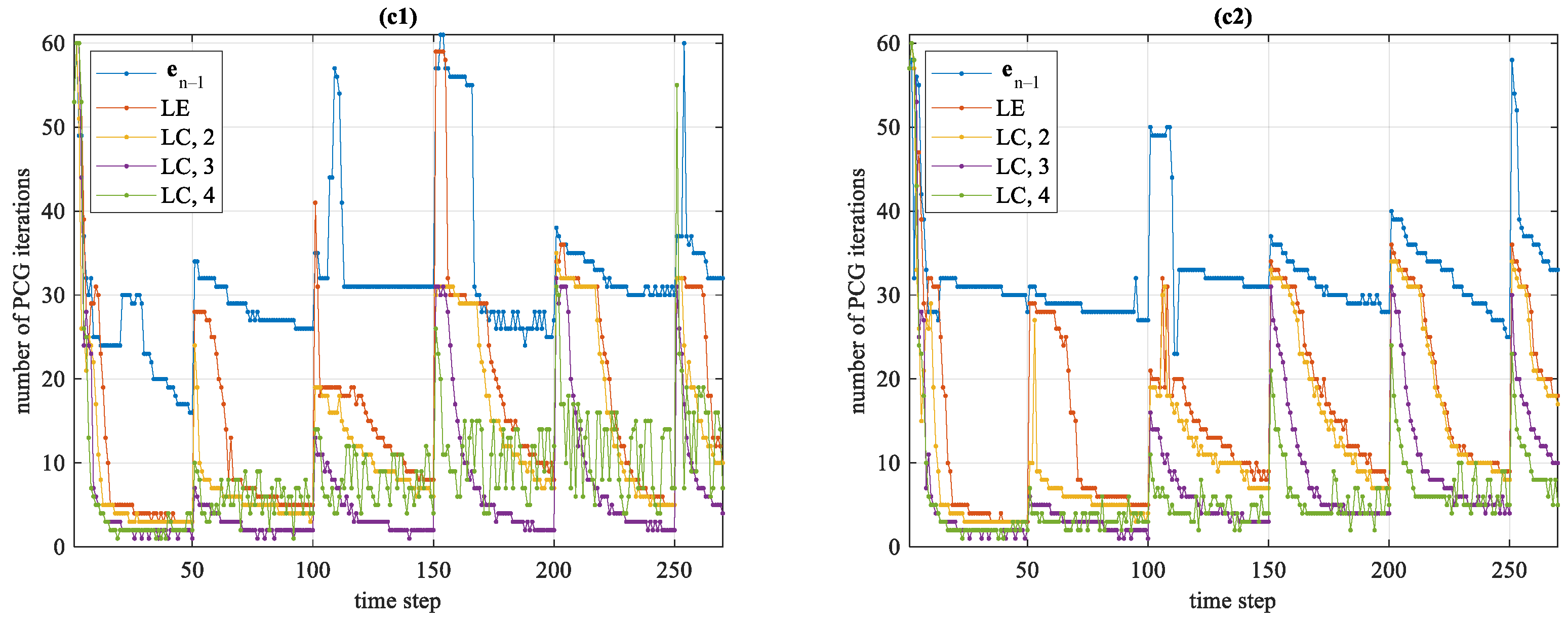
Next, we compare the efficiency of iterative solver by showing the computational time at each time step t step in Figure 5a, the total run time t total in Figure 5b, and the number of PCG iterations of each time step N iter in Figure 5c. The SG and MR grid cases are presented separately on the left and right columns in Figure 5. The time-stepping involves 270 steps in total, and Δ t has been enlarged five times. The general trend is that, once Δ t is enlarged, t step is also increased, which means using a larger Δ t requires more iterations to solve the system of equations. Subsequently, t step is gradually decreasing in the following time steps. This phenomenon can be interpreted as the drastic variations of e n being gradually attenuated as time passes and the equations becoming easier to solve. The performances of using different initial guesses ( x 0 ) to initialize the iterative solver are also shown. The standard approach ( x 0 = e n 1 ), the linearly extrapolated approach ( x 0 = 2 e n 1 e n 2 ), and the linearly combined approach ( x 0 = i = 1 N prev α i e n i ) arrive in the same modeling accuracy (the maximum relative differences between them are less than 0.005 % ). However, the latter two approaches require much less time for solving the equations. The linearly combined approach with N prev = 3 works more efficiently that requires much less N iter , and thereby significantly reduces t step and t total compared to the standard approach, e.g., t total = 613.7   s 201.8   s for the SG grid and t total = 328.6   s 84.8   s for the MR gird. For the linearly combined approach, the N prev = 4 case was expected to be superior to the N prev = 3 case because the former case involves one more previous time step and can be more flexible. However, the result is on the contrary. One can see that for t step and N iter of the N prev = 4 case, there exists many more perturbations in Figure 5. We may interpret this phenomenon as too much early time information dragging down the convergence on the new time step.
In addition, we compare the computational time of SG and MR grids using the linearly combined x 0 approach ( N prev = 3 case). The numbers of Degrees of Freedom ( D o F ) to solve the main system of equations D o F e and the divergence correction equations D o F ϕ for the SG gird are 1,025,815 and 337,014 in contrast to 506,615 and 165,014 on the MR grid (i.e., 49.39 % and 48.96 % of the SG grid).
As shown in Figure 5, the MR grid is undoubtedly more computationally efficient than the SG grid approach. The ratios of the averaged t step ( t ¯ step ) and t total between the MR and SG modelings are 0.31   s / 0.75   s and 84.8   s / 201.8   s , respectively. As a result, the MR grid requires only 42 % computational time of the SG grid.

4.2. Example 2

In the second numerical test, we consider a 3-D example. The model has a 1-D background consisting of 3-layers: ρ , Δ z = 200   Ω m , 50   m ; 100   Ω m , 90   m ; 50   Ω m , . Two conductive blocks are also embedded. A block with the resistivity of 10   Ω m is located at x 80   m , 20   m , y 30   m , 30   m , and z 20   m , 80   m . Another bigger and more conductive block ( ρ = 1   Ω m ) is placed at x 0   m , 80   m , y 40   m , 40   m , and the depth of z 100   m , 180   m . A 200   m × 200   m loop source is placed at the surface. A total of 400 measurement sites distribute inside the loop x , y 95   m , 95   m with 10   m interval and collect d b z / d t data in the time range of 5 × 10 6   s , 10 2 s . The SG grid has a resolution of 80 × 80 × 60 , where the central area is discretized with 10   m uniform cells. The model grid includes 15 air layers with the same discretization as in Example 1. MR grid is designed from the SG grid and has 5 sub-grids with the coarseness parameters: C s i , N z i ; | i = 1 , 5 = 2 , 5 ; 1 , 5 ; 0 , 19 ; 1 , 20 ; 2 , 11 . Note that the third common interface is located at the place between two background layers, and it also crosses the deeper conductive block. The MR grid discretization is shown in Figure 6.
Since the differences between the SG and MR grid modeling responses are hardly visible, only the MR grid solution is shown in Figure 7a. The anomalous responses caused by the conductive blocks are clearly visible. The 3-D solution using the Lanczos spectral decomposition method (SLDM) [24] was chosen as the reference to verify the accuracy of our solutions. The relative differences between SG and MR solutions against the SLDM solution are shown in Figure 7b,c, respectively. The maximum relative difference of the SG and MR grid solutions are 3.44 % at 5.29 × 10 5   s in Figure 7(b1) and 3.59 % at 2.55 × 10 4   s in Figure 7(c2), respectively.
The same efficiency parameters t step , t total , and N iter in Example 1 were also evaluated here (Figure 8). Similarly, the iterative solver using either the linearly extrapolated x 0 approach or the linearly combined x 0 approach results in much shorter run time than the standard x 0 approach. The linearly combined approach with N prev = 3 works best again, e.g., for the SG grid case, t total : 213.17   s versus 759.32   s , and t ¯ step : 0.79   s versus 2.81   s in contrast to the standard x 0 approach.
Benefiting from using the MR grid that involves much less D o F e = 480 , 060 and D o F ϕ = 156 , 139 in contrast to the SG grid ( D o F e = 1 , 120 , 220 and D o F ϕ = 368 , 219 ), we can solve a much smaller forward modeling problem and consequently further reduce the modeling time: t ¯ step = 0.79   s 0.4   s , t total = 213.17   s 107.67   s .

4.3. Example 3

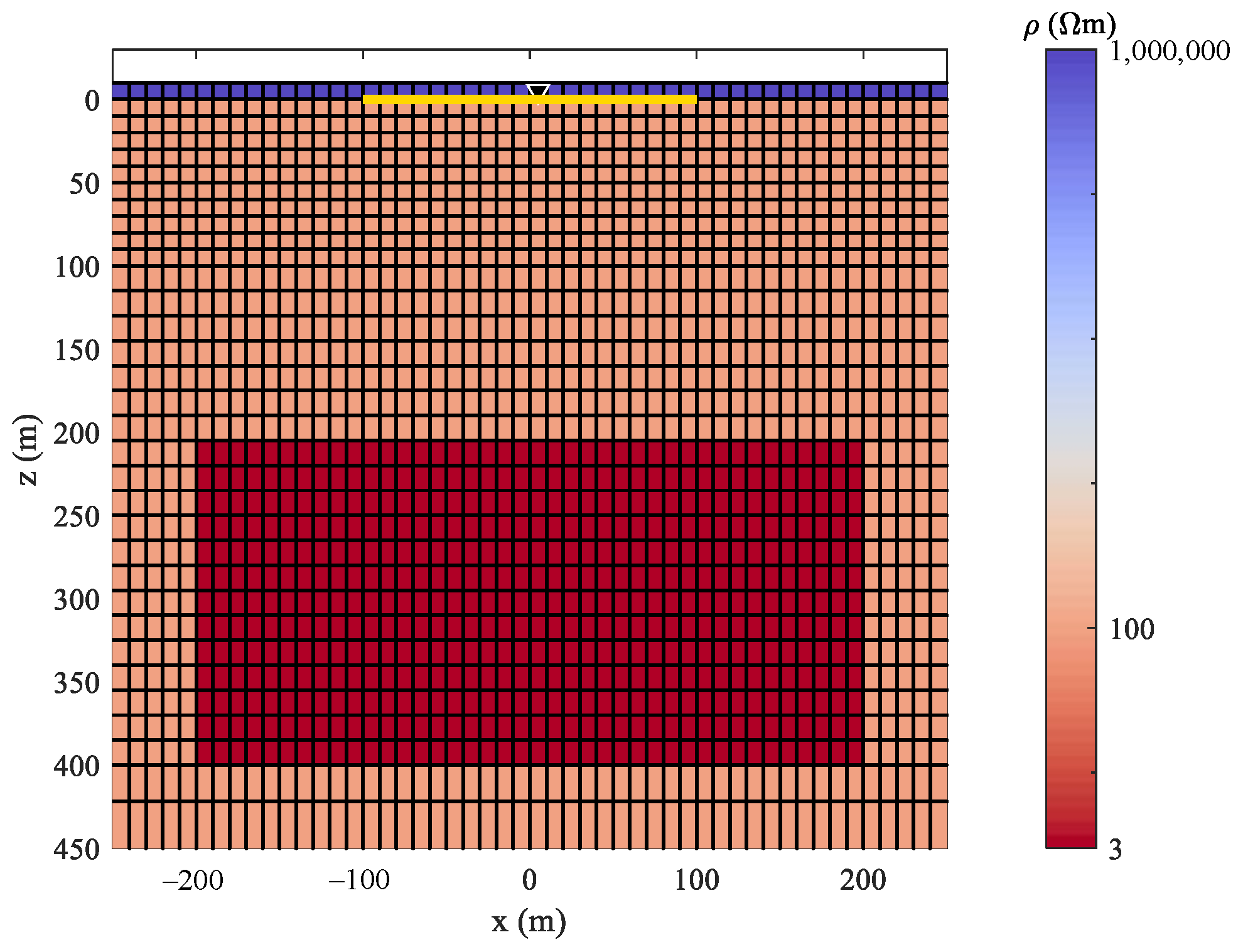
In the last example, we compare explicit and implicit schemes for different background model resistivity. Three models are tested that have a conductive block located in the same position: x , y 200   m , 200   m and z 200   m , 400   m . The resistivity of the models are different in that the anomaly block and background are 3   Ω m , 100   Ω m , 30   Ω m , 1000   Ω m , and 300   Ω m , 10 , 000 Ω m , respectively. We use the same survey design as in Example 1, i.e., 200   m × 200   m loop source and measurements of d b z / d t in 10 5 s , 10 2 s at 5   m , 5   m . For simplicity, we only compare the modeling on SG grid with the resolution of 88 × 88 × 65 . Model and grid discretization are shown in Figure 9. In previous examples, we have found that the implicit scheme modeling using the linearly combined x 0 approach with N prev = 3 has much better performance than the other initial guess approaches. Therefore, only the former approach is presented in this example.
The modeling responses are shown in Figure 10a. As expected, the amplitude of the response of the conductive model (e.g., 100   Ω m ) is generally higher than the resistive one (e.g., 10,000   Ω m ). The anomaly response in the conductive model is observed at a later time, whilst anomaly responses are visible at an earlier time for the resistive models. This phenomenon is due to the different skin depths of EM fields in those three models. The modeling responses of explicit and implicit schemes are compared, and their relative differences are shown in Figure 10b. For the models with 100   Ω m and 1000   Ω m background resistivity, the relative differences between explicit and implicit schemes are small, which are 2.34 % and 3.07 % respectively. For the 10,000   Ω m model, the relative difference is slightly higher ( 5.05 % ).
The efficiencies of the forward modeling using explicit and implicit schemes are compared and shown in Table 1. The explicit scheme usually requires more time steps ( N step ) than the implicit scheme, but each time step is faster.
It is clearly visible for the conductive ( 100   Ω m ) model that the explicit scheme took only 97.61   s to finish the job, which is more efficient than the implicit scheme ( 265.72   s ). However, the explicit scheme is strongly affected by the background resistivity. As the resistivity increases, N step is increased accordingly ( 3089 9724 30 , 296 ), and the modeling speed is degrading ( 97.61   s 1205.11   s 14 , 244.9 s ). The reason is that the EM fields propagate faster in the resistive media, and Δ t n must be suppressed to stabilize the modeling. In addition, the upward continuation boundary condition used in the explicit scheme requires the inclusion of a large area for 2-D FFT. Since FFT requires an equidistant grid that is usually discretized by the minimum horizontal edge-length to match the short wave variations of the fields, the larger area, especially at the padding cells, significantly increases the computations [5]. The same influence on t ¯ step can also be found ( 0.032   s 0.12   s 0.47   s ), which is also mainly caused by the heavier FFT computations in the resistive models. In contrast, the implicit scheme is less affected by the model’s resistivity. Even though t total is also gradually increasing for the resistive models, which means the equations took a longer time ( t ¯ step ) to be solved, the run time fluctuations are relatively stable.
Thus, the explicit scheme modeling is more efficient for the model with a conductive background, whilst the implicit scheme modeling is preferable for the resistive one.

5. Discussion

We have implemented the 3-D TEM implicit scheme forward modeling based on the second-order backward Euler method on the multi-resolution (MR) grid. The implicit scheme forward modeling requires the solution of the system of linear equations, which is often done using iterative solvers. We have found that initializing the iterative solver with a better guess has a profound influence on iterations. The standard initial guess approach usually uses the previous time step’s solution, which is too conservative. We have tested the linearly extrapolated and linearly combined approaches based on the solutions from several previous time steps to derive a better initial guess. We show that it improves the convergence rate significantly and therefore reduces the modeling time. Our result also shows the linearly combined initial guess using three previous time steps works the best. Involving more previous time steps to predict the current solution does not improve the performance further.
The implicit scheme modeling is tested using three synthetic examples against other algorithms to verify the accuracy and efficiency. The MR grid substantially decreases the number of degrees of freedom and results in better computational efficiency without compromising the accuracy.
Finally, we compare 3-D TEM forward modeling using the explicit and implicit schemes on different models and derive strategies to choose the more efficient solution. The explicit scheme generally requires more time steps than the implicit scheme, but the computational costs at each time step are lower. The result shows that the explicit scheme is more suitable for the simulation in a conductive environment, e.g., environmental studies or sedimentary basins.
In contrast, the modeling speed of the implicit scheme is less affected by the background resistivity. Hence, the implicit scheme is preferable in a resistive environment, e.g., shield areas. Future studies will implement the forward modeling into the inversion and use the real field data to examine the algorithms. We would use an initial run to verify which modeling scheme would be more efficient for certain prior model conditions. This testing can allow us to choose the modeling scheme and optimize the inversion algorithm with respect to speed and accuracy. In the previous work, we also used time-domain electromagnetic modeling to simulate electric fields at the surface for the geomagnetically induced currents simulation. Based on the results presented in this study, we expect that the implicit scheme modeling would be more suitable for this purpose.

Author Contributions

J.G.: methodology; software; writing—original draft preparation; validation; visualization. M.S. (Maxim Smirnov): conceptualization; methodology; supervision; writing—review and editing. M.S. (Maria Smirnova): methodology; writing—review and editing. G.E.: methodology; writing—review and editing. All authors have read and agreed to the published version of the manuscript.

Funding

This research was supported by the ARN project, and the project is funded by the European Union, through the Swedish Agency for Economic and Regional Growth and the Norrbotten County Council, as research project no. 20200552.

Institutional Review Board Statement

Not applicable.

Informed Consent Statement

Not applicable.

Data Availability Statement

The data presented in this study are available on request from the corresponding author.

Acknowledgments

The authors thank two reviewers for valuable comments that helped to improve the quality of the paper. We also thank Maofei Li for his help.

Conflicts of Interest

The authors declare no conflict of interest. The funders had no role in the design of the study; in the collection, analyses, or interpretation of data; in the writing of the manuscript, or in the decision to publish the results.

References

  1. Flores, C.; Peralta-Ortega, S.A. Induced polarization with in-loop transient electromagnetic soundings: A case study of mineral discrimination at El Arco porphyry copper, Mexico. J. Appl. Geophys. 2009, 68, 423–436. [Google Scholar] [CrossRef]
  2. Swidinsky, A.; Hölz, S.; Jegen, M. On mapping seafloor mineral deposits with central loop transient electromagnetics. Geophysics 2012, 77, E171–E184. [Google Scholar] [CrossRef] [Green Version]
  3. Guo, Z.; Xue, G.; Liu, J.; Wu, X. Electromagnetic methods for mineral exploration in China: A review. Ore Geol. Rev. 2020, 118, 103357. [Google Scholar] [CrossRef]
  4. Liu, Y.; Yin, C.; Qiu, C.; Hui, Z.; Zhang, B.; Ren, X.; Weng, A. 3-D Inversion of Transient EM Data with Topography Using Unstructured Tetrahedral Grids. Geophys. J. Int. 2019, 217, 301–318. [Google Scholar] [CrossRef]
  5. Börner, R.U. Numerical modelling in geo-electromagnetics: Advances and challenges. Surv. Geophys. 2010, 31, 225–245. [Google Scholar] [CrossRef]
  6. Adhidjaja, J.I.; Hohmann, G.W. A finite-difference algorithm for the transient electromagnetic response of a three-dimensional body. Geophys. J. Int. 1989, 98, 233–242. [Google Scholar] [CrossRef] [Green Version]
  7. Oristaglio, M.L.; Hohmann, G.W. Diffusion of electromagnetic fields into a two-dimensional earth: A finite-difference approach. Geophysics 1984, 49, 870–894. [Google Scholar] [CrossRef]
  8. Wang, T.; Hohmann, G.W. A Finite-difference, Time-domain Solution for Three-dimensional Electromagnetic Modeling. Geophysics 1993, 58, 797–809. [Google Scholar] [CrossRef] [Green Version]
  9. Haber, E.; Ascher, U.; Oldenburg, D.W. 3D forward modelling of time domain electromagnetic data. In SEG Technical Program Expanded Abstracts 2002; Society of Exploration Geophysicists: Tulsa, OK, USA, 2002; pp. 641–644. [Google Scholar]
  10. Um, E.S.; Harris, J.M.; Alumbaugh, D.L. 3D time-domain simulation of electromagnetic diffusion phenomena: A finite-element electric-field approach. Geophysics 2010, 75, F115–F126. [Google Scholar] [CrossRef]
  11. Oldenburg, D.W.; Haber, E.; Shekhtman, R. Three dimensional inversion of multisource time domain electromagnetic data. Geophysics 2013, 78, E47–E57. [Google Scholar] [CrossRef] [Green Version]
  12. Um, E.S.; Harris, J.M.; Alumbaugh, D.L. An iterative finite element time-domain method for simulating three-dimensional electromagnetic diffusion in earth. Geophys. J. Int. 2012, 190, 871–886. [Google Scholar] [CrossRef] [Green Version]
  13. Domnikov, P.A. Speedup of three-dimensional finite element geoelectromagnetic fields modelling in time domain. In Proceedings of the 2016 13th International Scientific-Technical Conference on Actual Problems of Electronics Instrument Engineering (APEIE), Novosibirsk, Russia, 3–6 October 2016; Volume 2, pp. 244–246. [Google Scholar]
  14. Haber, E.; Heldmann, S. An octree multigrid method for quasi-static Maxwell’s equations with highly discontinuous coefficients. J. Comput. Phys. 2007, 223, 783–796. [Google Scholar] [CrossRef]
  15. Horesh, L.; Haber, E. A second order discretization of Maxwell’s equations in the quasi-static regime on OcTree grids. SIAM J. Sci. Comput. 2011, 33, 2805–2822. [Google Scholar] [CrossRef]
  16. Cherevatova, M.; Egbert, G.; Smirnov, M.Y. A multi-resolution approach to electromagnetic modelling. Geophys. J. Int. 2018, 214, 656–671. [Google Scholar] [CrossRef]
  17. Gao, J.; Smirnov, M.; Smirnova, M.; Egbert, G. 3-D DC Resistivity Forward Modeling Using the Multi-resolution Grid. Pure Appl. Geophys. 2020, 117, 2803–2819. [Google Scholar] [CrossRef] [Green Version]
  18. Gao, J.; Smirnov, M.; Smirnova, M.; Egbert, G. 3-D time-domain electromagnetic modeling based on multi-resolution grid with application to geomagnetically induced currents. Phys. Earth Planet Inter. 2021, 312, 106651. [Google Scholar] [CrossRef]
  19. Yee, K. Numerical Solution of Initial Boundary Value Problems Involving Maxwell’s Equations in Isotropic Media. IEEE Trans. Antennas Propag. 1966, 14, 302–307. [Google Scholar] [CrossRef] [Green Version]
  20. Commer, M.; Newman, G. A Parallel Finite-difference Approach for 3D Transient Electromagnetic Modeling with Galvanic Sources. Geophysics 2004, 69, 1192–1202. [Google Scholar] [CrossRef] [Green Version]
  21. Farquharson, C.G.; Miensopust, M.P. Three-dimensional finite-element modelling of magnetotelluric data with a divergence correction. J. Appl. Geophys. 2011, 75, 699–710. [Google Scholar] [CrossRef]
  22. Smith, J.T. Conservative modeling of 3-D electromagnetic fields, Part II: Biconjugate gradient solution and an accelerator. Geophysics 1996, 61, 1319–1324. [Google Scholar] [CrossRef]
  23. Auken, E.; Christiansen, A.V.; Kirkegaard, C.; Fiandaca, G.; Schamper, C.; Behroozmand, A.A.; Binley, A.; Nielsen, E.; Effersø, F.; Christensen, N.B.; et al. An overview of a highly versatile forward and stable inverse algorithm for airborne, ground-based and borehole electromagnetic and electric data. Explor. Geophys. 2015, 46, 223–235. [Google Scholar] [CrossRef] [Green Version]
  24. Druskin, V. A spectral semi-discrete method for numerical solution of 3-D non-stationary problems in electrical prospecting. Phys. Sol. Earth 1988, 24, 641–648. [Google Scholar]
Figure 1. Sketches of the ground TEM survey configuration using the loop source and the discretization of the multi-resolution grid. Red lines represent the loop source; white points represent measurement sites; the blue region indicates the air layers.
Geosciences 11 00257 g001
Figure 2. Sketch of time-stepping using the explicit scheme in the modified version of the Du Fort-Frankel method and the implicit scheme based on the second-order backward Euler method.
Geosciences 11 00257 g002
Figure 3. Example 1: model, measurement configuration, and MR grid discretization (central region). Yellow line and black cone denote loop source and observation site, respectively. Air resistivity ( 10 6 Ω m ) is not shown with color.
Geosciences 11 00257 g003
Figure 4. Example 1: (a) forward modeling responses; (b) relative differences of the 3-D SG and MR grid solutions against the 1-D semi-analytical solution.
Geosciences 11 00257 g004
Figure 5. Example 1: efficiency comparison between SG (left column) and MR (right column) grid approaches. Abbreviations denote different initial guess ( x 0 ) approaches: (i) e n 1 , standard approach, x 0 = e n 1 ; (ii) LE, linearly extrapolated approach, x 0 = 2 e n 1 e n 2 ; (iii) LC, N prev = 2 , 3 , 4 , linearly combined approach, x 0 = i = 1 N prev α i e n i . Rows 1–3 show the time usage of each time step, the run time during time-stepping, and the number of PCG iterations of each time step, respectively.
Geosciences 11 00257 g005
Figure 6. Example 2: model, measurement configuration, and MR grid discretization (central region). Yellow line and black points denote loop source and observation sites, respectively. Discretization of air layers is the same as in Example 1 and is omitted here.
Geosciences 11 00257 g006
Figure 7. Example 2: (a) Forward modeling response ( d b z / d t ) of MR grid approach. Relative differences of SG grid solution (b) and MR grid solution (c) against the SLDM solution. Rows 1–3 correspond to the time gates at 5.29 × 10 5   s , 2.55 × 10 4   s , and 7.27 × 10 4   s , respectively.
Geosciences 11 00257 g007
Figure 8. Example 2: efficiency comparison between SG (left column) and MR (right column) grid approaches. Abbreviations denote different initial guess ( x 0 ) approaches: (i) e n 1 , standard approach, x 0 = e n 1 ; (ii) LE, linearly extrapolated approach, x 0 = 2 e n 1 e n 2 ; (iii) LC, N prev = 2 , 3 , 4 , linearly combined approach, x 0 = i = 1 N prev α i e n i . Rows 1–3 show the time usage of each time step, the run time during time-stepping, and the number of PCG iterations of each time step, respectively.
Geosciences 11 00257 g008aGeosciences 11 00257 g008b
Figure 9. Example 3: 100   Ω m model, measurement configuration, and the grid discretization (central region). Yellow line and black cone denote loop source and observation site, respectively. The explicit scheme modeling grid is shown here in which only one air layer exists; the implicit scheme modeling grid has 15 air layers like the other examples. The other two models have the same grid discretization, only the resistivity of background and anomaly block change to 30   Ω m , 1000   Ω m and 300   Ω m , 10 , 000 Ω m .
Geosciences 11 00257 g009
Figure 10. Example 3: (a) forward modeling responses; (b) relative differences between the solutions of explicit and implicit schemes.
Geosciences 11 00257 g010
Table 1. Example 3: comparison of forward modeling speeds between explicit and implicit schemes.
SchemeParameter100 Ω m Model1000 Ω m Model10,000 Ω m Model
explicit D o F D o F e = 1 , 144 , 050 , D o F h = 1 , 168 , 112
N step 30899724 30 , 296
t total 97.61   s 1205.11   s 14 , 244.9 s
t ¯ step 0.032   s 0.12   s 0.47   s
2-D FFT area ( x , y ) 2555   m , 2555   m 10 , 235 m , 10 , 235 m 20 , 475 m , 20 , 475 m
implicit D o F D o F e = 1 , 471 , 953 , D o F ϕ = 484 , 416
N step 270270270
t total 265.72   s 297.92   s 356.81   s
t ¯ step 0.98   s 1.1   s 1.32   s
Publisher’s Note: MDPI stays neutral with regard to jurisdictional claims in published maps and institutional affiliations.