Advanced Determination of Heat Flow Density on an Example of a West Russian Oil Field

Abstract

Reliable geothermal data are required for basin and petroleum system modeling. The essential shortcomings of the methods and results of previous geothermal investigations lead to a necessity to reappraise the data on the thermal properties and heat flow. A new, advanced experimental basis was used to provide reliable data on vertical variations in the thermal properties of formation and heat flow for the area surrounding a prospecting borehole drilled through an unconventional hydrocarbon reservoir of the Domanik Formation in the Orenburg region (Russia). Temperature logging was conducted 12.5 months after well drilling. The thermal properties of the rocks were measured with continuous thermal core profiling on all 1699 recovered core samples. Within non-cored intervals, the thermal conductivity of the rocks was determined from well-logging data. The influence of core aging, multiscale heterogeneity and anisotropy, in situ pressure and temperature on the thermal properties of rock was accounted for. The terrestrial heat flow was determined to be 72.6 ± 2.2 mW·m⁻²—~114% larger than the published average data for the studied area. The experiment presents the first experience of supporting basin modeling in unconventional plays with advanced experimental geothermal investigations.

1. Introduction

Information about the actual heat flow and thermal properties of rock is necessary for modeling sedimentary basins and oil and gas-bearing systems [1]. The reliability of the modeling results depends on the reliability of these data. It has been shown that uncertainties in these data lead to a severe reduction in the reliability of basin and petroleum system modeling [2] conducted on areas of the Earth’s crust with the occurrence of unconventional reservoirs, where only scarce special geothermal surveys have been conducted recently. All of this has led to the necessity to measure the thermal properties of rock and assess variations of heat flow density when drilling a prospecting and appraisal well located in the Orenburg region on the European part of Russia in the southern part of the piedmont of the western Urals.

In the 1980–2000s, in geothermal surveys in the framework of national and international scientific continental deep drilling programs, serious problems were identified in the methods and results of experimental geothermics concerning the investigation of areas with shale oil deposits. For the depths of more than 2.5–3 km, a significant systematic mismatch (by 40–130%) was identified between the previous data on heat flow density determined using data on the thermal conductivity of rocks and the temperature gradient [3] and the new results of the heat flow determination [4,5,6,7,8,9]. This revealed the necessity for a severe reappraisal of data on deep heat flow. The unreliability of previous data on deep heat flow resulted from imperfections in the previously used methods of experimental geothermal investigations. For instance, in many previous cases, the thermal conductivity of rocks was determined not via measurements on core samples from the investigating well but with the help of existing databases for similar rock types from other (often distantly located) wells. These practices were common for most wells drilled in the Urals and the piedmont of the western Urals [10]. In the case of thermal conductivity measurements on cores, usually, insufficiently representative collections of core samples have been studied. In most cases, the anisotropy and different-scale heterogeneity (at the core–sample scale and drilling interval scale) were not considered. The measurements were carried out under atmospheric thermobaric conditions without considering the effect of in situ conditions [10]. The problems of obtaining representative data on rock thermal conductivity were conditioned by the fact that the use of traditional measuring instruments requires specific procedures to eliminate the effect of contact resistance between the surface of the studied rock sample and the measuring probe [11]. The necessary polishing of rock samples with the required quality is difficult, especially in the case of sedimentary reservoir rocks. Moreover, the use of a liquid lubricant is unacceptable due to its penetration into the porous-fractured space and the ensuing changes in the properties of the samples. The application of the required pressure to porous and fractured samples during measurements can lead to their partial or complete destruction. Measuring the thermal conductivity without the water saturation of the samples is a widespread practice that has led to values of the thermal conductivity and heat flow data that were lower by 20% to 40% [12], and in case of fluid saturation, the saturation was not conducted under vacuum. The volumetric heat capacity of rock, the data on which, along with the thermal conductivity, are necessary for basin modeling and estimates of the paleoclimate effect [10,12,13], was found only in rare instances [10,11].

Another typical problem while determining the heat flow was the lack of acceptable quality data on the temperature gradient. The researchers often calculated the temperature gradient using the results of temperature logging that was conducted immediately after the completion of drilling, when the temperature and its gradient had not reached their equilibrium values. Before scientific continental deep drilling, the researchers did not practically consider the possibility of significant vertical variations of the conductive component of the heat flow at depths of more than 300–500 m, assuming its stability at deeper levels. Therefore, the average value of the conductive component of the heat flow was determined using the average temperature gradient and thermal conductivity within the investigated depth intervals [10,14,15]. Another aspect that resulted in underestimations of the heat flow was the insufficient depth of the investigating wells (up to 2000 m; in most cases, the well depth varied from 500 to 1500 m), while the temperature gradient was determined using the data on temperature on the surface and at the bottom hole. These data were averaged along the entire well or investigating interval without considering the influence of the paleoclimate and fluid migration in the upper parts of the sedimentary section.

These issues make the previous data on heat flow practically inapplicable for solving most geological and geophysical problems. Thus, it is necessary for new, correct experimental estimates of heat flow to be obtained on the basis of a novel experimental and methodological framework of geothermics [16]. Concurrently, the estimates of heat flow data should account for the paleoclimate effect. In particular, it is necessary to enhance the quality of basin models that include the unconventional petroleum resources of Russia (they are the Domanik Formation, located in the Volga–Ural and Timanv–Pechora oil and gas region, the Bazhenov Formation, located in the West Siberian oil and gas basin, etc. [17,18,19,20,21,22]).

The reasons mentioned above have conditioned extensive experimental geothermal studies of the prospecting and appraisal well located in the zone of the junction of the East Orenburg arched uplift with the northern part of the Buzulukskaya valley, in the area of the Balekinsky licensed block of Gazpromneft Orenburg LLC (Orenburg region) to maintain basin and petroleum system modeling by providing reliable geothermal source data. Accounting for the scope of the work, the complex character of investigations, the application of the novel experimental and methodological framework of the geothermics, and the joint efforts of scientific and industrial organizations, it is fair to assume that this study was performed for the first in the field of global petroleum geophysics. Moreover, the deposits of the Domanik type are highly differentiated both along the geological profile and laterally [23]. Because of that, the obtained results for the investigating well are of a particular value. The obtained experimental data on thermal properties and heat flow were further used to develop a basin model for the studied area of the field. The first simulation results [24] show that the new data redefine the transformation ratio of organic matter and therefore the generated petroleum mass (by ~27%).

2. Materials and Methods

2.1. Object of Study

The studied well belongs to the group of wells drilled in the framework of the development of the unconventional Domanik resources in the Volga–Urals region [18,21,22,23]. The well was drilled on the territory of the Baleikinskoye field that had been discovered in 2006 in the Orenburg region of the Russian Federation (Figure 1). Drilling was started on 6 December 2013 and finished on 22 April 2014. The drilling depth was 3827 m. The construction of the well was finalized with the descent of the production string and cementing of the borehole annulus to the depth of 3827 m. The well is almost vertical.

Figure 1. Geographic location of the understudy well on the heat flow map [25]. The large red point indicates the well’s location.

Figure 1. Geographic location of the understudy well on the heat flow map [25]. The large red point indicates the well’s location.

The borehole was drilled through the Quaternary, Paleozoic, and Upper Proterozoic sediments (

Table 1. Characteristics of the sediments from the investigated well based on the analysis of the recovered cores.

№	Rock Type	Age	Logging Depth, m	N *
1	In the upper part, anhydrite–dolomite rock, in the middle and lower parts, limestone	P1ar	1348.50–1366.10	135
2	Bioclastic limestones with rare inclusions of anhydrite and porous intervals	C1t	2612.29–2629.20	145
			2657.00–2665.74	73
3	Bioclastic limestones that have (1) rare dolomitized intervals and are (2) porous, (3) cavernous, (4) oil-saturated in some intervals, (5) with a rare interbedding of argillites.	D3zv	2737.30–2746.02	78
			2754.90–2763.60	65
			2794.90–2812.50	143
4	Bioclastic limestones that are porous, fractured, with rare interbedding of argillites.	D3fm	2916.90–2934.34	143
6	In the upper part, quartz sandstones and argillites; in the middle part, limestones and argillites; and in the lower part, marlstones.	D3p–D2ml	3506.40–3539.30	272
7	Interbedding of quartz sandstones and shaly siltstone.	D2ar	3585.38–3597.40	92
8	Bioclastic limestones with oil saturated intervals and thin layers of sandstones.	D2vb–D2af	3619.20–3630.68	89
9	Bioclastic limestones that are unevenly oil-saturated.	D2af	3650.00–3667.08	93
10	In the upper part, organogenic limestone; in the middle and lower parts, quartz sandstones and argillites.	D2bs–D1kv	3756.70–3776.31	148
11	Argillites, sandstones and gravelites.	V–R	3782.64–3812.12	223

* N—number of core samples.

). The Quaternary sediments are represented by clays, argillaceous sand grounds, and conglomerates. The Paleozoic group is represented by the deposits of Permian, Carbonous, and Devonian systems, and the Upper Proterozoic group is represented by the Vendian–Riphean formations. The Upper-Middle Perm sedimentary rocks are characterized by alternating shales, siltstone, and sandstones with subordinate interlayers of carbonate rocks. The Lower Permian and Carboniferous formations are represented by carbonate rocks (unevenly sulfated dolomite and limestone). There is a powerful sulfate–halogen formation in the upper part of the Lower Permian sediments (743.0–1192.0 m), which forms a regional seal. Limestones prevail in the Upper-Middle Devonian series. Sandstones and gravelstone represent the Lower Devonian series of the Paleozoic group and the Upper Proterozoic sediments.

In the depth interval of 3371.9 to 3452.0 m, the borehole crossed the Domanik Formation.

The core sample lengths ranged from 31 to 404 mm with an average length of 99 mm (Figure 2).

2.2. Workflow

The implementation of the novel experimental basis of thermal petrophysics provided a qualitatively new framework for determining heat flow density. The workflow for heat flow determination is plotted in Figure 3 and includes the following steps:

• Temperature logging in the suspended well is conducted (Section 2.3). Concurrently, the continuous thermal core logging for all available full-sized cores is conducted (Section 2.4.1).
• The continuous thermal core logging of all recovered full-size core samples is conducted at atmospheric pressure and temperature (see Section 2.4.1).
• Based on the results of thermal core logging and the analysis of lithological and stratigraphic data, the reasonable selection of core plugs (see Section 2.4.2) for subsequent measurements of thermal properties at full saturation and elevated pressure and temperature is conducted.
• The investigations of rock thermal properties at elevated temperatures and pressures (Section 2.4.3) and at different saturations are conducted (Section 2.4.2). Based on the obtained results, the nature of thermal anisotropy (textural or technogenic micro-anisotropy) is determined.
• The rock thermal properties are determined within not-cored intervals from well-logging data based on a novel technique (Section 2.5, [26]) accounting for the estimated rock anisotropy.
• The equivalent thermal conductivity is calculated for intervals with experimental and predicted (from well-logging) data on thermal conductivity at atmospheric temperature and pressure (Section 2.6). Concurrently, the temperature gradient is calculated for the intervals with data on rock thermal properties (Section 2.3).
• Based on the results of the measurements of the thermal properties of core plugs from a reasonably selected collection, the corrections for in situ saturation, temperature, and pressure are applied for equivalent thermal conductivities accounting for multiscale rock heterogeneity, the effects of core changes during storage, and textural and micro-anisotropy factors.
• The calculation of heat flow density is performed for intervals with data on rock thermal properties and temperature gradients. The separate method of heat flow determination (when the upper and lower estimates of interval thermal conductivity are used; see Section 2.6) was applied. The calculation of the conductive component of the heat flow density is carried out according to the Fourier equation for the stationary conductive heat transfer [3]:

$$\overrightarrow{q}=-{\lambda }_{equiv}·gradT$$

(1)

where q is the heat flow density vector, gradT is the temperature gradient, and λ_equiv is the so-called equivalent thermal conductivity. In the general case, λ_equiv is the thermal conductivity of the heterogeneous medium for the depth interval, where the thermal gradient is averaged. In case the heat flow is estimated to be below or above the investigated depth intervals, the influence of radiogenic heat, paleoclimate and advective component should be assessed. The vertical variations of heat flow are negligibly affected by the radiogenic heat, which should increase the heat flow in the upper parts of the geological profile. According to [1], the effect of radiogenic heat in most cases amounts to less than 1.5%.

Additionally, we assessed the effect of the paleoclimate on the temperature gradient using the obtained experimental data on rock thermal properties via mathematical modeling. The estimation of the possible effect of the advection is beyond the scope of the paper and requires special efforts and information on the formation and mass transfer processes in the area under study.

2.3. Temperature Logging

Temperature logging was conducted in December 2017. Before the temperature logging, the well was suspended for 12.5 months. At the time of temperature logging, the well bottom was at 3610 m. The depth interval from 0 to 3610 m was available for continuous temperature logging during the descent and lifting of the logging tool. The sampling interval of the temperature measurements was 0.1 m. The cement plug at 3610 m prevented logging measurements below this depth.

The level of random temperature fluctuations in the measurement process did not exceed 0.03 °C. The temperature resolution was 0.005 °C, and the thermal inertia did not exceed 4.0 s, according to the laboratory testing results.

The main temperature measurements were conducted while descending the measuring tool at a rate of 600 m·h⁻¹. Additional temperature measurements were conducted while lifting the measuring tool with the same rate.

According to the results of our long-term geothermal investigations, the time required for the temperature gradient to reach its equilibrium after the completion of drilling was not more than 4 to 5 weeks for the lower depth intervals, comprising up to 25–30% of the total length of the borehole (at 3000 to 5500 m deep) [27]. Since more than 3.5 years have passed since the completion of the well and more than 12.5 months have passed since the last operation, the temperature field in the well and the surrounding space can be considered as being at equilibrium for the depth interval from 1300 to 3550 m.

Three logging measurements were conducted in total to control the stability of the temperature field, with a time interval of 24 h. Each time, the temperature was registered during descending and lifting of the measuring tool. The first time, the temperature was registered along the entire well from the wellhead to the bottom of 3610 m, both during the descent and lifting of the measuring tool. At two subsequent measurements, the temperature was registered (with a speed of up to 600 m·h⁻¹) to control the quality of measurements in the depth interval of 2400 to 3610 m both while descending and lifting the measuring tool. As revealed from the comparison of three temperature measurements made at a 24 h interval, the absolute difference did not exceed the temperature resolution. Consequently, the temperature gradients calculated for the downward and upward runs were perfectly reproducible.

2.4. Methods for Measuring Thermal Properties of Rocks

The determination of the thermal properties of the rock included the following set of studies:

• The continuous profiling of thermal properties with an optical scanning technique of all recovered full-sized cores (cores were sawed in half along their axis) from the studied well. During scanning, the parallel and perpendicular components of thermal conductivity were determined, and the assessment of the textural anisotropy and microanisotropy of rocks [10] was performed.
• Determining the effect of the core change on rock thermal conductivity after the extraction of cores from the packing containers via additional measurements on a representative collection of standard core samples with subsequent corrections of the results of thermal core logging.
• Measurements of thermal properties at elevated temperatures on standard core plugs with a combination of measurements with the optical scanning laser setup [26], DTC-300 device (TA instruments), and DSC 214 Polyma (NETZSCH).
• Determining the dependencies of thermal properties on the porosity and type of pore fluid via the measurement of thermal conductivity components for parallel and perpendicular directions to the bedding plane and volumetric heat capacity at different saturations (sequentially dried, saturated with synthetic brine and oil under vacuum conditions) on the collection of standard core plugs using a laser setup for optical scanning.
• Measuring thermal conductivity and volumetric heat capacity on core cuttings at atmospheric and in situ temperatures [26].
• Determining rock thermal properties from well-logging data within intervals that were not cored [28].

Representative collections of core samples for additional studies were selected using the results of the continuous thermal core logging of full-sized cores and their lithological description.

Using the results of the complex studies of thermal conductivity and the results of the assessment of the degree of textural anisotropy and microanisotropy of rocks (caused by the oriented micro-cracks, etc.), a calculation of the vertical equivalent thermal conductivity was performed for different depth intervals along the borehole accounting for the in situ conditions. These depth intervals were selected in correspondence with the results of determining the equilibrium temperature gradient and the analysis of the nature of vertical variations in the temperature gradient and rock thermal conductivity. After that, the conductive component of the heat flow density for each selected depth interval and the terrestrial heat flow was determined by multiplying the vertical equivalent thermal conductivity and the equilibrium temperature gradient.

2.4.1. Continuous Thermal Core Logging

Measurements of the thermal properties of rocks from full-sized cores were conducted using a field lamp device for optical scanning [11]. During non-contact scanning, the thermal property profiles were registered, and after completing the scanning for each core sample, the following information was immediately yielded:

• continuous profiles of thermal conductivity, thermal diffusivity, and volumetric heat capacity with a spatial resolution of about 1 mm;
• values of thermal conductivity and thermal diffusivity for parallel and perpendicular directions to the bedding plane and the associated thermal anisotropy coefficient, as well as the rock the volumetric heat capacity;
• the thermal heterogeneity factor of the sample (β), which was as follows:

β = (λ_max − λ_min) λ_avg⁻¹

(2)

where λ_min and λ_max are the minimum and maximum thermal conductivity values within the thermal conductivity profile for each core sample, and λ_avg is the average value of thermal conductivity within the profile for each core sample. The theoretical background of the optical scanning technique is comprehensively described in [11].

The determination of the thermal conductivity components for parallel and perpendicular directions to the bedding plane was performed via a combination of measurements along two mutually perpendicular directions for each core sample [11]. When scanning along the vertical axis of the full-sized core, the profile of the thermal conductivity component for parallel direction to the bedding plane was registered. The thermal conductivity component for perpendicular direction to the bedding plane was determined when scanning along the perpendicular direction to the vertical axis of the full-sized core. The scanning speed was 5 mm·s⁻¹. The total relative measurement uncertainty did not exceed ±2.5% for the thermal conductivity (with a measurement precision not exceeding 1.5%), ±4% for the thermal diffusivity, and ±5% for the volumetric heat capacity (measurement uncertainties are reported for 0.95 confidence level).

For each of the 1699 full-sized core samples recovered from the well during drilling, a series of measurements of the thermal properties were conducted in the core storage via the continuous thermal core logging with the combination of scanning for two mutually perpendicular directions [29]. The measurements were performed on a flat surface of core samples, sawed along their vertical axis (the volumetric ratio of the sawed parts was 1:2). The core samples were stored under atmospheric conditions for about a year after being recovered from the borehole.

2.4.2. Measuring Thermal Properties of Rock on Core Plugs

The core samples dried out during storage, resulting in a considerable decrease in the thermal properties of rock. Previously, the effects of fluid saturation on thermal properties were in most cases neglected during the calculation of the heat flow density [12]. Our practice of thermophysical rock investigation included, as a mandatory step, special investigations of water-saturated core plugs from a representative sample collection. That collection was reasonably selected via the analysis of the results of thermal core logging, well-logging data, and the results of petrophysical laboratory investigations. The measurements of the thermal properties and the porosity of these samples allowed us to establish the dependency of the degree of change of thermal properties at full water saturation (compared to the continuous thermal profiling data on the full-sized cores) from rock porosity. This allowed us to correct the results of continuous thermal core logging for in situ saturation using data on rock porosity in the corresponding depth intervals. Data on rock porosity could be inferred both from results of laboratory investigations of standard core plugs and from well logging data.

Based on the results of the thermal core logging of full-sized cores and the identification of typical lithotypes for corresponding depth intervals, 19 core plugs were reasonably selected to measure thermal properties at different saturations and to measure rock thermal conductivity at elevated in situ temperatures. The reasonable selection of standard core plugs was carried out according to the following procedure. For each typical lithotype from the corresponding depth interval, the distribution histograms for the thermophysical properties of rocks were calculated using the results of continuous thermal core logging. Using these histograms, the most common values of the corresponding property were identified (one for unimodal and several for multimodal distributions). Then, using data on the scanning line length (recorded automatically during thermal core logging), the depth intervals containing at least 100 mm long full-sized cores were selected. This was necessary to core standard cylindrical core plugs with dimensions of 50 × 20 mm. After that, using the results of the continuous thermal core logging, the average value of the thermal conductivity for a parallel direction to the bedding plane, the average value of the volumetric heat capacity of rock, and the thermal heterogeneity factor were determined for the selected intervals (that were at least 100 mm long). For each typical lithotype from corresponding depth intervals, the depth intervals were marked, in which the average values of the thermal properties were as close as possible to the typical values for the lithotype (according to the calculated distribution histograms). If there were more depth intervals than necessary, based on the analysis of the thermal heterogeneity factor, the most homogeneous sections were selected. After coring, additional measurements of the plug’s thermal properties were conducted with the optical scanning technique. After that, the obtained thermal properties were compared with the average values of the properties obtained from the continuous thermal core logging of full-sized cores. In case of significant divergence in the thermal conductivity and volumetric heat capacity values obtained by thermal core logging of the full-sized cores and standard core plugs (which was possible due to the destruction of the sample structure during coring or due to their increased heterogeneity), the plug was considered as inappropriate and was not used for further measurements.

From the 19 selected cores, 19 plugs were drilled out with a diameter of 50 mm and a height of 20 mm, which were intended for water saturation and subsequent measurements of the thermal properties at atmospheric conditions and at in situ temperatures. The thermal properties were measured on these samples in an “as-received” state, after extraction and drying, and after saturating with the synthetic brine under vacuum. During fluid saturation, an aqueous solution was used with a mineralization of 250 g·L⁻¹, corresponding to the average value of mineralization of reservoir water from the investigated well section.

The thermal properties of standard core plugs were measured at atmospheric conditions with a new optical scanning instrument that includes a continuously operating semiconductor laser as a heat source. The new instrument enables measurements of rock samples with a length, width, and thickness of 10 mm and greater with an increased spatial resolution (from 0.2 mm) and a changeable depth of investigation. The metrological characteristics of the device (measurement errors) are the same as reported for the lamp version of the optical scanning instrument. Optical scanning was performed in two mutually perpendicular directions (for parallel and perpendicular directions to the bedding plane) on each flat surface of the cylinders [11]. As a result, for each standard core plug and for each state (“as received”, dry, and water-saturated), components of thermal conductivity for parallel and perpendicular directions to the bedding plane were measured, as well as the thermal anisotropy coefficient, the volumetric heat capacity, and the thermal heterogeneity factor.

2.4.3. Determining Corrections for Thermal Conductivity at In-Situ Temperature and Pressure

The thermal conductivity measurements at elevated temperatures were conducted on 10 core samples that were saturated with a mineralized water solution and had a cylindrical form with a diameter of 50 mm and a height of 20 mm. The measurements were conducted with the DTC-300 setup (TA Instruments) at an elevated temperature that corresponded to the temperature of core depth.

The corrections for the effect of in situ pressure on rock thermal conductivity were inferred from literature data [30,31] accounting for lithology and in situ pressure.

2.5. Well-Log Based Determination of Rock Thermal Conductivity

In this research, we applied a recently developed, novel method for determining the thermal conductivity and volumetric heat capacity of rock within not-cored intervals from well-logging data [28]. This method allows the determination of principal components of the thermal conductivity and the volumetric heat capacity of the rock. The novel method is based on the application of continuous thermal core logging, advanced thermal conductivity models, and machine learning algorithms. The method allows accounting for in situ temperature and pressure, rock heterogeneity, and thermal anisotropy.

A detailed workflow of the developed method is given in [28]. The new method for the well-log based determination of thermal conductivity and volumetric heat capacity consists of five main steps:

• The geological and geophysical data from the investigated well are analyzed. In addition, vertical variations of temperature and pressure in the investigating geological profile are analyzed to account for the effect of in situ thermobaric conditions on the thermal properties of rock.
• The directions of the principal axes of thermal conductivity tensors of rock are determined. The directions can be determined via a set of experimental investigations of representative core samples [11] or via well-logging data. After that, a continuous thermal core logging of all recovered core samples is conducted. Thermal core logging is conducted along the established directions of principal axes of the thermal conductivity tensors of the rock. Simultaneously, the reservoir saturation in the reference and target intervals of the investigating wells are inferred from well-logging data.
• A regression analysis of well-logging data and data on the thermal properties of rock is performed, accounting for thermal anisotropy and saturation type. Additionally, the quality of the predictions that can be provided using the established regression model is analyzed via the comparison of the predicted and measured values of thermal properties.
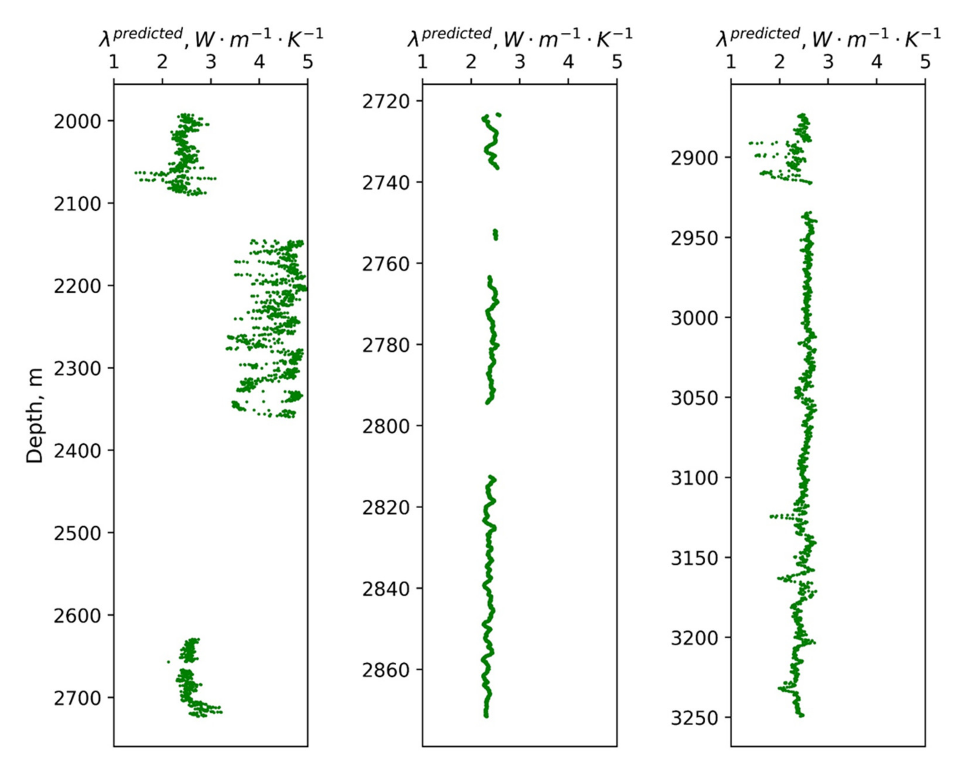
• The rock thermal properties are determined in the target interval using the results of the regression analysis (performed in the third step) from well-logging data.
• The dependencies of thermal properties on temperature and pressure are established to account for in situ conditions. These dependencies can be determined both experimentally [32,33,34] and from the available databases.

The developed method for the well-log-based determination of the thermal properties of rock includes the possibility to apply the advanced theoretical modeling of thermal conductivity and volumetric heat capacity; e.g., the application of the effective medium theory [35]. The testing of the developed method for oil shale deposits [28] and heavy oil field rocks [36] revealed that the prediction uncertainty for thermal conductivity (accounting for thermal anisotropy) and volumetric heat capacity did not exceed 10% and 6%, respectively (at the confidence level of 0.95).

2.6. Calculating Equivalent Thermal Conductivity

To calculate the heat flow density for a vertical well, the equivalent thermal conductivity for the vertical direction is required. The vertical equivalent thermal conductivity depends on macro-anisotropy (textural) and micro-anisotropy (Figure 4). Macro-anisotropy is conditioned by a layered rock texture. Micro-anisotropy can be conditioned by oriented cracks (technogenic or natural) or mineral crystals and flakes that can be anisotropic themselves.

Since the well was almost vertically drilled and stratigraphic interfaces are considered horizontal, the principal axes of thermal conductivity were oriented parallel and perpendicular to the well axis, and the temperature gradient was oriented parallel to the well axis. This made the determination of the heat flow density less complicated. In this case, the equivalent thermal conductivity (λ_equiv) could be determined as the vertical component of the rock’s thermal conductivity tensor as vectors of the heat flow density and the temperature gradient are parallel.

If micro-anisotropy is due to natural factors (oriented anisotropic grains of minerals, or oriented natural microcracks) and has to be considered jointly with macro-anisotropy (textural or transversal anisotropy) of rocks, the following equation can be used to determine the equivalent thermal conductivity [3] (necessary for calculating the heat flow density):

$${\lambda }_{equiv.L}=N·{\left({\displaystyle \sum }_{i=1}^N{\lambda }_{i\perp }{}^{-1}\right)}^{-1}$$

(3)

where λ_L is the lower estimate of the equivalent thermal conductivity, N is the number of core samples in considering depth interval, and λ_i⊥ is the thermal conductivity component perpendicular to the bedding plane for the i-th core sample accounting for thermal micro-anisotropy coefficient that was registered during thermal core logging of full-sized cores.

In the presence of a technogenically induced micro-anisotropy (due to possible microcracks along the parallel direction to the bedding plane) and in the absence of a natural micro-anisotropy, the equivalent thermal conductivity should be determined excluding the effect of rocks’ technogenic anisotropy and accounting only for macro-anisotropy (textural anisotropy). In this case, it is implied that the thermal conductivity parallel to the bedding plane (λ_‖) for each core sample characterizes the thermal conductivity of undisturbed rocks. Therefore, the equivalent thermal conductivity for the heat flow calculation shall only account for rocks’ macro-anisotropy and can be determined as follows:

$${\lambda }_{equiv.U}=N·{\left({\displaystyle \sum }_{i=1}^N{\lambda }_{i\Vert }{}^{-1}\right)}^{-1}$$

(4)

where λ_U is the upper estimate of equivalent thermal conductivity, and λ_i‖ is the thermal conductivity component for a parallel direction to the bedding plane for the i-th core sample.

3. Results

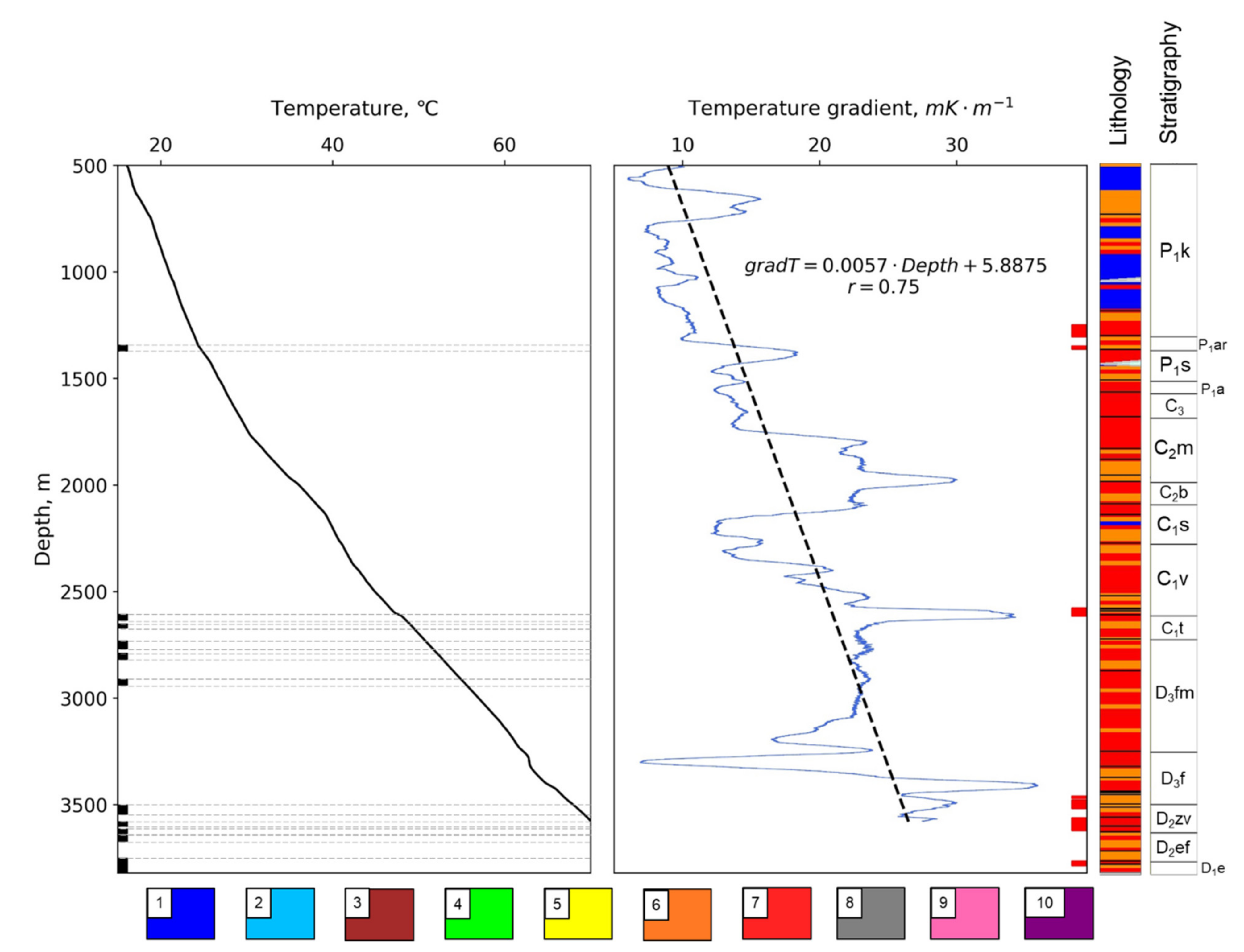
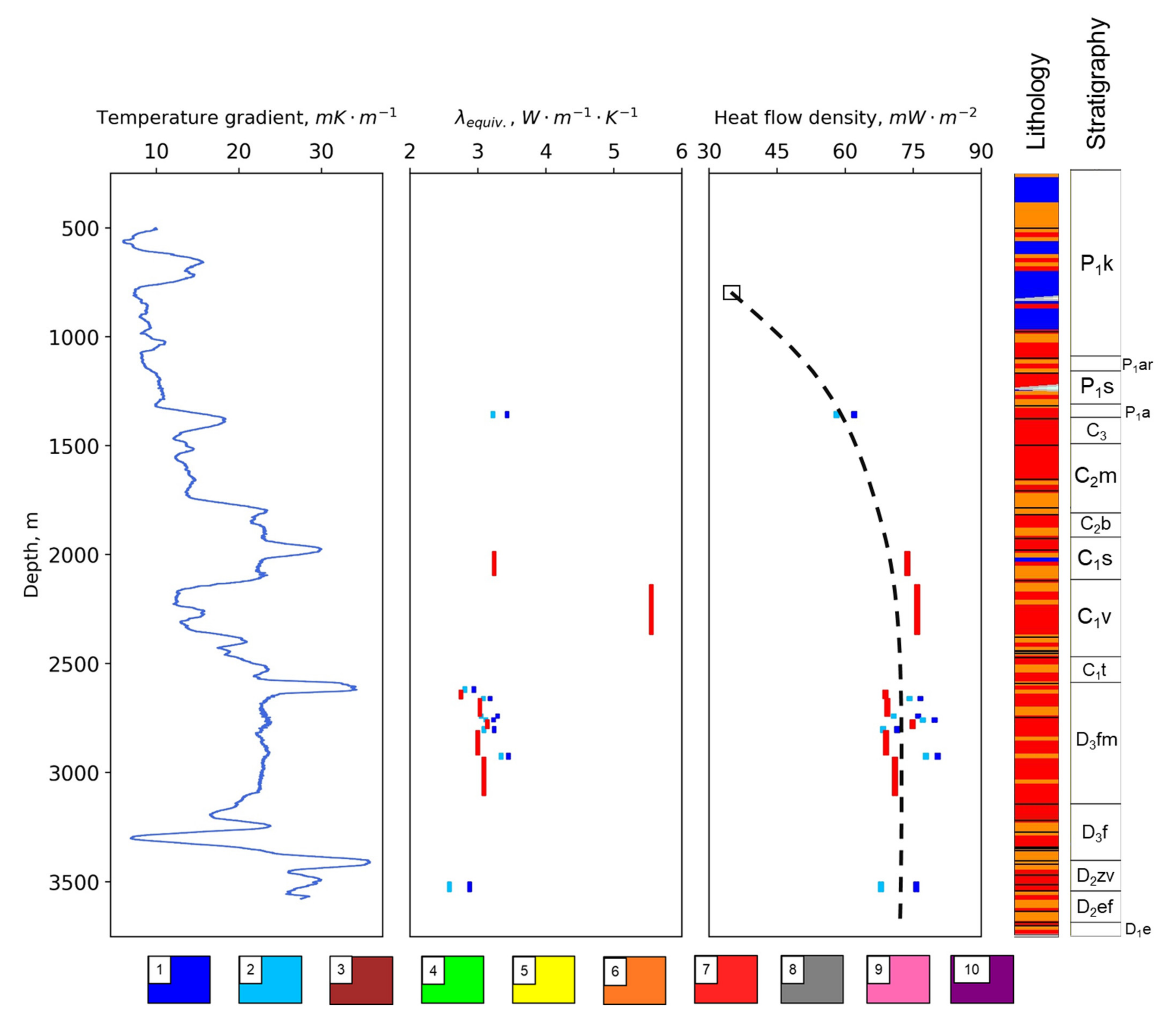
3.1. Results of Temperature Logging and Gradient Determination

The results of the temperature logging are given in Figure 5. The results of the temperature logging merge into one curve for three different measurements. For the general characterization of vertical variations of the temperature gradient, Figure 5 (right panel) plots the results of the temperature gradient calculations for each 50 m depth interval with a 10 cm step. There are local temperature anomalies in Figure 5, with a sharp change in the temperature gradient. For instance, there is a significant increase in the temperature gradient in the depth interval of 2580 to 2612 m, which is composed of loose clayous deposits of low density (less than 1.5 g·cm⁻³) and with cavernous borehole walls (caverns with a diameter of up to 0.8 m) that were formed during the drilling process. These lithology peculiarities of the horizon cause a high-temperature gradient due to the expected low effective thermal conductivity of these deposits. The local temperature anomalies in the depth interval of 3280 to 3320 m are associated with a deep technogenic perturbation of the temperature of rocks during drilling due to intensive drilling fluid loss, with a flow rate of up to 20 m³·h⁻¹ and the total loss of circulation. The depth intervals of 2580 to 2612 m and 3280 to 3320 m are not suitable for estimating the equilibrium temperature gradient of rock and are not used when evaluating the heat flow.

Previously, when numerous measurements of rock thermal properties were not accessible, researchers averaged the temperature gradient within the whole well or in a few parts. A new geothermal methodology with the continuous determination of the thermal properties of rock requires enhanced approaches for processing temperature gradient data. We applied the following approaches: (1) the determination of the temperature gradient using temperature data at the ends of the core sampling intervals; (2) the calculation of the temperature gradient in a 5 m moving window with a 10 cm step, averaging the calculation results for each core sampling interval; (3) the calculation of the temperature gradient in a 10 m moving window with a 1 cm step, averaging the calculation results for each core sampling interval; and (4) determining the temperature gradient for each core sampling interval via the least-squares method using the linear dependence between temperature and depth. The results of the temperature gradient determination via each of the described approaches are presented in

Table 2. Results of determining temperature gradient within the investigating intervals.

№	Interval, m	Temperature Gradient (Via Different Approaches), mK·m−1					Standard Deviation of Temperature Gradient, mK·m−1	Uncertainty in Estimates of Temperature Gradient		Difference between the Average Temperature Gradient and Temperature Gradient Determined within 5 m Sliding Window, %
		By Points	10 m	5 m	Corr *	Average		Absolute, mK·m−1	Relative, %
Within core sampling intervals
1	1348.50– 1366.10	18.07	17.97	17.99	18.44	18.12	0.219	0.350	1.93	−0.704
2	2612.29–2629.20	27.87	29.40	28.30	27.02	28.15	0.990	1.579	5.61	0.526
3	2657.00–2665.74	24.25	23.67	23.83	23.29	23.76	0.397	0.634	2.67	0.293
4	2737.30–2746.02	22.72	22.76	22.78	23.08	22.84	0.165	0.264	1.15	−0.242
5	2754.90–2763.60	25.57	23.65	24.53	23.74	24.37	0.891	1.421	5.83	0.638
6	2794.90–2812.50	21.99	22.01	21.83	21.49	21.83	0.241	0.384	1.76	0.000
7	2916.90–2934.34	23.22	23.29	23.21	23.31	23.26	0.050	0.080	0.34	−0.207
8	3506.40–3539.30	27.17	27.37	27.24	27.18	27.24	0.092	0.147	0.54	0.000
Within depth intervals with well-log based determinations of rock thermal properties
9	1991.00– 2091.00	22.95	23.00	22.96	22.67	22.90	0.152	0.242	1.06	0.285
10	2144.00– 2361.00	13.50	13.53	13.51	13.72	13.57	0.104	0.166	1.22	−0.402
11	2628.00– 2658.00	25.10	24.40	24.63	24.37	24.63	0.337	0.538	2.18	0.020
12	2666.00– 2737.00	22.72	22.76	22.76	22.73	22.74	0.021	0.033	0.14	0.077
13	2763.80– 2793.70	24.15	23.71	23.62	23.37	23.71	0.325	0.519	2.19	−0.388
14	2813.00– 2915.00	22.96	22.98	22.98	22.93	22.96	0.024	0.038	0.16	0.076
15	2934.90– 3100.00	22.75	22.73	22.75	22.72	22.74	0.015	0.024	0.11	0.055
	Mean						0.140	0.22	1.01	−0.04

* Linear correlation.

. Table 2 also includes the average values and standard deviations for estimates of the temperature gradients using four approaches: the absolute and relative uncertainty of estimating the average gradient, and the difference between the average temperature gradient and the results of the temperature gradient estimates when determined in the 5 m moving window. As can be seen from Table 2, the average difference between the average temperature gradient and the results of the gradient estimates determined in the 5 m sliding window was only 0.04%—i.e., it was negligible—while the difference between the average gradient estimate and the results of estimates in a 5 m sliding window was significantly less than 1%. Calculating the average temperature gradient allowed us to obtain more reliable estimates of the temperature gradient and decreasing uncertainty in temperature gradient data.

3.2. The Results of the Continuous Profiling of the Thermal Properties

The continuous profiling of thermal properties was performed on 1699 full-sized samples with a total length of 235 m from 13 depth intervals (within the range of 1348.50 to 3812.1 m) of the investigating well. Figure 6 plots an example of the distributions of the average rock thermal conductivity components for parallel and perpendicular directions to the bedding plane, the rock volumetric heat capacity, the thermal anisotropy coefficient, and heterogeneity factor for the three depth intervals. Colored dots represent core scale (Figure 6) data, whereas the grey dots represent 1 mm resolution profiles of thermal properties. The statistical characteristics of the rock thermal properties—rock thermal conductivity components for parallel and perpendicular directions to the bedding plane (λ_‖ and λ_⊥, respectively), rock volumetric heat capacity (C), the thermal heterogeneity factor for parallel and perpendicular directions to the bedding (β_‖ and β_⊥, respectively), and the thermal anisotropy coefficient K (K = λ_‖·λ_⊥⁻¹)—for each stratigraphic unit (stage, formation) are given in

Table 3. Statistical characteristics of the deposits penetrated by the well.

№	Age	Thermal Conductivity, W·m−1·K−1		KT	Thermal Heterogeneity Factor		C, MJ·m−3·K−1	N	<ϕ>, %
		λ‖aver	λ⊥aver		β‖	β⊥
1	P1ar	2.52 (0.74) (1) 1.74–5.47 (2)	2.38 (0.73) 1.41–5.15	1.07 (0.18) 1.00–2.66	0.20 (0.13) 0.04–0.90	0.16 (0.11) 0.06–0.85	2.17 (0.16) 1.84–2.80	135	10.9
2	C1t	2.15 (0.37) 1.62–5.54	2.07 (0.39) 1.04–5.54	1.04 (0.09) 1.00–1.78	0.21 (0.16) 0.06–1.32	0.16 (0.09) 0.06–0.85	2.09 (0.14) 1.72–2.62	145	9.2
		2.33 (0.26) 1.81–3.03	2.25 (0.25) 1.81–2.82	1.03 (0.06) 1.00–1.21	0.22 (0.10) 0.05–0.52	0.21 (0.10) 0.06–0.53	2.16 (0.17) 1.83–2.69	73	8.5
3	D3zv	2.54 (0.29) 1.94–3.60	2.38 (0.33) 1.32–3.49	1.08 (0.18) 1.00–2.30	0.22 (0.08) 0.08–0.49	0.18 (0.09) 0.06–0.65	2.25 (0.17) 1.92–2.94	78	4.4
		2.44 (0.14) 2.15–2.67	2.36 (0.18) 2.00–2.67	1.03 (0.05) 1.00–1.17	0.19 (0.06) 0.07–0.37	0.18 (0.11) 0.07–0.75	2.26 (0.12) 1.97–2.61	65	4.8
		2.43 (0.18) 2.07–3.18	2.34 (0.23) 1.46–3.18	1.04 (0.07) 1.00–1.44	0.19 (0.07) 0.06–0.45	0.17 (0.07) 0.06–0.43	2.23(0.12) 1.97–2.65	143	5.3
4	D3fm	2.54 (0.19) 1.92–2.88	2.47 (0.23) 1.68–2.88	1.03 (0.07) 1.00–1.39	0.16 (0.07) 0.07–0.64	0.14 (0.05) 0.05–0.33	2.23 (0.14) 1.84–2.51	143	8.2
6	D3p–D2ml	2.41 (0.60) 1.89–5.44	2.19 (0.59) 1.20–5.01	1.11 (0.13) 1.00–1.86	0.14 (0.07) 0.05–0.57	0.14 (0.06) 0.05–0.56	2.21 (0.12) 1.69–2.59	272	3.9
7	D2ar	4.15 (0.53) 2.82–5.65	3.53 (0.70) 2.12–5.11	1.20 (0.21) 1.00–1.87	0.27 (0.14) 0.07–0.67	0.23 (0.09) 0.11–0.57	1.91 (0.13) 1.67–2.24	92	7.4
8	D2vb–D2af	2.65 (0.55) 2.06–4.65	2.58 (0.59) 1.54–4.65	1.03 (0.08) 1.00–1.60	0.21 (0.11) 0.08–0.75	0.21 (0.09 )0.09–0.60	2.21 (0.18) 1.74–2.65	89	2.4
9	D2af	2.66 (0.16) 2.30–3.12	2.48 (0.37) 1.27–3.12	1.11 (0.19) 1.00–1.90	0.17 (0.09) 0.06–0.58	0.18 (0.06) 0.09–0.51	2.27 (0.13) 1.81–2.55	93	7.3
10	D2bs–D1kv	3.25 (0.62) 2.07–4.86	2.73 (0.67) 1.23–4.46	1.17 (0.26) 1.00–2.42	0.31 (0.23) 0.07–1.64	0.26 (0.17) 0.07–0.93	2.09 (0.27) 1.67–2.67	148	9.3
11	V–R	2.81 (0.15) 2.04–3.20	2.39 (0.30) 1.25–2.98	1.20(0.18) 1.00–2.22	0.24 (0.09) 0.08–0.59	0.19 (0.06) 0.10–0.43	1.96 (0.15) 1.68–2.58	223	8.3

Notice: ⁽¹⁾ Table contains determined for each core sample the following data on rock thermal properties: λ_‖aver—average thermal conductivity parallel to the bedding plane, λ_⊥aver—average thermal conductivity perpendicular to the bedding plane, K—coefficient of thermal anisotropy, β_‖—thermal heterogeneity factor obtained during scanning parallel to the vertical axis of the full-sized core, β_⊥—thermal heterogeneity factor obtained during scanning perpendicular to the vertical axis of the full-sized core, C—volumetric heat capacity. ⁽²⁾ Numerator—average value of the corresponding parameter, in brackets—standard deviation, in the denominator—minimal and maximal values of the corresponding parameters, N—number of core samples.

. The total number of the investigated samples during our research significantly exceeded the total number of previously investigated core samples for the region under study. Concurrently, representative data not only on rock thermal conductivity but also on volumetric heat capacity, the thermal anisotropy coefficient, and the thermal heterogeneity factor of core samples were obtained.

As follows from Table 3, for the investigated deposits from the well under study, relatively high average values of thermal conductivity components for parallel and perpendicular directions to the bedding plane (λ_‖ and λ_⊥), and high average thermal heterogeneity factors (β_‖) are typical for Koyvensky, Ardatov, and Pashian horizons. High thermal conductivity values are associated with the substantial predominance of quartz sandstones in these formations. Quartz is one of the most highly heat-conductive and major rock-forming minerals among the sedimentary rocks. The thermal conductivity of a single quartz crystal is 7.6 W·m⁻¹·K⁻¹ [37]. High average values of the thermal heterogeneity coefficient (β_‖) are mainly caused by the variability of the particle-size composition (for example, among the sandstones of the Koyvensky horizon, there are fine-grained, medium-grained, and gravelite variations, as well as aleurolites and gravelites) and by the secondary changes of rocks (such as spotty silification and pyritization). These formations are also characterized by high values of the standard deviation of thermal conductivity, which varies within the range of 0.40 to 1.24 W·m⁻¹·K⁻¹; i.e., high rock thermal heterogeneity on the strata scale. This is associated with relatively thin interlayers of argillites and limestones with relatively low thermal conductivity values (the Pashian horizon), as well as with different rock porosities (0.9–14.1%).

The variations of the thermal properties of investigated rocks are determined by the changes in mineral composition (key rock-forming minerals, degree of secondary changes—dolomitization, anhydritization, silicification), structural features (granulometric content), textural peculiarities, and porosity variations.

3.3. Processing Continuous Thermal Core Logging Data to Determine Heat Flow Density

The results of experimental investigations of the thermal conductivity of rock have revealed that, with substantial thermal conductivity variations along the well and significant anisotropy of core samples (especially in the bottom part of the well, Table 3), two factors causing thermal anisotropy have to be accounted for:

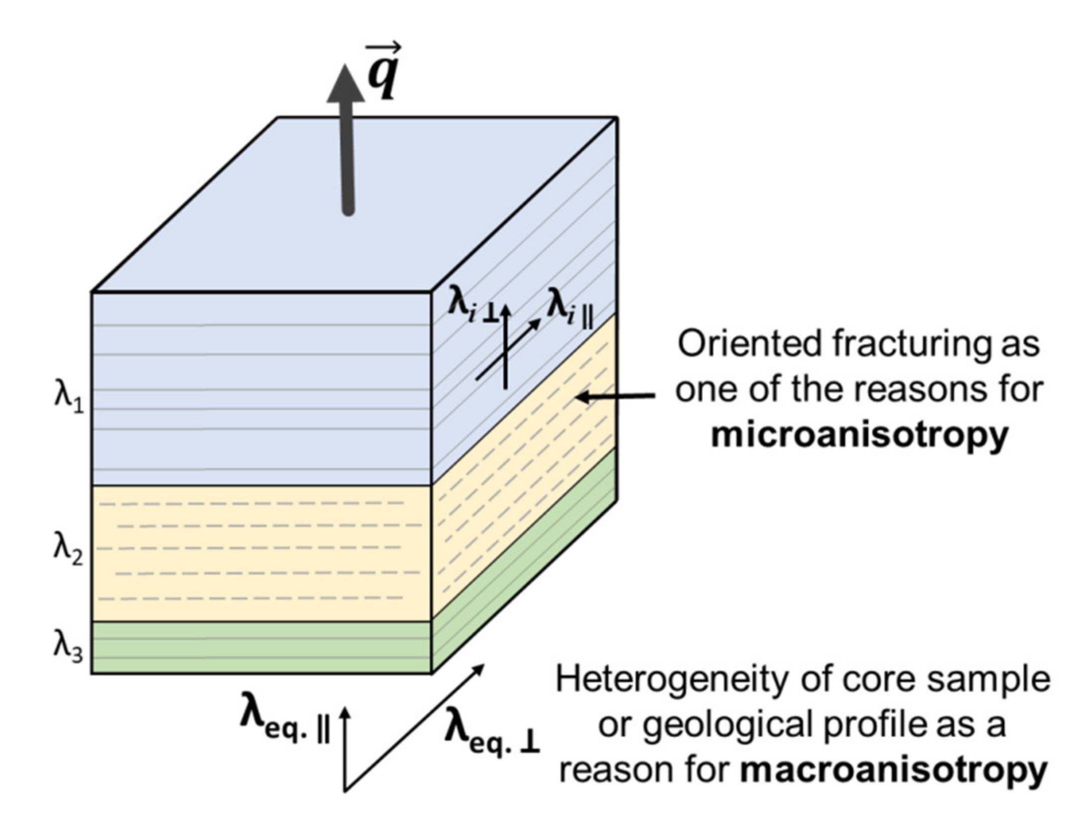
• The thermal macro-anisotropy due to the heterogeneity of rocks on the core sample scale (Figure 4)—a layered texture at the scale of the whole profile conditioned by the alternation of subparallel layers with various thermal conductivities;
• The micro-anisotropy inherent even for homogeneous rocks and caused either by oriented anisotropic mineral grains or oriented microcracks (Figure 4).

The analysis of the micro-anisotropy based on continuous thermal core logging data reveals the absence of significant anisotropy for limestones and dolomites (Table 3) but high values of thermal anisotropy coefficients for argillites, shaly siltstones, and quartz sandstones.

Table 4. Results of the experimental determination of the equivalent thermal conductivity along the vertical axis of the well under study for the investigated depth intervals using the results of the continuous thermal core logging of full-sized cores in an “as-received” state and atmospheric conditions.

Depth Interval, m	Upper-Bound Estimate λequiv.U, W⋅m−1⋅K−1	Lower-Bound Estimate λequiv.L, W⋅m−1⋅K−1	Average and Standard Deviation of λ‖, W⋅m−1⋅K−1	Average and Standard Deviation of λ⊥,W⋅m−1⋅K−1	Coefficient of Micro-anisotropy, KT = λ‖·λ⊥−1	N
1348.50–1366.10	2.38	2.24	2.52 (0.74)	2.40 (0.45)	1.06	135
2612.29–2629.20	2.11	2.02	2.15 (0.37)	2.07 (0.39)	1.04	145
2657.00–2665.74	2.30	2.23	2.32 (0.25)	2.26 (0.28)	1.03	73
2737.30–2746.02	2.51	2.33	2.54 (0.30)	2.38 (0.33)	1.08	78
2754.90–2763.60	2.43	2.35	2.44 (0.14)	2.36 (0.18)	1.03	65
2794.90–2812.50	2.42	2.31	2.43 (0.18)	2.34 (0.33)	1.04	143
2916.90–2934.34	2.52	2.44	2.54 (0.19)	2.47 (0.23)	1.03	143
3506.40–3539.30	2.33	2.09	2.41 (0.60)	2.19 (0.59)	1.11	272
3585.38–3597.40	4.09	3.19	4.15 (0.53)	3.38 (0.76)	1.28	92
3619.20–3630.68	2.57	2.46	2.65 (0.55)	2.56 (0.59)	1.05	89
3650.00–3667.08	2.65	2.38	2.66 (0.16)	2.46 (0.38)	1.11	93
3756.70–3776.31	3.12	2.56	3.25 (0.62)	2.73 (0.67)	1.24	148
3782.64–3812.12	2.80	2.30	2.81 (0.15)	2.37 (0.32)	1.20	223

contains the results of the equivalent thermal conductivity calculation for the investigated depth intervals using the results of continuous thermal core logging of all recovered full-sized cores. Due to the lack of reliable information about the presence or absence of the induced technogenic anisotropy for the investigated core samples (which is a common cause of anisotropy), two cases were considered:

• The equivalent thermal conductivity λ_U was determined according to Formula (5), assuming that the micro-anisotropy was caused by technogenic fractures (directed in most cases parallel to the bedding plane) and has to be excluded from the estimation of the in situ thermal conductivity of the rock mass, and because of that, the thermal conductivity parallel to the bedding plane (λ_‖) is a more objective and unbiased characteristic of the core sample compared to the thermal conductivity perpendicular to the bedding plane (λ_⊥) affected by micro-cracks (see in [11], Figure 4). For that reason, an upper-bound estimate of rocks’ thermal conductivity was made.
• The equivalent thermal conductivity λ_L was determined using Equation (4) assuming that the micro-anisotropy is typical for core samples at in situ conditions; i.e., it is caused by natural factors and corresponds to undisturbed rocks. For that reason, a lower-bound estimate of thermal conductivity was made.

The increase in the micro-anisotropy coefficient with depth (from the average of 1.04 in the 1348.50–2934.34 m depth interval to the average of 1.17 in the 3506.40–3812.12 m depth interval) provides evidence of the technogenic nature of anisotropy, since it is known that the decompression effect, which causes microcracks along parallel directions to the bedding plane, is higher for core samples recovered from deeper depth intervals [38].

Table 4 shows that to depths of 3000 m, the difference between λ_equiv.U and λ_equiv.L does not exceed 8%, with an average difference of 4.7%. However, for depth intervals below 3000 m, this difference reaches up 22–28% with an average difference of 16.5%, which is quite significant. It is important that the relative difference between λ_equiv.U and λ λ_equiv.L

$$\delta \lambda =\frac{{\lambda }_{equiv.U}-{\lambda }_{equiv.L}}{{\lambda }_{equiv.L}}$$

(5)

correlates with the average micro-anisotropy coefficient (K = λ_‖·λ_⊥) obtained from measurements on core samples along the orthogonal scanning lines (Table 3): δλ = 0.979⋅K − 0.975, the correlation coefficient is 0.995.

In most cases, to determine the heat flow density, researchers do not calculate the equivalent thermal conductivity along the well via Equations (5) and (6) but rather calculate its average values using the results of measurements on core samples [15]. However, it is more physically correct to calculate the thermal conductivity according to Equations (5) and (6) [3], since the average thermal conductivity, in this case, has the physical sense of the equivalent thermal conductivity of the heterogeneous rock mass for the horizontal direction of the heat flow. Table 4 contains average values of λ_‖ and λ_⊥. They differ from λ_equiv.U and λ_equiv.L for the studied rock mass by up to 5.9% and 7.1%, respectively. The relative difference δλ between λ_‖ and λ_equiv.U correlates with the standard deviation of λ_‖ (Table 4). The established regression equation is δλ = 0.141⋅SD² − 0.0379⋅SD + 0.078, with a determination coefficient of 0.936. Table 4 shows that the greatest deviation that can occur when calculating the equivalent thermal conductivity using the simplified method of the weighted arithmetic mean is 30.1% (in a 3585.38–3597.40 m depth interval). The average deviation for all intervals is 12.2%.

Figure 7 plots the estimates for the relative uncertainty in equivalent thermal conductivity data for the studied depth intervals at various core sampling rates along the well. Apart from the continuous core sampling that was realized during the thermal core logging of all full-sized cores (corresponding to a ~0.1 m sampling rate in our case, since the average length of studied core samples was about 99 mm), the estimates of the equivalent thermal conductivity data uncertainty were also made for 0.7 m, 1.5 m, and 3 m sampling steps. As an example, for all these sampling steps, the relative errors (δλ) in estimates of the average value of the equivalent thermal conductivity (λ_equiv.U) were calculated within each investigated depth interval (Table 1) with an estimation of the root-mean-square values (σ) for the obtained data populations within each studied depth interval using the Student’s coefficient t (for 0.95 confidence level) and sample size (N) for each depth interval for every sampling step. The formula for estimating the relative uncertainty of the average value estimate has a known form [11]:

$$\delta \lambda =\frac{\sigma ·t_{0.95}}{\langle \lambda \rangle ·\sqrt{N}}$$

(6)

The data in Figure 7 demonstrate that the continuous core selection for thermal property measurements in our studies provided us with the equivalent thermal conductivity estimates with a relative error ranging from 1.5–7% (depending on the depth interval). If the core sampling step was 0.7 m, the δλ error increased to 2.5–18%, if the step was 1.5 m, the error increased to 3–33%, and if the step was 3 m, the error increased to 5–93%. It should be noted that these error ranges are the lower-bound estimates of errors of heat flow determination since the error in data on temperature gradients (due to diverse reasons, including instrumental factors, insufficient recovery of the thermal equilibrium in the well, possible heat and mass transfer processes in borehole annulus, etc.) is added to the error in the equivalent thermal conductivity. This means that even with 0.7 m, 1.5 m, and 3 m core sampling steps, the uncertainty in the heat flow estimate for specific depth intervals (that were drilled with coring) reaches 18, 33, and 93%, correspondingly. As a result, there is no opportunity to investigate vertical variations of heat flow density within certain depth intervals due to excessive uncertainties.

Thus, the obtained estimates show that the continuous thermal core logging of all available cores is required to obtain the appropriate data on the thermal properties of rock and heat flow accounting for their vertical variations. At the same time, the registration of these data is a foundation for the methodology of today’s experimental geothermics [4,6,8].

3.4. Determining the Equivalent Thermal Conductivity within Non-Coring Intervals

The thermal conductivity of rock was determined from well-logging data based on regression analysis for limestones in depth intervals of 1992.4–2090.1 m, 2629.16–2720.9 m, 2721.16–2916.36 m, and 2935.16–3249.36 m. In addition to that, the thermal conductivity of rock was determined for dolomites in the 2145.36–2359.56 m depth interval based on the results of the regression analysis of well-logging data and data on thermal conductivity from the adjacent well that had a similar geological profile. Target intervals for predicting thermal conductivity were selected accounting for (1) available experimental data on thermal conductivity, (2) lithology and stratigraphy, and (3) quality of well-logging data.

Before regression analysis between well-logging data and data on the thermal conductivity of rocks, data preprocessing was conducted. The data preprocessing included (1) matching depths of logging curves, (2) eliminating data from cavernous intervals, (3) averaging the continuous thermal conductivity profile in a 0.5 m moving window (the window size is equal to the average vertical resolution of well-logging tools), and (4) shifting the core depth to match well-logging data using results of core gamma spectrometry. In addition to that, the Z-scaling (dividing the difference between a variable and its average value by its standard deviation) of neutron gamma logging and gamma-ray log data was performed to account for differences in the technical conditions of well-logging (drilling agent properties, well diameter, etc.) and logging tools when predicting the thermal conductivity of the dolomites in the 2145.36–2359.56 m depth interval.

The well-logging suite that was used to predict the rock thermal conductivity included the gamma-ray log, neutron gamma log, gamma–gamma density log, and sonic log. The thermal conductivity of rock was determined within non-coring intervals based on the multiple regression analysis of well-logging data and data on the thermal conductivity of rock. During the regression analysis, the outlier-resistant linear regression model (also known as Huber regression) presented in [39] was used. The loss function of the Huber regression contains two parameters (w and σ) that are optimized during model training and it is not heavily influenced by the outliers while accounting for their effect. The initial dataset of thermal conductivity data for rocks and well logging data was divided into the training dataset (67% of the entire dataset) and the test dataset (33% of the data set) to estimate the generalization ability of the determined regression equations. Optimal hyper-parameters of regression models were selected via the cross-validation method. The quality of thermal conductivity predictions for rocks from well-logging data was estimated on the test dataset via the root-mean-squared error (RMSE), the correlation coefficient between measured and predicted values, prediction precision (P), and accuracy (A) (see the corresponding formulas in [17]). Prediction precision characterizes the random component of uncertainty, and prediction accuracy refers to the systematic component. The correlation coefficient between the measured and predicted values provides an unbiased evaluation of the regression model fit on the training dataset.

The results of training and testing regression models for determining the thermal conductivity of rock from well-logging data are presented in

Table 5. The results of training and testing regression models for determining rock thermal conductivity from well-logging.

Lithology (Depth Interval)	Regression Equation *	Quality of Prediction Results on the Test Dataset
		r	RMSE, W·m−1·K−1	P, %	A, %	N
Limestones (2611.76–2665.76)	λ = −2.6·10−4·ΔtP + 0.25·ρ + 0.26·γ + 0.34·NGR + 0.08	0.84	0.10	9.48	−0.2	43
Limestones (2736.96–2812.16)	λ = −3.7·10−4·ΔtP + 0.12·ρ + 0.05·γ + 0.21·NGR + 2.15	0.43	0.10	8.06	−0.4	67
Limestones (2916.56–2934.16)	λ = −1.8·10−4·ΔtP − 0.25·γ + 0.32·NGR + 2.44	0.80	0.10	8.74	0.5	29
Dolomites (regression equation from the adjacent well)	λ = −0.004·γnormilized + 0.42·NGRnormalized + 4.34	93	0.17	8.18	0.2	133

* Δt_P—travel time of p-wave, ρ—rock density, γ—gamma-ray radioactivity, NGR—neutron gamma-ray log.

.

Based on the Pearson correlation test, the obtained values of the correlation coefficients were statistically significant for the 0.95 confidential probability level. Figure 8 plots the predicted rock thermal conductivity within non-cored intervals from well-logging data. Based on Table 5, it can be concluded that the established regression equations between well-logging data and data on rock thermal conductivity provide the predictions of rock thermal conductivity with a total uncertainty of less than 10% for a 0.95 confidence level.

The total length of the intervals with predictions of rock thermal conductivity from well-logging data was 860 m.

3.5. Estimating the Effect of Core Drying in Core Storage

Additional measurements of thermal properties that were conducted on 19 cylindrical core plugs with a diameter and length of 30 mm at different saturations (“as received”, dry, and water-saturated) included the following stages:

• measurements of core samples at atmospheric conditions immediately after drilling them out of the full-sized core samples;
• drying samples following the standard procedure in the drying box;
• measurements of the dried core samples at atmospheric conditions;
• vacuum saturation of core samples with mineralized water following the standard procedure;
• measurements on the water-saturated samples at atmospheric conditions;
• measurements of thermal conductivity of rock, volumetric heat capacity, and thermal anisotropy coefficient on water-saturated samples at in situ temperature (the temperature of measurements corresponds to the in situ temperature of the corresponding core sample).

Figure 9 plots the estimates of the relative variations of thermal conductivity (1) after drying and (2) after the saturation with synthetic brine under vacuum. The measurement results in Figure 9 show the following:

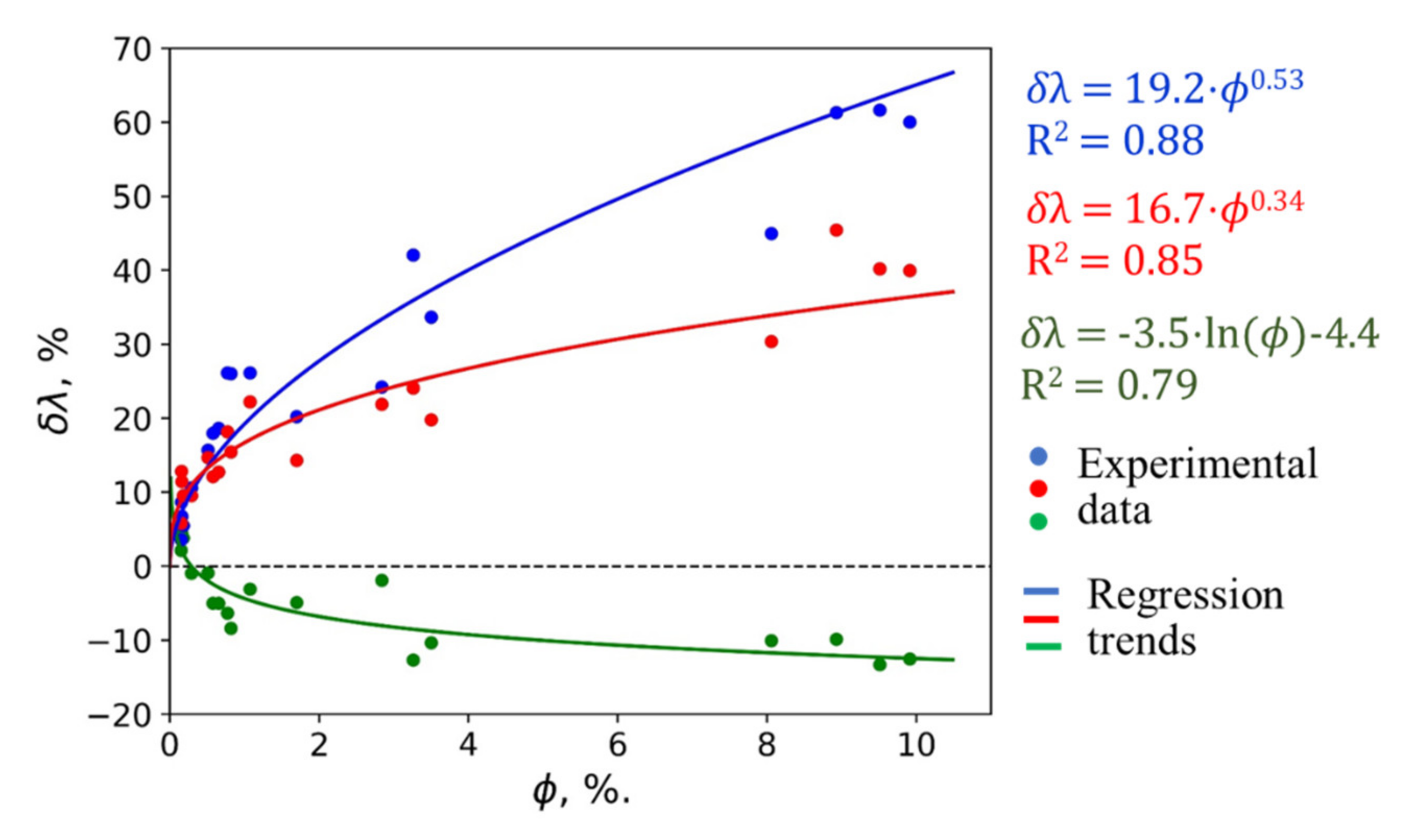
• The degree of thermal conductivity change after both drying and water saturation depended on the core sample porosity.
• The drying of the obtained samples resulted in a very small thermal conductivity decrease. The degree of thermal conductivity reduction depended on the porosity and does not exceed 13%.
• After the water saturation of the dried core samples, a substantial thermal conductivity increase was observed (from 7% to 62%).

There was no dependence established for the anisotropy degree of core samples from thermal conductivity variations during the change of pore-filling fluid.

The data in Figure 9 allow us to conclude that by the time of thermal core logging in the core storage, the samples were dried substantially and lost the majority of their pore fluid. Therefore, to correct the data on rock thermal conductivity for in situ saturation, it was necessary to adjust the results of thermal core logging depending on rock porosity via the regression trend presented by the red-colored curve in Figure 9. A. Duchkov et al. (2014) pointed out that the need for the water saturation of samples was largely neglected in past geothermal investigations, which led to systematic errors (up to 20–40%) in data on thermal conductivity and subsequently to at least the same severity errors in data on heat flow [12].

Variations of the rock thermal conductivity perpendicular to the bedding plane depending on porosity during changes of the sample saturation are described by regression equations that are similar to those for the thermal conductivity parallel to the bedding plane and are as follows:

• from “as received” state to dried: δλ = −3.5·ln(Φ) − 4.4 with R² = 0.79;
• from dried to water-saturated: δλ = 19.2·Φ ^0.53 with R² = 0.88;
• from “as received” state to water-saturated: δλ = 16.7·Φ ^0.34 with R² = 0.85.

Using the data within coring intervals on rock porosity that were obtained via interpreting the density log data and the results of laboratory investigations of core plugs, for each depth interval and for specific depth intervals that have significant porosity variations, using the regression equation corresponding to the red curve in Figure 9, the corrections for data on the thermal conductivity of rock (inferred from the continuous thermal core logging) were determined. It was necessary to obtain the valid thermal conductivity data for in situ conditions within the corresponding depth intervals (

Table 6. Thermal conductivity corrections to account for in situ saturation.

Depth Intervals, m	Average λeq, W·m−1·K−1	Average Porosity, %	Thermal Conductivity Correction for In Situ Saturation, %
For coring depth intervals
1348.50–1366.10	*	10.9	38
2612.29–2629.20	*	9.2	36
2657.00–2665.74	*	8.5	35
2737.30–2746.02	*	4.4	28
2754.90–2763.60	*	4.8	28
2794.90–2812.50	*	5.3	29
2916.90–2934.34	*	8.2	34
3506.40–3539.30	*	2.8	23
For intervals with well-log-based predictions of rock thermal conductivity
1991–2091	2.26	11	38
2144–2361	4.30	3	24
2628–2658	1.98	9	35
2666–2737	2.26	6	31
2764–2794	2.43	3	24
2813–2915	2.32	3	24
2935–3100	2.49	2	21

* within coring intervals, we deal with the upper and lower estimates of λ_equiv. See Table 4.

). The significant degree of the established corrections was caused not only by open porosity but also by the presence of micro-cracks in core samples. These micro-cracks are known to contribute significantly to thermal conductivity variations, especially for dry samples, even though the volume of the pore space of micro-cracks is quite small.

3.6. Results of Measurements of Thermal Properties at In Situ Temperatures

Table 6 contains the results of determining the equivalent thermal conductivity along the vertical axis of the well for depth intervals with well-log-based predictions of the thermal conductivity of rock and the determined thermal conductivity corrections for in situ saturation.

Table 7. Temperature corrections for thermal conductivity that were obtained from measurements with DTC-300 and pressure corrections for thermal conductivity that were inferred from literature data [30,31], for coring depth intervals and for depth intervals with well-log-based predictions of thermal conductivity.

Depth Interval, m	The Range of the In Situ Temperature, °C	Temperature Correction for Thermal Conductivity, %	Pressure Correction for Thermal Conductivity, %
For coring depth intervals
1348.50–1366.10	24.4–24.8	0	4
2612.29–2629.20	47.9–48.4	−4	6
2657.00–2665.74	49.1–49.3	−4	6
2737.30–2746.02	50.9–51.1	−4	6
2754.90–2763.60	51.3–51.5	−3.5	7
2794.90–2812.50	52.3–52.7	−3.5	7
2916.90–2934.34	55.1–55.5	−5	7
3506.40–3539.30	68.2–69.1	−7	7
For intervals with well-log-based predictions of rock thermal conductivity
1991–2091	35.84–38.14	−2	5.5
2144–2361	39.27–42.20	−2.5	6
2628–2658	48.35–49.10	−4	6
2666–2737	49.30–50.93	−4	6
2764–2794	51.54–52.26	−3.5	7
2813–2915	52.68–55.02	−3.5	7
2935–3100	55.48–59.24	−5	7

contains the corrections for in situ pressure and temperature for the thermal conductivity data that were inferred from measurements on standard cylindrical core plugs (of 50 mm diameter and 20 mm height) at the formation temperature with the DTC-300 device. The thermal conductivity at the formation temperature was measured on 10 cylindrical 50 × 20 mm core samples that were saturated with synthetic brine under vacuum and selected based on the results of the continuous thermal core logging of full-sized cores. Thermal conductivity measurements on water-saturated samples were conducted at the temperature that corresponded to the temperature of the corresponding depth interval. Pressure corrections for thermal conductivity were inferred from the literature data for the rocks that were similar to those presented in the investigating geological profile [30,31].

The results of the determination of the thermal conductivity decrease for various depth intervals (depth intervals at which the thermal conductivity was determined experimentally via measurements on core samples and for depth intervals with thermal conductivity predictions from well-logging data) during the increase in temperature from atmospheric to formation are provided in Table 7.

The rock volumetric heat capacity at formation temperatures was measured for 15 core samples that were selected based on the results of continuous thermal core logging. The measurement results revealed that increasing the temperature of core samples (presented by limestones and sandstones) from 25 °C to formation temperatures of 55–80 °C led to a 5–7% increase in rock volumetric heat capacity: from 2.20 and 2.35 MJ⋅m⁻³⋅K⁻¹ to 2.48 and 2,63 MJ⋅m⁻³⋅K⁻¹, corresponding to the established regression equation C(T) = −9·10⁻⁶·C² + 4.8·10⁻⁴·C + 2.08, which adequately characterizes the general pattern of the volumetric heat capacity increase with increasing temperature.

3.7. Determining Equivalent Thermal Conductivity at In Situ Conditions for Heat Flow Density Estimation

The equivalent thermal conductivity for the heat flow calculation was determined considering the multiscale rock heterogeneity (starting from each core sample), in situ saturation, the effect of core changes in core storage, textural anisotropy, micro-anisotropy, and in situ pressure and temperature.

Table 8. Results of determining equivalent thermal conductivity and heat flow density for coring depth intervals and intervals with well-log-based predictions of rock thermal conductivity within non-coring intervals.

Depth Interval, m	Estimation of Equivalent Thermal Conductivity, W⋅m−1⋅K−1		Temperature Gradient, mK⋅m−1	Heat Flow Estimate, mW⋅m−2
	Lower	Upper		Lower	Upper	Average
From results of continuous thermal core logging
1348.50–1366.10	3.21	3.42	18.05	58.0	61.7	59.8
2612.29–2629.20	2.80	2.93	28.30	79.3	82.8	81.1
2657.00–2665.74	3.07	3.17	23.93	73.5	75.8	74.6
2737.30–2746.02	3.04	3.28	22.72	69.1	74.5	71.8
2754.90–2763.60	3.11	3.22	24.68	76.8	79.5	78.1
2794.90–2812.50	3.08	3.23	22.08	68.1	71.3	69.7
2916.90–2934.34	3.33	3.44	23.00	76.7	79.2	78.0
3506.40–3539.30	2.57	2.87	27.56	70.8	79.0	74.9
From results of well-log-based predictions of rock thermal conductivity within non-coring intervals (average values of thermal conductivity and heat flow)
1991–2091	3.23		22.96	74.1
2144–2361	5.54		13.51	74.8
2628–2658	2.74		24.63	67.4
2666–2737	3.02		22.76	68.7
2764–2794	3.13		23.62	73.9
2813–2915	2.99		22.98	68.6
2935–3100	3.08		22.75	70.1

provides the results of the equivalent thermal conductivity calculation at in situ conditions for coring depth intervals and depth intervals with well-log-based predictions.

The vertical variations of the heat flow density presented in Table 8 are plotted in Figure 10 together with the previously published data on the average heat flow estimates that were inferred from [10,40,41].

4. Discussion

4.1. Reasons of Vertical Variations in Thermal Properties of Rock

The terrigenous sediments of the Bavlinsky suite (sandstones, aleurolites, gravelites) are characterized by lower thermal conductivity values (by 23–27%) and by lower thermal heterogeneity coefficient (by 35–59%) compared to the terrigenous rocks of the Koyvensky horizon. The differences in thermal conductivity are conditioned by the difference in mineral composition; i.e., the presence of relatively poorly heat-conducting rock-forming minerals, such as mica, field-spars, clay minerals (1.8–2.6 W·m⁻¹·K⁻¹ [37]) in the deposits of the Bavlinsky suite. The deposits of the Bavlinsky suite on the strata scale have high thermal conductivity in a parallel direction to the bedding plane, as evidenced by a relatively low standard deviation value (standard deviation is 0.15 W·m⁻¹·K⁻¹) for thermal conductivity parallel to the bedding plane (Table 3). The average values of the thermal anisotropy coefficient are quite similar for the terrigenous deposits of the Koyvensky horizon and the Bavlinsky suite, which is associated with the textural features of the rocks. In the sediments of the Koyvensky horizon, there are intervals of the rhythmic thin-bedded interlayering of mid- and coarse-grained sandstones, mid- and fine-grained sandstones, and argillites. There are also intervals of rocks with a thin-layered texture due to an argillaceous–carbonaceous material with muscovite flakes. In the Bavlinsky sediments, thin-bedded textures with numerous muscovite flakes can be seen along the bedding direction (a high thermal anisotropy characterizes the muscovite monocrystal: λ_c = 1.03–1.07 W·m⁻¹·K⁻¹; λ_a,b = 3.80–3.55 W·m⁻¹·K⁻¹ [37]). The variations of the thermal conductivity, the volumetric heat capacity of limestone, and thermal heterogeneity coefficient are due to varying degrees of dolomitization (uneven, spotty dolomitization, weak and intense), silicification (spotty), oil saturation (uneven, weak, etc.), clay content in rock, and porosity variations. The investigated limestones are poorly anisotropic (K_T = 1.03–1.08). Argillite interlayers that typically exhibit thermal anisotropy cause an increase in the average values of the thermal anisotropy coefficient (up to 1.11) for deposits of Biysk and Mullino horizons. The high thermal heterogeneity on the strata scale of the Artinsk and Vorobyev horizon deposits (with thermal conductivity standard deviation varying from 0.59–0.72 W·m⁻¹·K⁻¹) is conditioned by the interlayers of highly heat-conductive anhydrite at the top of the Artinsk deposits (1347.80–1349.15 m), highly heat conductive dolomites at the bottom part (1362.25–1363.40 m), and interlayers of highly heat-conductive quartz sandstones in the Vorobyev horizon within a 3624.11–3625.06 m depth interval.

4.2. Analysis of the New Heat Flow Data

The average heat flow density for 13 depth intervals between 2144 and 3539 m (Table 8) is 72.6 mW·m⁻² with a standard deviation of 3.6 mW·m⁻². For 13 sampling elements and the corresponding Student’s coefficient of 2.16 at the 0.95 confidence level, the absolute uncertainty of the estimate of the average heat flow density is 2.2 mW·m⁻², whereas the relative uncertainty of the estimate of the average heat flow density is 3.0%.

The most severe variations of heat flow density probably do not reflect the experimental uncertainty but rather characterize the specifics of heat and mass transfer processes in the rock mass. Another possible reason could be the variations of rock mass properties at a particular distance from the investigating well.

The highest discrepancies between upper and lower estimates of the heat flow density are observed for 1348.50–1366.10 m, 2737.30–2746.02 m, and 3506.40–3539.30 m depth intervals. For these intervals, the measurement results revealed the highest anisotropy of the thermal conductivity of rock (with micro-anisotropy coefficients of 1.06, 1.08, and 1.11, respectively; see Table 4) that cannot be reliably classified as natural or induced, as previously stated (in Section 3.3).

The results of determining the heat flow density for the 2612–2629 m depth interval were not considered when assessing the average heat flow density, since this depth interval has anomalously high values of the temperature gradient (Figure 10). This may not reflect the actual behavior of the conductive component of the heat flow density; rather, it may reflect a consequence of local movements of fluid in the inner annulus or be caused by the abnormal operation of the measurement tool in this interval. The estimates of heat flow density for the 3585.38–3597.40 m depth intervals are not reported for the same reason.

Although thermal conductivity data for the depth intervals below 3539.30 m (Table 3 and Table 4) were not used within our research to determine the heat flow density, these results are important for the basin modeling of the area under study and, for this reason, they are included in this paper. Moreover, the Volga–Ural basin territory may have granite intrusions (or metamorphic rocks formed as a result of their processing) “which transmit well hot hydrothermal solutions during neotectonic transformation, and, due to high thermal conductivity, create favorable conditions for oil-source rock maturation and development of secondary reservoirs” [23].

4.3. Comparison of the New Heat Flow Estimates with Previous Data

The previously published data contain geothermal information for seven wells in the drilling area: Orenburg, [40], two unnamed wells [41], Goncharovskaya-16, Denisovskaya-1, Denisovskaya-3, and Yakshimbetovskaya-157 [10] (see Figure 1, red dots). These wells are 118, 87, 38, 118, 130, 103, and 113 km away from the studied well, respectively. The published heat flow estimates for these wells are 48, 38, 26 32, 33, 31, and 30 mW·m⁻², respectively, with an average heat flow density of 34.0 mW·m⁻².

For the first three wells (Orenburgskaya and two unnamed wells), there is no information in the publications [40,41] on the depth of investigations, well suspension, methods of estimating the equilibrium temperature gradient, and the thermal conductivity of rock. For three of the last four wells, there are data on well suspension, and for one well, the well was suspended for one week, which is obviously insufficient to achieve thermal equilibrium in the rock mass after drilling [10]. The average rock thermal conductivity was only estimated based on descriptions of geological sections and using data from other areas (the data for specially collected samples from wells located southwest of the East European Platform [10] were used), since drilling was without coring. The peculiarities of the conducted geothermal experiments in these seven wells should result in substantial differences between our data on heat flow density and the previously published values.

When estimating the deep heat flow density using literature data, it should be considered that almost all previous studies had the following specifics:

• The conductive component of the heat flow density was commonly calculated using the average values of thermal conductivity and temperature gradient along the wells, excluding the possibility of substantial vertical variations of the heat flow density below 300–500 m [3,10,15];
• For 80% of the investigated wells, no measurements of rock thermal conductivity were conducted, whereas the data on rock thermal conductivity were inferred from the literature data for similar rocks [10];
• In the case of experimental measurements of rock thermal conductivity, devices designed for measurements on industrial materials were applied [11]; usually, they do not allow the reliable estimation of the anisotropy and heterogeneity of rock and provide a significantly underestimated thermal conductivity of rock due to the strong effect of thermal contact resistance between the rock sample and the measurement probe [11];
• Most thermal conductivity measurements were conducted without the mandatory water saturation of core samples, which resulted in results for the thermal conductivity measurements for sedimentary and fractured rocks that were underestimates by 20–40% [12] and did not account for the technogenic decompaction of rock samples that can be caused by the decompression effect, drilling equipment impact, and mechanical treatment of core samples required by traditional methods and measurement devices [11];
• The heat flow estimations were conducted for shallow wells (about 70% of wells were less than 1500 m deep) assuming a stable value of heat flow below 300–500 m (considering the negligible effect of radiogenic heat generation);
• In most cases, it was impossible to conduct the temperature logging in wells that reached the thermal equilibrium in rock masses after drilling.

Each of the above-mentioned factors usually results in the underestimation of heat flow density. In combination, those factors resulted in an underestimation of the deep heat flow density by 40–140%, which was convincingly demonstrated by geothermal studies of deep and super-deep scientific continental wells drilled in the USSR, Russia, and other countries [4,5,6,7,8,9,13,16,25,42].

The quality of the previous data on heat flow density in the investigated area may not be considered even as satisfactory, since none of the following mandatory requirements for geothermal investigations (Popov, 2015) were fulfilled: temperature measurements in steady-state wells, experimental measurements of rock thermal conductivity on a representative collection of core samples accounting for in situ conditions, accounting for vertical variations of the temperature gradient and rock thermal conductivity, and registration of vertical variations of heat flow.

Figure 10 demonstrates that all the newly obtained data on heat flow density are significantly higher than the average value of previously published data. The heat flow density for the 1348.50–1366.10 m depth interval varies from 58.0 to 61.7 mW·m⁻² with an average value of 59.8 mW·m⁻², which is essentially lower than the heat flow density for the deeper horizons (below 1991 m). This is coherent with the previously determined tendency, suggesting that the heat flow density for depths less than 2000 m is in most cases smaller than the heat flow density for deeper depths due to the combined impact of the paleoclimate and migration of fluids in rock masses [4,5,6,7,8,9,13,16,25,42].

Thus, the obtained average heat flow value within the depth intervals below 2000 m could be considered as undisturbed terrestrial heat flow density, which is greater than the previous heat flow average value for this territory by 114%.

The large difference between previous and new data on the heat flow for the area studied can be explained by the following factor:

• The thermal property measurements of rock without comprehensive brine saturation results in the underestimation of the measured thermal conductivity by 20–40%, leading to heat flow underestimation by 20–40% [12].
• The influence of thermal resistance between the measuring instrument components and rock sample surfaces in thermal conductivity measurement results leads to heat flow underestimation, usually by 10–30% for crystalline rocks and 15–40% for sedimentary rocks, according to [11] and our long-term experimental experience.
• The temperature measurements in wells that did not reach thermal equilibrium cause an underestimation in temperature gradient that leads to heat flow underestimation (up to 20–30%) according to our long-term temperature measurements in scientific wells.
• Previous practice with averaging temperature gradient causes an underestimation of the temperature gradient that leads to heat flow underestimation;
• The influence of the paleoclimate effect when the measurements are performed in wells with a depth less than 1 km leads to heat flow underestimation, usually by 5–10% [25].

All these effects exceed the influence of radiogenic heat generation on heat flow variations within the depth intervals under study. The radiogenic heating caused by the spontaneous decay of the radioactive elements contained in sediments was estimated in the interval 2524–3827 m based on the results of spectral gamma-logging in the well (the concentration of uranium, thorium, and potassium) using the approach suggested by [43]. The calculated rock heat production rate for different layers varies from 0.6 up to 2.14 μW·m⁻³. Accounting for the actual data on porosity, this leads to an increase in heat flow value of about 1.2 mW·m⁻² within the considered interval of 1303 m of thickness. Thus, compared to the registered heat flow variations, the effect from radiogenic heat can be considered negligible.

The effect of the possible advection in formation could essentially sometimes influence the vertical heat flow variations [6,42]. Estimating the effect of advection requires special efforts and information on the formation and mass transfer processes in the area under study and is out of the scope of this paper.

4.4. Estimates of Paleoclimate Effect on Vertical Variations of Temperature Gradient and Heat Flow

It is known that, due to the thermal conductivity mechanism, surface temperature variations penetrate deep into the Earth with amplitude decay and delay, distorting the thermal field. Thus, to date, the temperature distribution in the upper layers of rock masses depends on the paleoclimate. To account for the effect of the paleoclimate on a measured heat flow density, reliable data on temperature behavior in the past on the Earth’s surface and data on rock thermal properties are required. The obtained experimental data on volumetric heat capacity and thermal conductivity were used to estimate the paleoclimate’s effect on vertical variations of heat flow.

Previously, during investigations of the southeast margin of the East European Platform (the well under study is located in this region), no corrections for the effect of the paleoclimate on heat flow data were made due to the absence of reliable data on the duration of climate epochs and the amplitude of the temperature change during these epochs [44]. The first attempt to introduce corrections for the effect of the paleoclimate on the registered heat flow density in that area was made by I. Kukkonen [13]. He used a simplified approach, where only the maximum depth of heat flow determination was considered, whereas the distribution of distortions caused by the effect of the paleoclimate is nonuniform in different depth intervals [25].

New paleo-surface temperatures were recently published [10,45], which allow the effect of the paleoclimate on the heat flow density to be accounted for. A climate change model considering spatial distribution patterns of surface temperature was suggested [25]. Based on this, the mathematical modeling of the disturbance of heat flow density and temperature gradient caused by climate change was conducted. A one-dimensional, time-dependent equation of thermal conductivity for a heterogeneous medium [46] was solved with the defined initial and boundary conditions during modeling. The data on regional paleoclimate (temperature on the surface) over the last 250 thousand years were used as the boundary condition on the Earth’s surface. Modeling results revealed that the most significant temperature gradient deviations were caused by the warming (approximately by 10 °C) that occurred at the end of the Ice Age about 10,000 years ago (Figure 11). The Little Ice Age (150–650 years ago) substantially affected the temperature gradient in the upper 400–500 m.

The temperature gradient deviations due to the paleoclimate are small and reach a maximum of 0.30–0.35 mK·m⁻¹ at a depth of 2200 to 2700 m, which is equivalent to a 1.3–1.6% deviation of the temperature gradient. This is equivalent to a quite small deviation of the heat flow density, which is not greater than 1–1.3 mW·m⁻². Above 1500 m, the temperature gradient disturbance is higher compared to the lower part of the well. The vertical variations of heat flow density (determined based on experimental geothermal investigations of the well) and the difference between new and old estimates of the heat flow density, which are 72.6 and 34 mW·m⁻², respectively, cannot be explained by the paleoclimate effect only. It is worth considering the possible effects of fluid migration [42]. The same situation was observed for the results of experimental geothermal investigations conducted for almost all deep and super-deep wells of the USSR, Russia, Germany, USA, and other countries [4,5,6,7,8,9,13,16,25,42].

4.5. Applying the Updated Geothermal Characteristics for Basin Modeling

An impact of the uncertainty of thermal conductivity and heat flow density on the results of sedimentary basins and petroleum system modeling is beyond dispute among specialists [47,48]. However, corresponding estimates obtained with reliable geothermal data are rarely published (see, e.g., [2] and references therein). Two variants of the 1D model of the investigated sedimentary basin (which are distinct in their geothermal parameters, and both were successfully calibrated on temperature data and vitrinite reflectance data) were constructed to demonstrate the impact on the degree and volume of organic matter transformation (see details in [24]). In the first variant of the model, which is in good agreement with the past estimates of heat flow data, the thermal conductivity of rock is calculated using data on the established lithology and thermal conductivity of the rock components [1] accounting for the in situ temperature [49]. In the second variant of the model, geothermal data are taken from the results of actual experimental investigations. The comparison of the calculation results obtained for the two model variants demonstrated that the use of reliable geothermal data allowed the more accurate determination of the degree of organic matter transformation (27% instead of 37% at this very moment), as a result increasing the accuracy of data on the mass of the generated organic matter by ~27%.

5. Conclusions

An investigation of more than 1700 rock samples was conducted with new techniques, including continuous thermal core logging, new laser optical scanning instrument, and the well-log-based prediction of rock thermal conductivity, in combination with rock thermal property measurements at elevated temperatures and on core samples saturated under vacuum with brine.

The conducted investigation provided representative experimental data on the thermal properties of rock, including thermal conductivity components along and perpendicular to the rock bedding plane, the volumetric heat capacity, and the anisotropy coefficient for determining heat flow density, in 14 depth intervals along the well that crossed the Domanik Formation.

According to the measurement results for 16 depth intervals between 2144 m and 3539, the average heat flow density is 72.6 ± 2.2 mW·m⁻². The heat flow density increases with depth in the 1350–2144 m depth interval from 59.6 mW·m⁻² (the value is given with an uncertainty not larger than ±10%) to 72.6 mW·m⁻²; i.e., by 22% from 1350 to 2144 m. The average value of the heat flow density exceeds the previously published value for this area (34 mW·m⁻², [10,39,40]) by 114%.

The large difference between previous and new data on the heat flow for the district studied can be explained by the following reasons:

• The thermal property measurements of rock without comprehensive brine saturation results in the underestimation of the measured thermal conductivity by 20–40%, which leads to heat flow underestimation by 20–40%.
• The influence of thermal resistance between the measuring instrument components and rock sample surface results in thermal conductivity measurement results that usually lead to heat flow underestimation by 10–30% for crystalline rocks and 15–40% for sedimentary rocks.
• The temperature measurements in wells that did not reach thermal equilibrium cause an underestimation of the temperature gradient that leads to heat flow underestimation (up to 20–30%).
• Previous practice with averaging temperature gradient causes an underestimation of the temperature gradient that leads to heat flow underestimation (10–20% for lower horizons).
• The influence of the effect of the paleoclimate when the measurements are performed in wells with a depth less than 1 km leads to heat flow underestimation, usually by 5–10%.

As shown by experimental geothermal investigations in deep and super-deep wells conducted between 1990 and 2010, the difference between obtained and previously published data on heat flow and rock thermal properties demonstrated the necessity for new, special experimental estimations.

The results of our research are crucial for studying hydrocarbon fields at any stage, including regional basin and petroleum system modeling.

References

1. Hantschel, T.; Kauerauf, A.I. Fundamentals of Basin and Petroleum Systems Modeling, 1st ed.; Springer: Berlin/Heidelberg, Germany, 2009; 476p. [Google Scholar]
2. Chekhonin, E.; Popov, Y.; Peshkov, G.; Spasennykh, M.; Popov, E.; Romushkevich, R. On the importance of rock thermal conductivity and heat flow density in basin and petroleum system modelling. Basin Res. 2020, 32, 1261–1276. [Google Scholar] [CrossRef]
3. Haenel, R.; Stegena, L.; Rybach, L. Handbook on Terrestrial Heat Flow Density Determination, 1st ed.; Springer: Dordrecht, The Netherlands, 1988; p. 486. [Google Scholar]
4. Clauser, C.; Giese, P.; Huenges, E.; Kohl, T.H.; Lehmann, H.; Rybach, L.; Zoth, G. The thermal regime of the crystalline continental crust: Implications from the KTB. J. Geophys. Res. 1997, 102, 18417–18441. [Google Scholar] [CrossRef]
5. Emmermann, R.; Lauterjung, J. The German continental deep drilling program KTB: Overview and major results. J. Geophys. Res. 1997, 102, 18179–18201. [Google Scholar] [CrossRef]
6. Popov, Y.; Pevzner, S.; Pimenov, V.; Romushkevich, R. New geothermal data from the Kola superdeep well SG-3. Tectonophysics 1999, 306, 343–366. [Google Scholar] [CrossRef]
7. Popov, Y.A.; Romushkevich, R.A.; Popov, E.Y.; Bashta, K.G. Results of Drilling and Investigating Super-Deep Ural Well; Nedra Publ.: Yaroslavl, Russia, 1999; pp. 77–88. [Google Scholar]
8. Kukkonen, T.; Rath, V.; Kivekas, L.; Šafanda, J.; Čermak, V. Geothermal studies of the Outokumpu Deep Drill Hole, Finland: Vertical variation in heat flow and palaeoclimatic implications. Phys. Earth Planet. Inter. 2011, 188, 9–25. [Google Scholar] [CrossRef]
9. Popov, Y.; Huddlestone-Holmes, C.; Gerner, E. Evolution in the reliability of experimental geothermal data. In Proceedings of the 2012 Australian Geothermal Energy Conference, Sydney, Australia, 14–16 November 2012. [Google Scholar]
10. Golovanova, I.V. Thermal Field of the Southern Urals; Nedra Publ.: Leningrad, Russia, 2005; 189p. [Google Scholar]
11. Popov, Y.; Beardsmore, G.; Clauser, C.; Roy, S. ISRM Suggested methods for determining thermal properties of rocks from laboratory tests at atmospheric pressure. Rock Mech. Rock Eng. 2016, 49, 4179–4207. [Google Scholar] [CrossRef]
12. Duchkov, A.D.; Sokolova, L.S.; Ayunov, D.E.; Zlobina, O.N. Thermal conductivity of sediments in high-latitude West Siberia. Russ. Geol. Geophys. 2013, 54, 1952–1960. [Google Scholar] [CrossRef]
13. Kukkonen, I.T.; Golovanova, I.V.; Khachay, Y.V.; Druzhinin, V.S.; Kosarev, A.M.; Schapov, V.A. Low geothermal heat flow of the Urals fold belt—Implication of low heat production, fluid circulation or palaeoclimate? Tectonophysics 1997, 276, 63–85. [Google Scholar] [CrossRef]
14. Demezhko, D.Y.; Golovanova, I.V. Climatic changes in the Urals over the past millennium—An analysis of geothermal and meteorological data. Clim. Past 2007, 3, 237–242. [Google Scholar] [CrossRef] [Green Version]
15. Stein, C.A. Heat Flow of the Earth. In Global Earth Physics: A Handbook of Physical Constants, 3rd ed.; Ahrens, T.J., Ed.; American Geophysical Union: Washington, DC, USA, 1995; pp. 144–158. [Google Scholar] [CrossRef] [Green Version]
16. Popov, Y.; Popov, E.; Chekhonin, E.; Spasennykh, M.; Goncharov, A. Evolution in information on crustal geothermal parameters due to application of advanced experimental basis. IOP Conf. Ser. Earth Environ. Sci. 2018, 249, 012042. [Google Scholar] [CrossRef]
17. Technically Recoverable Shale Oil and Shale Gas Resources: Russia. U.S. Energy Information Administration Report. Available online: https://www.eia.gov/analysis/studies/worldshalegas/pdf/Russia_2013.pdf (accessed on 25 March 2021).
18. Peterson, J.A.; Clarke, J.W. Petroleum Geology and Resources of the Volga-Ural Province, U.S.S.R.; USGS Geological Survey Circular; U.S. Geological Survey: Reston, VA, USA, 1983; 33p. [Google Scholar] [CrossRef]
19. Liang, X.; Jin, Z.; Philippov, V.; Obryadchikov, O.; Zhong, D.; Liu, Q.; Uspensky, B.; Morozov, V. Sedimentary characteristics and evolution of Domanik facies from the Devonian–Carboniferous regression in the southern Volga-Ural Basin. Mar. Pet. Geol. 2020, 119, 104438. [Google Scholar] [CrossRef]
20. Neruchev, S.G.; Rogozina, E.A.; Parparova, G.M.; Zelichenko, I.A.; Silina, N.P. Oil and Gas Formation in Deposits of the Domanik Type; Nedra Publ.: Leningrad, Russia, 1986; 248p. (In Russian) [Google Scholar]
21. Bazhenova, T.K. Hydrocarbon resources estimation of bituminous formations of Russian oil and gas bearing basins. Oil Gas Geol. 2017, 5, 37–50. (In Russian) [Google Scholar]
22. Ulmishek, G.F. Petroleum Geology and Resources of the West Siberian Basin, Russia; USGS Bulletin 2201–G; USGS: Denver, CO, USA, 2003; 53p. [Google Scholar]
23. Vashkevich, A.A.; Strizhnev, K.V.; Shashel, V.A.; Zakharova, O.A.; Kasyanenko, A.A.; Zagranovskaya, D.E.; Grebenkina, N.Y. Forecast of prospective areas for sediment type Domanic in the Volga-Ural oil and gas Province. Oil Ind. 2018, 12, 14–17. (In Russian) [Google Scholar] [CrossRef]
24. Chekhonin, E.; Popov, Y.; Vladimirov, A.; Spasennykh, M.; Zagranovskaya, D.; Zakharova, O. Improving the reliability of basin modeling results by enhancement of determination of geotherml characteristics and their integration into basin model. In Proceedings of the EAGE/SPE Workshop «Shale Science: New Challenges», Moscow, Russia, 5–6 April 2021. [Google Scholar]
25. Golovanova, I.V.; Puchkov, V.N.; Sal’manova, R.Y.; Demezhko, D.Y. A New Version of the Heat Flow Map of the Urals with Paleoclimatic corrections. Dokl. Earth Sci. 2008, 422, 1153–1156. (In Russian) [Google Scholar] [CrossRef]
26. Popov, E.; Goncharov, A.; Popov, Y.; Spasennykh, M.; Chekhonin, E.; Shakirov, A.; Gabova, A. Advanced techniques for determining thermal properties on rock samples and cuttings and indirect estimating for atmospheric and formation conditions. IOP Conf. Ser. Earth Environ. Sci. 2019, 367, 012017. [Google Scholar] [CrossRef]
27. Popov, Y.; Pimenov, V.; Pevzner, L.; Romushkevich, R.; Popov, E. Geothermal characteristics of the Vorotilovo deep borehole drilled into the Puchezh-Katunk impact structure. Tectonophysics 1998, 291, 205–223. [Google Scholar] [CrossRef]
28. Shakirov, A.; Chekhonin, E.; Popov, Y.; Popov, E.; Spasennykh, M.; Zagranovskaya, D.; Serkin, M. Rock thermal properties from well-logging data accounting for thermal anisotropy. Geothermics 2021, 92, 102059. [Google Scholar] [CrossRef]
29. Popov, E.; Popov, Y.; Chekhonin, E.; Safonov, S.; Savelev, E.; Gurbatova, I.; Ursegov, S.; Shakirov, A. Thermal core profiling as a novel and accurate method for efficient characterization of oil reservoirs. J. Pet. Sci. Eng. 2020, 193, 107384. [Google Scholar] [CrossRef]
30. Yakovlev, B.A. Prediction of Hydrocarbon Potential via Geothermal Data; Nedra Publ.: Leningrad, Russia, 1996; 240p. [Google Scholar]
31. Kurbanov, A.A. Regularities of Behavior of Thermophysical Properties of Fluid Bearing Reservoirs at In Situ Conditions and Its Applications. Ph.D. Thesis, Schmidt Institute of Physics of the Earth of the Russian Academy of Sciences, Moscow, Russia, October 2007. [Google Scholar]
32. Hohne, G.W.; Hemminger, W.F.; Flammersheim, H.J. Differential Scanning Calorimetry, 2nd ed.; Springer: Berlin/Heidelberg, Germany, 2003; pp. 154–196. ISBN 978-3-662-06710-9. [Google Scholar]
33. Standard Test Method for Determining Specific Heat Capacity by Differential Scanning Calorimetry. Available online: https://www.astm.org/Standards/E1269.htm (accessed on 25 April 2021).
34. Popov, Y.; Parshin, A.; Miklashevskiy, D.; Abashkin, V. Instrument for measurements of linear thermal expansion coefficient of rocks. In Proceedings of 46th US Rock Mechanics/Geomechanics Symposium, Chicago, IL, USA, 24 June 2012. [Google Scholar]
35. Willis, J. Bounds and self-consistent estimates for the overall properties of anisotropic composites. J. Mech. Phys. Sol. 1977, 25, 185–202. [Google Scholar] [CrossRef]
36. Meshalkin, Y.; Shakirov, A.; Popov, E.; Koroteev, D.; Gurbatova, I. Robust well-log based determination of rock thermal conductivity through machine learning. Geophys. J. Int. 2020, 222, 978–988. [Google Scholar] [CrossRef]
37. Popov, Y.; Berezin, V.; Soloviov, G.; Romuschkevitch, R.; Korostelev, V.; Kostiurin, A.; Kulikov, A. Thermal conductivity of minerals. Izv. Phys. Solid Earth 1987, 23, 245–253. [Google Scholar]
38. Popov, Y.; Pevzner, L.; Romushkevich, R.; Korostelev, V.; Vorobiev, M. Thermophysical and geothermal sections obtained from Kolvinskaya well logging data. Phys. Chem. Earth Part A Solid Earth Geod. 1994, 30, 778–789. [Google Scholar]
39. Huber, P.J.; Ronchetti, E.M. Robust Statistics Concomitant Scale Estimates; John Wiley & Sons, Inc.: Hoboken, NJ, USA, 2009; 172p. [Google Scholar]
40. Hodyreva, E.Y.; Shchulaev, V.F.; Netkach, A.Y.; Markov, A.I. Initial geothermal field of Orenburg gas-condensate field. Oil Gas Geol. 1985, 3, 43–48. (In Russian) [Google Scholar]
41. Gordienko, V.V.; Zavgorodskaya, O.V.; Moiseenko, U.I. Heat Flow Map of the Territory of the USSR. Scale 1:5,000,000. Explanatory Note. Kiev 1987-34 c. (In Russian)
42. Mottaghy, D.; Schellschmidt, R.; Popov, Y.A.; Clauser, C.; Romushkevich, R.A.; Kukkonen, I.T.; Nover, G.; Milanovsky, S. New heat flow data from the immediate vicinity of the Kola super-deep borehole: Vertical variation in heat flow confirmed and attributed to advection. Tectonophysics 2005, 401, 119–142. [Google Scholar] [CrossRef]
43. Rybach, L. Determination of heat production rate. In Handbook of Terrestrial Heat-Flow Density Determination; Kluwer: Philadelphia, PA, USA, 1988; pp. 125–142. [Google Scholar]
44. Sal’nikov, V.E. Geothermal Regime of the Southern Urals; Nedra Publ.: Leningrad, Russia, 1984; 88p. (In Russian) [Google Scholar]
45. Demezhko, D.Y.; Ryvkin, D.G.; Outkin, V.I.; Duchkov, A.D.; Balobaev, V.T. Spatial distribution of Pleistocene/Holocene warming amplitudes in Northern Eurasia inferred from geothermal data. Clim. Past 2007, 3, 559–568. [Google Scholar] [CrossRef] [Green Version]
46. Golovanova, I.V.; Selezneva, G.V.; Smordov, E.A. Reconstruction of postglacial warming in The Southern Urals using the 1242 temperature logging data. Geol. Sb. 2000, 1, 113–116. (In Russian) [Google Scholar]
47. Gallagher, K.; Ramsdale, M.; Lonergan, L.; Morrow, D. The role of thermal conductivity measurements in modelling thermal histories in sedimentary basins. Mar. Pet. Geol. 1997, 14, 201–214. [Google Scholar] [CrossRef]
48. Hicks, P.J.; Fraticelli, C.M.; Shosa, J.D.; Hardy, M.J.; Townsley, M.B. Identifying and quantifying significant uncertainties in basin modeling. In Basin Modeling: New Horizons in Research and Applications; Peters, K.E., Curry, D.J., Kacewicz, M., Eds.; AAPG Hedberg Series; AAPG: Tulsa, OK, USA, 2012; Volume 4. [Google Scholar]
49. Sekiguchi, K. A method for determining terrestrial heat flow in oil basinal areas. Tectonophysics 1984, 103, 67–79. [Google Scholar] [CrossRef]
Figure 2. Distribution histogram for the length of full-sized cores under study.
Geosciences 11 00346 g002
Figure 3. Workflow for determining heat flow density.
Geosciences 11 00346 g003
Figure 4. The reasons for the anisotropy of rocks that were accounted for during the determination of the equivalent thermal conductivity required to calculate the heat flow density. λeq.—macroanisotropy, λi—microanisotropy.
Geosciences 11 00346 g004
Figure 5. Temperature (left) and temperature gradient (right) along the well. Black dots on the left panel represent intervals of drilling with coring. Red dots on the right panel represent low well-quality-intervals (cavernous intervals; diameters of caverns exceed 10 cm). Dashed black line on the right panel represents the regression trend for temperature gradient with depth. Lithology legend: 1—sandstone, 2—carbonate-rich sandstone, 3—bituminous argillite, 4—clayous sandstone, 5—silty argillite, 6—limestone, 7—dolomite, 8—dolomite limestone, 9—limy dolomite, 10—anhydrite.
Geosciences 11 00346 g005
Figure 6. Results of continuous thermal core logging for depth intervals of 1348.5–1366.1 m (upper panel), 2612.29–2629.2 m (middle panel), and 2657.00–2665.74 m (lower panel). Black dots represent thermal conductivity parallel to the bedding plane, red dots show the thermal conductivity perpendicular to the bedding plane, green dots show the volumetric heat capacity, blue dots show the thermal heterogeneity factor, and purple dots represent the thermal anisotropy coefficient. Grey dots represent profiles with a 1 mm spatial resolution of thermal conductivity and volumetric heat capacity. Colored dots represent core scale data.
Geosciences 11 00346 g006
Figure 7. The dependence of relative error (relative uncertainty) in data on the equivalent thermal conductivity for the investigated depth intervals from the core sampling rate during thermo-physical investigations. There are intervals in the box that were involved while calculating the heat flow density due to the availability of data on the equilibrium temperature gradient.
Geosciences 11 00346 g007
Figure 8. Predicted rock thermal conductivity within non-cored intervals from well-logging data via the established regression equations.
Geosciences 11 00346 g008
Figure 9. The dependence of thermal conductivity variations on porosity of core samples after drying (green line) and after water saturation under vacuum (blue line). The red line shows the thermal conductivity change from “as received” state to “water-saturated”.
Geosciences 11 00346 g009
Figure 10. Heat flow density of the investigated depth intervals in comparison to the previously published heat flow density. The blue line (left panel) presents the temperature gradient (determined within 5 m moving window with a 10 cm step). Light-blue lines (central panel) present the lower estimate of the equivalent thermal conductivity within coring depth intervals. Blue lines (central panel) present the upper estimate of the equivalent thermal conductivity within coring depth intervals. Red lines present the average estimates of the equivalent thermal conductivity within the intervals with well-log-based predictions of rock thermal conductivity. Light-blue and blue lines in the (right panel) of the figure represent the lower and upper estimate of heat flow density within coring depth intervals. Red lines in the (right panel) represent the average estimate of the heat flow density within the intervals with well-log-based predictions of rock thermal conductivity. The black open square on the (right panel) represents the data previously published on heat flow density (34.0 mW·m−2, see [10,40,41] and Section 4.1) for the area under study. The black vertical line on the (right panel) presents the trend of the heat flow density (with an average value of 72.6 mW·m−2 below 2000 m). The lithology legend is given in Figure 5.
Geosciences 11 00346 g010
Figure 11. The disturbance of the temperature gradient along the well caused by the paleoclimate. The red line represents the results of assessing the effect of the paleoclimate considering an average rock thermal diffusivity of 10−6 m−2·s−1, and the blue line represents the results of assessing the effect of the paleoclimate considering an average rock thermal diffusivity of 1.2⋅10−6 m−2·s−1.
Geosciences 11 00346 g011