Abstract
Slope failures in roadway embankments are common occurrences and can lead to traffic disruptions and large costs to repair damage. In areas with high-plasticity clays, special attention must be paid to characterizing both the stratigraphy and the potential for strength loss. This study demonstrates the use of an integrated site characterization approach, which seeks to utilize results from geotechnical and geophysical tests to understand the behavior of a landslide in west Alabama. The timing and mechanism of the initial failure causing the preexisting shear plane at this site are not known. Results from electrical resistivity and seismic geophysical tests are integrated with information from borings and index tests to develop a representative cross-section for the landslide, and torsional ring shear results are used to measure the drained fully softened and residual strengths. Both the limit equilibrium (LEM) and strength reduction method (SRM) analyses are used to examine possible failure mechanisms. The results show good agreement between noncircular LEM and SRM analyses and indicate that the initial failure was likely due to undrained loading of the clay. Analyses utilizing the residual drained strength envelopes produce FS values significantly lower than 1 indicating the slope to be unstable when soil on the failure plane exists at the residual state. Sensitivity analyses suggest that the combined effect of lowering the water table and strength recovery may explain the intermittent nature of movements.
1. Introduction
Slope failures in roadway embankments are common and lead to traffic disruption and repeated repair costs [1,2]. Detailed characterization of these landslide sites is key to building accurate site models for slope stability analyses. An accurate assessment of site stratigraphy is needed as well as an estimation of soil properties that represent the scenario to be modeled. Site stratigraphy is typically estimated from drilling explorations that provide data only at discrete points, but geophysical methods offer a means to supplement boring data and can often provide a more detailed estimation of the subsurface at landslide sites (e.g., [3]). Electrical resistivity imaging (ERI) provides 2D or 3D profiles of subsurface resistivity distribution which can be used to delineate clayey soils from sandy soils and rock (e.g., [4,5]). Seismic methods provide an estimate of elastic moduli via shear wave velocity measurements and are sometimes used to provide 2D or 3D profiles (e.g., [6]). Spatiotemporal monitoring can also be used to understand the distribution of landslide movements [7,8] and to help constrain stratigraphy through integration with other data sources (e.g., [9]) or through back analysis (e.g., [10]).
Geophysical tools can also be used to identify likely failure plane locations. Failure planes in landslides sometimes occur near an interface between different soil strata with contrasting resistive properties which can be identified using ERI (e.g., [3,6]). Perrone et al. [5] compiled data from 63 different landslide case histories involving ERI surveys to identify common resistive features associated with the failure masses. The failure mass is found to be less resistive than the surrounding soils in 65% of the case histories, but this is primarily due to the clayey soils with high water contents involved in these failures. Seismic methods are often used in conjunction with ERI to investigate landslides (e.g., [11,12,13]). Jongmans and Garambois [6] compiled data from landslide investigations and showed that the seismic velocities of the failure mass tend to be lower than the surrounding soils, allowing the geometry of the failure mass to be estimated using seismic methods.
In addition to site stratigraphy and failure plane location, there is a need to understand the strengths of the critical layers in order to either assess stability or understand why failures are occurring. In situ tests, such as cone penetration (CPT) and vane shear tests (VST), can be effective tools for estimating undrained shear strengths of clays but are not appropriate for measuring drained strengths in clays due to the fast rate of loading and the inability to measure induced pore pressures. Ring shear tests are a good tool for assessing drained strength of fine-grained soils at landslide sites as they can be performed to very large strains (e.g., [14]) and can provide estimates of both the fully softened [15] and residual shear strengths [16]. Skempton [17] defined the fully softened strength as the peak drained shear strength of a clay soil under normally consolidated conditions, while the residual strength is defined as the minimum shear resistance of a reconstituted specimen at large shear displacements [16]. Ring shear tests tend to underestimate the fully softened strength compared with triaxial compression tests due to differences in the state of stress and mode of shearing [18]. The results of ring shear tests are often comparable to direct shear results [18] and are considered reasonably conservative for use in landslide analyses. A recent case history by Xuan et al. [19] highlighted the need to consider nonlinear strength envelopes for both residual and fully softened strengths for high-plasticity clays as has been discussed by others (e.g., [20,21,22]).
Slope stability analyses can be performed using the limit equilibrium method (LEM) or the strength reduction method (SRM) (e.g., [23,24]). Power curve relationships have been extensively used to represent nonlinear strength envelopes of clays in LEM analyses (e.g., [19,25,26]), but constitutive model options for strength reduction method (SRM) analyses to represent this nonlinearity in soils are comparatively limited [27,28]. VandenBerge et al. [22] studied the use of modified Hoek–Brown (MHB) to represent drained strength envelopes of different soils and found that MHB can reasonably represent nonlinear strength envelopes, but the input parameters cannot be estimated from correlations developed for the model [29], which are specific to rocks. MHB had previously been used in SRM analyses for rock slopes [29,30,31], but VandenBerge and McGuire [27] showed that using MHB in SRM analyses gave similar results to LEM using power curves for a simple homogeneous slope and the rockfill shell of the Oroville Dam. This study will examine the ability of MHB to represent nonlinear strength envelopes of clay in SRM analyses.
The study focuses on the characterization and analysis of a landslide site underlain by a strain-softening clay in which repeated failures are observed with relatively small movements. The characterization is performed by integrating results from electrical resistivity imaging (ERI) and multi-channel analysis of surface waves (MASW) with traditional geotechnical explorations to develop a representative cross-section for the landslide and help distinguish soils in the failure mass from the surrounding soils. Ring shear testing is used to estimate drained fully softened and residual shear strength envelopes. Slope stability analyses are performed using both LEM and SRM. Results indicate that initial failure of the slope likely occurred under undrained loading, possibly during initial construction of the embankment. Analyses utilizing the residual drained strength envelopes indicate that the intermittent nature of movements at the site is likely related to changes in the water table leading to periods of strength gain followed by reactivation when the water table rises. Results between the SRM and LEM are in reasonable agreement and demonstrate the use of a nonlinear failure criterion for SRM of a clayey slope.
2. Materials and Methods
The project site is located along I-65 in Conecuh County, Alabama, USA (Figure 1). This section of the interstate consists of a 2 m thick compacted clayey sand fill embankment overlying the native soils that consist primarily of high-plasticity clay. The embankment has an average slope angle of 11.7°. The slope angle near the top of the embankment is about 13.8°, and the slope angle near the bottom is about 8.6° (Figure 2). The surface geology at the site has been mapped within the Oligocene series undifferentiated geologic unit and generally consists of medium-to-coarse-grained sands; thin-bedded limestone; calcareous and carbonaceous clays; underlain by soft limestone and marl [32,33].
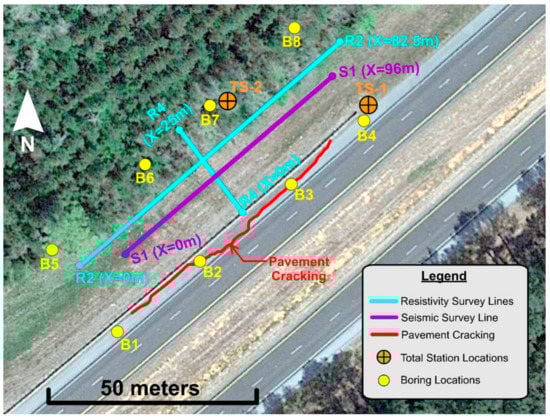
Figure 1.
Site map with locations of resistivity lines, seismic survey line, pavement cracking, total station, and borings.
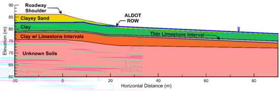
Figure 2.
Simplified site model to be used in slope stability analyses as estimated from integrated site characterization for analysis purposes.
A slow-moving landslide is located along the southbound shoulder within the roadway embankment. Persistent cracking has occurred along the southbound shoulder of the roadway over a length of approximately 63 m, which likely represents the head scarp of the landslide. The location of the landslide toe has not been observed but is thought to be beyond the Alabama Department of Transportation (ALDOT) right of way (ROW) that is about 25 m northwest of the guardrail along the southbound shoulder (roughly along the line connecting borings B5 to B8). While the location of pavement cracking is well defined, the timing of initial movement is uncertain. ALDOT personnel indicate that pavement cracking at the site has been observed as early as 2007. Google Earth images of this location show cracking as far back as 1998, and older Google Earth images make it difficult to determine the presence of cracking due to poor image resolution. It is possible that the initial failure occurred during or after the initial construction of the embankment, which was likely completed in the 1960s or early 1970s. The soils in this area are similar to Yazoo Clay in Mississippi, which has a history of low strengths and stability problems [34,35].
2.1. Characterization Tools
Investigations at this site initially consisted of borings and soil index testing (i.e., Atterberg limits) performed by ALDOT in December 2020. Additional geophysical (e.g., ERI and MASW) and lab testing (e.g., ring shear and index testing) were performed for this study. Unfortunately, no instrumentation is available at the site, so the only comparisons between the analyses and the observations are in terms of the crack locations. CPT and VST are unable to be performed at this site due to thin limestone intervals in the clay, which interfere with the penetration and operation of these tests. Figure 1 shows a map of the site and contains locations of pavement cracking, resistivity lines, seismic line, total station, and borings.
2.1.1. Total Station
Total station data are used to identify the locations of important features and estimate topography along the geophysical survey lines. Total station surveys are performed using a Topcon GTS-230W electronic total station. Total station data are primarily used in this study to estimate topography along each geophysical survey line. The locations of landmarks and boreholes are also surveyed with the total station to create a detailed site map.
2.1.2. Drilling and SPT
Drilling and SPT testing at this site were performed by ALDOT in December 2020. Borings were drilled using a CME 550X ATV rig, a CME 850X track mounted rig, and a CME 45 ATV rig. Hollow stem augers with inner diameters of 5.7 cm were used for these borings. Each rig was also equipped with a 623 N automatic hammer that was used to perform SPT testing. A total of 8 borings were drilled (Figure 1) at the site. The borings near the roadway shoulder (B1, B2, B3, and B4) were each drilled to a depth of 10.7 m. The borings performed lower on the slope (B5, B6, B7, and B8) were each drilled to a depth of 7.6 m. The water table was observed near the top of the clay layer in borings B5, B6, and B7. Water table information was not reported for the other borings. SPT testing was also performed in each boring at intervals of 46 cm in the upper 2 m and at intervals of 1.5 m below this depth. Recovered samples were tested to determine the Atterberg limits for clayey soils and used to create remolded specimens for the ring shear tests.
2.1.3. Electrical Resistivity Imaging (ERI)
Two electrical resistivity surveys were performed on 13 April 2021 (R2) and 26 May 2021 (R4). A summary of the resistivity surveys performed including date performed, number of electrodes used, electrode spacing, and line length are shown in Table 1. All surveys are performed with a commercial 8-channel SuperSting system from Advanced Geosciences Incorporated. All surveys utilize both dipole–dipole and strong gradient arrays. Inversion of the measured resistivity data is performed using the commercial software EarthImager 2D to estimate 2D pseudo-sections of subsurface resistivity distribution. The terrain along each survey line is incorporated into the inversions as estimated using a total station. The strong gradient and dipole–dipole data are inverted jointly for each survey.

Table 1.
Summary of geophysical survey parameters for both electrical resistivity (R2 and R4) and seismic (S1) surveys.
2.1.4. Seismic Testing
Seismic data were collected on 13 April 2021. A set of 48 R.T. Clark and Geostuff 4.5-Hertz geophones spaced at 2 m and a Geometrics Geode seismograms recorder are used to collect the seismic data. A geophone spacing of 2 m is used for a total line length of 94 m. Active surveys are performed using a 45 Newton sledgehammer with a sampling frequency of 2000 Hz. Passive data are also collected at a sampling frequency of 250 Hz. The seismic data are processed using the multichannel analysis of surface waves (MASW) technique. Dispersion curves are created and combined for the passive and active data. An inversion procedure is then performed to determine a one-dimensional velocity model within the desired threshold for least squares fit. The open-source software Geopsy [36,37,38] is used to select dispersion curves and perform inversions.
2.1.5. Strength Testing
Remolded clay specimens from borings B6 and B7 from depths of 1.37 m to 1.83 m are tested in a Bromhead ring shear apparatus. A specimen from boring B7 from depths of 4.12 m to 4.57 m is also tested. Kiernan presented results from multiple samples tested at the site, but this study will only consider the critical (lowest-strength) sample (B6 at a depth of 1.37 to 1.83 m). The ring shear tests are used to determine the fully softened drained strength (τfss) and the residual drained strength (τres) of the clay at the landslide site. Atterberg limits of each specimen are also measured with liquid limits ranging from 102% to 118% and plastic limits ranging from 42% to 53%.
The ring shear tests for this study are performed by reconstituting the clay specimens first to a desired water content (75%) and allowing them to rehydrate for 24 h. The clay specimens are then placed in the ring shear container and pre-consolidated to 4.6 kPa. This water content is lower than recommended by ASTM D7608 [15], which recommends preparing samples at the liquid limit. For the soils in this study, samples prepared at the liquid limit were too wet to consolidate without extruding significant material around the porous stone. Samples were iteratively prepared at lower water contents until identifying the highest water content that could be reliably used for all stress levels. Previous work by Castellanos [39] has shown that the fully softened strength is not significantly affected by the remolding water content for tests with consolidation stresses above 24 kPa. A single test was performed for this study at a water content of 98% and a consolidation stress of 22 kPa, and the fully softened strength was unaffected (Figure 3) as expected. Following the pre-consolidation stage, clay specimens are then consolidated to the desired stress levels. Vertical displacements versus time are measured during consolidation to determine appropriate shearing rates for the ring shear test according to ASTM D7608 [15] and ASTM 6467 [16]. The clay specimens are then sheared to determine the fully softened drained strength and residual drained strength envelope for each sample location. Additional details on the procedures and equipment used for this study were discussed by Xuan et al. [19].
ALDOT engineers previously performed consolidated undrained (CU) triaxial tests on undisturbed samples collected using Shelby tubes in boring B5 from depths of 1.52 m to 2.13 m. These tests were performed prior to the current study but were performed in general accordance with ASTM D4767. The first test was performed at an effective consolidation stress of 56 kPa, and the peak deviator stress was 43.8 kPa. The second test was performed at an effective consolidation stress of 164 kPa, and the peak deviator stress was 65.9 kPa. These results correspond to peak undrained shear strength ratios (su,pk/σ′v) of 0.39 and 0.20, respectively. The lower value is consistent with normally consolidated conditions, while the higher value may indicate some light overconsolidation, as would be expected in an area with a fluctuating water table. The clays in this region were deposited in a shallow marine environment, and there is no history of glaciation or other significant erosion that would be expected to produce heavily overconsolidated soils. The normally consolidated condition is more conservative and will be considered in this study to evaluate the possibility of an undrained failure.

Figure 3.
Ring shear results for both fully softened and residual strengths from samples tested at normal stresses between 22 and 125 kPa. The test results are compared with correlations from Stark [40], Castellanos et al. [41], and Mesri and Shahien [42].
Figure 3.
Ring shear results for both fully softened and residual strengths from samples tested at normal stresses between 22 and 125 kPa. The test results are compared with correlations from Stark [40], Castellanos et al. [41], and Mesri and Shahien [42].

2.2. Slope Stability Analyses
Slope stability analyses for this site are performed using both LEM and SRM. LEM analyses are performed using the commercial software SLIDE 2 [43]. Factors of safety for both circular and noncircular failure surfaces are determined with Spencer’s Method. The critical circular surfaces are found using a grid search, and critical noncircular surfaces are found using an iterative Cuckoo search. Both linear and nonlinear strength envelopes are considered for the drained strengths for LEM, while the undrained strengths are modeled using a strength ratio. SRM analyses are performed using FLAC V8.0 [44]. Undrained shear strengths (su,pk) are represented using the Mohr–Coulomb constitutive model. The cohesion value in each zone is set to the appropriate value of su,pk by multiplying the selected peak undrained shear strength ratio (su,pk/σ′v) by the vertical effective stress in the zone, and the friction angle (ϕ) is set to zero. Fully softened and residual strengths are represented using the MHB constitutive model to account for the nonlinear strength envelope of the clay. MHB parameters are calibrated to the measured strength envelopes using single element consolidated drained triaxial drivers (CDTX) in FLAC V8.0.
3. Results
3.1. Integrated Characterization
Site stratigraphy is determined using information from the drilling explorations, index tests, electrical resistivity imaging, and seismic testing (Figure 4 and Figure 5). The results of each of these tests are used to inform each other and to arrive at an integrated interpretation of the site stratigraphy and properties. Boring logs show 1 m to 4 m of clayey sands at the surface underlain by fat and lean clays with some elastic silts in borings B2 and B8. Thin intervals of limestone are also reported in the clay layers. A 20 cm (8″) thick limestone interval was encountered near boring B6 at a depth of 3.2 m (10.5′). Borings indicate the limestone interval to be a bit deeper for the borings on the roadway shoulder. The slide plane location shown in Figure 4 and Figure 5 is estimated by ALDOT personnel based on site observations and boring information. Geophysical testing and slope stability analyses are used to confirm the location of the slide plane in this study.
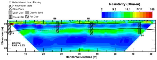
Figure 4.
Inverted resistivity profile for line R2 with boring information and estimated slide plane location.
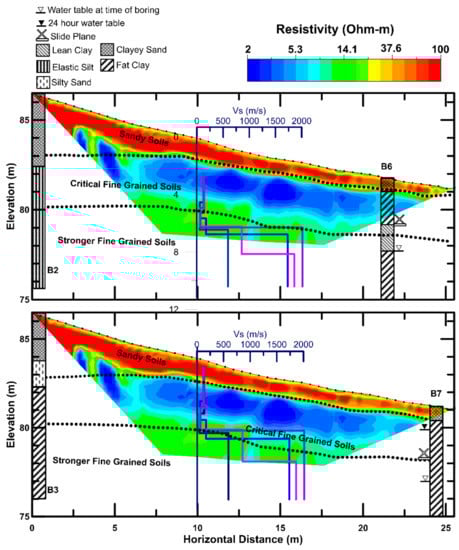
Figure 5.
Inverted resistivity profile for line R2 compared to borings B2/B3 and B6/B7 with shear wave velocity (Vs) profile from MASW line S1, boring information, and estimated slide plane location. (Note: the different seismic profiles shown in blue, dark blue, purple, and pink represent different dispersion curves selected for inversion of the measured MASW data).
The resistivity results in Figure 4 were collected near B6 and B7 (R2) and show a high-resistivity layer (14 to 100 ohm-m) near the surface (above 80 m) that correspond to the clayey sand layer encountered in the borings. A lower-resistivity layer (<5 ohm-m) is shown between elevations of 76 m to 80 m that corresponds to the upper portion of the fat clay and lean clay (B6) encountered in the borings. Liquid limits tend to be higher in this low-resistivity layer (100% to 135%) than the deeper moderate-resistivity layer (40% to 100%). Resistivity of soils is primarily based on mineral content, porosity, and water content (e.g., [4]). Soils with higher liquid limits tend to have lower resistivity (e.g., [45]). The slide plane is therefore estimated to exist in this low-resistivity layer with high liquid limits. A zone of intermediate resistivity (10 to 25 ohm-m) exists between elevations of 73 and 76 m. This zone corresponds to fat clay and elastics silts from the borings and has slightly lower liquid limits. A deeper low-resistivity zone (<5 ohm-m) also exists below an elevation of about 73 m. This layer exists below the bottom of the borings, so estimating the soil type is uncertain, but it is likely saturated limestone or marl based on the site geology. This layer is far below the expected failure planes, so it is not expected to influence the analyses in this study.
The results shown in Figure 5 are for the downslope resistivity line (R4). The resistivity line is placed between borings B2 and B6 and borings B3 and B7. The results are therefore compared to each respective set of borings and compare well with the results of Figure 4. The resistivity of the upper meter of soil is significantly higher in line R4 than R2, which is attributed to the ground being damp from recent rain during the survey of R2 and dry after over a week without rain during R4. A high-resistivity layer (>50 ohm-m) is shown near the surface. This high-resistivity layer is about 1 m thick near borings B6 and B7 and becomes thicker near the roadway shoulder. A low-resistivity layer (2 to 10 ohm-m) exists beneath the clayey sand layer and is about 2.5 m thick. This low-resistivity layer generally corresponds to fat clay from the borings B3, B6, and B7. A zone of alternating low and high resistivity can be seen in Figure 5 at horizontal distances of 2.5 m to 5 m and elevations of 82 m to 85 m. This alternating pattern of resistivity values may be due to numerical artifacts associated with the inversion attempting to fit the measured data in that area. It is also possible that preferential infiltration along cracks and shear zones allows moisture to concentrate in the lower-resistivity zones observed in this location. Either way, the results in this area should be interpreted with caution. A layer of intermediate resistivity (10 to 25 ohm-m) exists beneath the low-resistivity layer. A thin limestone layer is also encountered at a depth corresponding to the top of the intermediate-resistivity layer near boring B6, and limestone intervals are also reported in this region in the other borings. The lower LL values observed at these depths suggest these soils may have lower clay contents or lower water contents resulting in higher resistivity (e.g., [45]). The presence of limestone observed in this region may also contribute to an increase in resistivity.
Figure 5 also contains the shear wave velocity profiles obtained from the MASW survey. The different velocity profiles shown in Figure 5 correspond to different picks for the combined active and passive dispersion curves. The upper 2 m of the velocity profile is not included as data shallower than the geophone spacing of 2 m used for this survey may be unreliable [46]. The velocity profiles for the different dispersion curve picks are in general agreement with each other at depths shallower than 5 m. The seismic results show a relatively low-velocity (130 m/s) zone between 2 m to 4 m depth which corresponds to the upper clay layer identified in the borings. The velocity decreases to 60 m/s near the bottom of the low-resistivity layer which may indicate the location of the slide plane. The velocity then increases to values ranging from 600 m/s to 2000 m/s at greater depths depending on the dispersion curve pick. These results suggest the inversion is poorly constrained at greater depths. The higher range of the measured velocities is consistent with shear wave velocities of limestone measured in Alabama [47], and the lower range is consistent with reported values for Oligocene marl [48] as expected based on geology at the site. The shear wave velocity results generally agree with the resistivity results, but the velocity layer transitions occur at slightly greater depths than the resistivity layer transitions.
A simplified estimate of site stratigraphy to be used for analysis purposes is shown in Figure 2. The horizontal location of 0 m in Figure 2 is set to the location of the crest of the slope. Topography of the slope is estimated using total station measurements. This site model is developed by comparing the results of the geophysical and geotechnical explorations. More credibility is given to the data in borings B2 and B3 due to uncertainty in the resistivity profile at horizontal distances less than 5 m from the start of the line. A clayey sand layer is included near the surface which becomes thicker near the roadway shoulder. A clay layer is located beneath this sand layer which is about 2.5 m thick and represents soil within the suspected failure mass. The resistivity of this clay layer is lower than the surrounding soils which is consistent with resistivity results for landslides reported by Perrone et al. [5]. The top of the clay layer is interpreted from borings B2 and B3. Relatively low shear wave velocities are also reported in this clay layer. A thin limestone layer is located about 2.7 m below the top of the clay surface which is consistent with the location of the limestone layer encountered near B6 and the depth of the interbedded clay and limestone from the other borings. A significant increase in shear wave velocity is also observed near the expected location of the limestone interval, and the presence of limestone is expected to increase the resistivity and shear wave velocity.
3.2. Soil Properties
Soil properties for each of the soil layers considered in the analyses (Figure 2) are listed in Table 2. Shear wave velocities are used to calculate elastic moduli for the SRM analyses and are based on the MASW results (Figure 5). No measurements were taken on the limestone, and so the properties of this layer are based on published literature [49,50,51]. None of the failure surfaces intersect this layer, so the results would not be affected by reasonable variations in these properties. Similarly, properties of the layers below the limestone have no effect on the results and are not considered in the analyses. Properties of the clayey sand (unit weight and drained friction angle) were estimated using SPT-based correlations provided by Bowles [52] and Mayne and Kulhawy [53].
Table 2.
Properties of the various layers used for the slope stability analyses.
The properties of the clay layer are based on index and shear strength tests, including drained ring shear tests. The fully softened shear strength (τfss) is defined as the peak drained shear strength of this reconstituted specimen loaded under normally consolidated condition, while the residual strength is the ultimate strength reached after large displacements. Kiernan [54] presented results from multiple samples tested at the site, but this study will only consider the critical (lowest-strength) sample (B6 at a depth of 1.37 to 1.83 m). Ring shear tests are performed at normal effective stresses (σ′n) between 25 and 250 kPa to examine curvature of the strength envelope (Figure 6). Both the fully softened (Figure 6a) and residual (Figure 6b) strength envelopes show significant curvature with lower secant friction angles at higher stresses. A power curve of the form is therefore fit to the ring shear data (Table 2). The coefficient of determination (R2) for each is 0.99. These power curves are used directly in the LEM analyses and are used to calibrate the MHB constitutive model for SRM analyses.
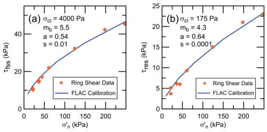
Figure 6.
Ring shear data from B6 (1.37 to 1.83 m) and MHB calibration curves to be used in SRM analyses for (a) fully softened and (b) residual shear strengths. Note: the vertical axis limits are different on each plot and are skewed with respect to the horizontal axis.
Figure 3 compares the results of the ring shear tests with correlations for both fully softened and residual strengths published by previous studies [40,41,42]. These comparisons show that the results from the current study are very consistent with these previous correlations for stress levels less than 60 kPa. The majority of the slices in the slope stability analysis have effective normal stresses between 20 and 50 kPa, which indicates that similar stability results would be obtained when using either the test data from this study or the correlations. There is a larger discrepancy between the measured results for fully softened strength at high stresses (greater than 100 kPa) and those suggested by the correlations. The secant friction angles at these high stresses are lower than would be predicted from the correlations for soils with similar Atterberg limits but are consistent with measured results for higher-plasticity soils. The reason for this discrepancy at higher stresses is unknown and needs further study but does not affect the results of these stability analyses.
Peak undrained strength (su,pk) results were measured by ALDOT using CU triaxial tests, but given the limited number of tests, published correlations are also used to estimate the undrained peak strength ratios (su,pk/σ′v). Mesri [55] suggested su,pk/σ′v is equal to 0.22 for normally consolidated clays, while Jamiliokowski et al. [56] suggested a range from 0.19 to 0.23. A baseline su,pk/σ′v value of 0.21 is selected for the analyses based on these correlations and the CU results for the higher stress level. Kiernan [54] also examined 0.19 and 0.23 to account for uncertainty of normally consolidated strength and overconsolidation ratio (OCR), but there is no evidence to believe the soils in the critical zone are overconsolidated based on blow counts (N = 4 to 7) and site geology. The LEM analyses in this study utilize a vertical stress ratio to represent undrained shear strength. SRM analyses utilize a Mohr–Coulomb model with a friction angle of zero and cohesion set to a value of su,pk/σ′v multiplied by the initial value of vertical effective stress in each zone.
3.3. Model Calibration
SRM analyses are performed using FLAC V8.0 which does not include a power curve option for representing the nonlinear strength envelopes observed in the ring shear data. The modified Hoek–Brown (MHB) constitutive model is therefore used to represent drained strengths in SRM analyses due to its ability to represent nonlinear shear strength behavior [27]. Calibration of the MHB parameters to fully softened and residual drained strength is performed using a single element consolidated drained triaxial (CDTX) driver in FLAC. The MHB parameters σci, mb, a, and s are iteratively adjusted to fit the ring shear data at σ′n values up to 250 kPa. While these parameters have physical meaning for rock testing, they are simply used as calibration parameters when applying the model to soil. Results from the model calibration are compared to the ring shear results in Figure 6.
3.4. Slope Stability Results
Slope stability analyses are performed to investigate probable failure mechanisms at the landslide site and to compare results using LEM and SRM. As previously discussed, the slope has been intermittently moving for decades with cracks and settlement routinely appearing in the shoulder after large rain events. Analyses using fully softened drained shear strength in the clay are investigated first to determine if the initial failure could have occurred under drained conditions. Peak undrained shear strengths are examined next to investigate the possibility of an initial undrained failure. Residual drained strengths are then examined to estimate stability of the slope on a pre-existing shear surface. The effect of potential strength gain and changes in water table elevation are also examined. Kiernan [54] also examined the effect of element height on the SRM results. The baseline (medium) mesh in this manuscript uses element heights of 0.75 m, while Kiernan [54] also examined a coarse mesh with element heights of 1.5 m and a fine mesh with element heights of 0.25 m. The fine and medium mesh produced the same FS value indicating that the baseline (medium) mesh used in this study is sufficiently discretized, while the coarse mesh produced a 25% higher FS value. This highlights the importance of considering mesh size effects when performing SRM analyses.
3.4.1. Analyses for an Initial Drained Failure
LEM analyses are first performed using fully softened drained strength parameters estimated from ring shear testing (Table 2). Previous research has shown the fully softened strength to be appropriate for analyzing first-time failures in high-plasticity clay soils (e.g., [1,17]). FS values range from 1.57 for the circular failure surfaces to 1.49 for the noncircular failure surfaces (Table 3). Failure planes using circular and noncircular surfaces from LEM analyses are shown in Figure 7. The noncircular surface reaches the ground surface behind the location where cracking is observed along the shoulder and follows the limestone layer closely across the central portion of the embankment. The toe of the failure surface is located near the ALDOT ROW boundary. The circular surface is generally similar to the noncircular surface for the analyses using the fully softened drained strength. Both surfaces are consistent with observations, but the FS values indicate adequate stability under these conditions.
Table 3.
Factors of safety for various conditions examined in the slope stability analyses.
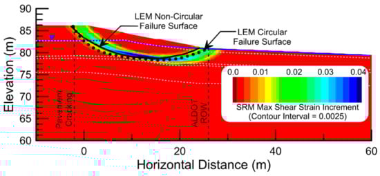
Figure 7.
Maximum shear strain interval contours (zoomed in on failure surface location) from SRM analysis using fully softened drained strengths with critical noncircular failure surface from LEM shown as solid black line and critical failure surface from LEM with circular surfaces shown by dotted black line. Locations of ALDOT ROW and observed pavement cracking are shown as dashed lines. Soil boundaries (Figure 2) are shown by dotted light grey lines.
The FS from the SRM is shown in Table 3, and shear strain contours from the SRM results are shown in Figure 7. SRM does not provide a single failure surface, but the area of highest shear strain generally corresponds to the slide plane. SRM is not constrained by the location and shape of the failure surface or assumptions regarding the inclination of interslice forces [24]. The failure surfaces from the LEM analyses closely match the areas of greatest shear strain from the SRM giving additional confidence in the use of the MHB model to represent the strength of this clay, while the factor of safety is slightly lower than the LEM results. This agreement demonstrates the accuracy of the SRM using MHB parameters to represent nonlinear strength envelopes of clays.
3.4.2. Analyses for an Initial Undrained Failure
The possibility of an undrained failure is investigated by using a vertical stress ratio equal to su,pk/σ′v for the clay layer while keeping the other properties constant. The associated FS values are shown in Table 3, and the critical failure surfaces are shown in Figure 8. FS values range from 0.97 for the circular failure surface to 0.91 for the noncircular failure surface. The higher FS values observed for the circular failure surfaces are consistent with the LEM results of the initial drained failure investigation. In addition to having a higher FS, the critical circular surface is located on the face of the slope downhill from the roadway. The shear strain contours from the SRM analysis are similar to the critical noncircular surface (Figure 8) but with a higher FS of 1.02. These results indicate that instability is possible due to undrained loading of the clay, but the mechanism of this undrained loading is not known. It is possible that an undrained failure might have occurred during initial construction of the embankment, but no information is available regarding the initial slope geometry, effective stress conditions, or any possible OCR within the clay at the time of construction. Without this information, it is not possible to accurately evaluate an undrained failure during initial construction. The factor of safety value for an undrained failure under current conditions is near 1, which indicates only minimal movement would be expected even if a failure did occur.
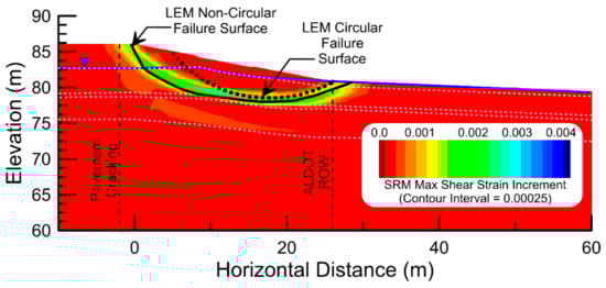
Figure 8.
Maximum shear strain interval contours (zoomed in on failure surface location) from initial peak undrained (su,pk/σ′v = 0.21) SRM analysis with critical noncircular failure surface from LEM shown as solid black line and critical failure surface from LEM with circular surfaces shown by dotted black line. Locations of ALDOT ROW and pavement cracking shown by dashed black lines. Soil layer boundaries (Figure 2) shown by dotted light grey lines.
3.4.3. Analyses for Residual Drained Strengths
The previous results show that the initial failure at this location could have been triggered by undrained loading of the clay. Once a failure surface forms, residual strengths are appropriate to examine the potential for reactivation. LEM analyses with residual strengths give an FS of 0.81 for the circular failure surface, 0.71 for the noncircular surface, and 0.76 for SRM. Failure planes for the residual strengths are similar to those shown in Figure 7 for the fully softened strengths, except the noncircular failure surface is slightly shallower due to the high strength assumed in the limestone layer. The FS values obtained for each method using drained fully softened strength parameters are significantly lower than 1 indicating that continued movement of the slope may occur on a preexisting failure plane under drained loading. However, such low FS values indicate that large movements would be expected at the site, which is not consistent with observations. It is possible that the mobilized strength at the site is between the residual and fully softened strengths due to strength gain, a fluctuating water table, or the slope may not have moved enough to fully remold the materials along the failure plane.
The effect of lowering the water table and possible strength recovery is examined using the residual strength envelope and the noncircular LEM analysis. Previous research suggests that soil within a preexisting landslide failure plane may recover strength with time (e.g., [57,58,59]). Stark and Hussain [60] examined data from previous researchers and found that clay soils may recover 10% to 40% of the residual drained shear strength over a period of 3 days to 5 months, but little movement may be required to re-mobilize the drained residual shear strength. This effect is incorporated into the current analyses by the ‘a’ parameter in the power envelope to achieve strength recovery of 20%, 30%, and 40% for vertical stresses up to 150 kPa (Figure 8 and Table 4). Even the 40% increase in strength is still significantly less than the fully softened envelope (Figure 6a), which had an ‘a’ parameter of 1.64.
Table 4.
Updated power curve parameters for strength recovery using drained residual strength ring shear results with FS values for the baseline and lowered water tables (WT).
The FS for the increased strength is shown in Table 4 for both the baseline water table (Figure 2) and a water table, which is 2 m lower than the baseline. The lower water table is meant to account for seasonal fluctuations, which may occur in tandem with a reduction in movement and subsequent strengthening. The FS increases with increasing strength and lowering of the water table, as expected. The FS is close to 1 for strength gains greater than 40% with the baseline water table or as low as 20% with the lower water table. These results suggest that slope movements may cease as the water table elevation decreases and strength is recovered on the preexisting failure plane. However, the relationship between a decreasing water table elevation and strength recovery on the failure is not well understood and requires further research.
4. Discussion and Conclusions
This study integrates geophysics with traditional geotechnical explorations, index tests, and lab testing to characterize a slow-moving landslide site in Alabama. The data from all sources are used to inform each other to build a site model for use in slope stability analyses. Geophysical results are shown to correspond well with boring information. ERI provides a continuous 2D profile, is shown to delineate the clay layer from the surrounding soil mass, and corresponds well with Atterberg limits of the fine-grained layers. MASW helps delineate lower-velocity soils in the failure mass from stiffer soils outside the soil mass and appears to identify a shear plane of lower velocity. The ERI and MASW can therefore be used to create a detailed model of the site with high confidence compared to interpolating between point data collected from the boring locations. ERI and MASW are reliable tools for estimating site stratigraphy, but interpretation required integrating these results with results from other methods. Results from traditional geotechnical explorations (i.e., borings and SPT) and index test (i.e., Atterberg limits) should be used to guide interpretation of geophysical results to arrive at an accurate estimate of site stratigraphy.
Ring shear testing is used to determine drained fully softened and residual shear strengths for clay samples collected from borings. The drained fully softened and residual strength envelopes obtained from ring shear testing are shown to be nonlinear. Both envelopes are consistent with previous correlations in the stress range of interest for this study. A power curve is used to represent the nonlinear strength envelopes in LEM, and the modified Hoek–Brown constitutive model is used to represent the nonlinear strength envelopes for SRM analyses in FLAC. FS values from LEM analyses using the power curve representation of shear strength are comparable to SRM analyses. The MHB model is therefore shown to provide a practical option for representing nonlinear strength envelopes of soils in SRM analyses.
Circular and noncircular failure surfaces are compared in LEM analyses. Circular surfaces are shown to produce higher FS values (approximately 10%) compared to noncircular surfaces. Circular surfaces produced shallower failure planes than noncircular surfaces but are generally consistent with site observations when drained fully softened and residual strength envelopes are used. The difference between circular and noncircular surfaces is most prevalent when undrained shear strength is analyzed. The undrained circular failure plane is observed to breach the ground surface on the face of the slope which is not consistent with site observations. Differences in FS values obtained using circular and noncircular surfaces are also larger in the undrained analyses. The constraint of a circular failure surface in LEM may misrepresent the critical surface for cases involving more complex failure plane geometries. The results of this study suggest, this limitation may be more significant for undrained analyses where the friction angle is zero.
The results of LEM analyses are also compared to SRM analyses. SRM produces lower-bound FS values for the initial drained failure investigation but not for the residual drained failure or peak undrained failure investigations. Itasca [44] stated that LEM should never produce a lower-bound FS compared to SRM and suggested that LEM may be unreliable in cases where LEM provides a lower-bound FS. This statement contradicts the findings in this study as well as the conclusions of Cheng et al. [61]. Noncircular LEM failure planes in this study sometimes produce slightly higher FS values compared to SRM, but the noncircular failure planes are generally consistent with the critical failure plane locations produced by SRM. The comparison of both methods illustrates that LEM and SRM are both valid methods for analyzing slope stability problems. LEM and SRM analyses should both be performed for a given case history to compare the results.
The main objective is to understand the failure mechanism for this landslide. Repeated failure along a preexisting shear plane is assumed to occur at the site due to the recurrent movements observed. The time and mechanism of the initial failure causing the preexisting shear plane are not known. FS values obtained using the fully softened drained strength envelopes indicate that initial failure likely did not occur under drained loading. FS values obtained using undrained shear strength ratios produce FS values just above or below 1 indicating that initial failure of the slope likely occurred under undrained loading. Analyses utilizing the residual drained strength envelopes produce FS values significantly lower than 1 indicating the slope to be unstable when soil on the failure plane exists at the residual state. The low FS values obtained using residual drained strengths suggest that more rapid deformations than observed in the field may be expected if the residual shear strength is sustained on the failure plane.
Clays at a residual state have been shown to recover strength with time. The effect of shear strength increase due to strength recovery on the failure plane is examined in this study using failure envelopes that produce shear strengths 20% to 40% greater than the measured residual values. Strength recovery on the failure plane is shown to significantly increase FS values, but the strength increase alone is not large enough to produce a stable slope. Lowering of the water table increased FS values significantly but did not produce a stable slope. The combined effect of strength recovery and a lowered water table is also examined and is found to produce FS values greater than 1 indicating a stable slope.
The results of slope stability analyses in this study indicate that the slope likely became unstable due to undrained loading. Continued movement of the slope observed after rain events likely occurs as the water table rises and the mobilized drained shear strength on the failure plane is somewhere between the residual and fully softened values. The combined effect of the WT elevation decreasing after rain events and strength recovery along the failure plane produces a stable slope during dry periods when movement is not observed. The relationship between strength recovery and changes in water table elevation is not well understood and remains a topic for future research.
Author Contributions
Conceptualization, J.M. and J.B.A.; methodology, J.M. and J.B.A.; investigation, M.K. and M.X.; resources, J.M. and J.B.A.; writing—original draft preparation, M.K. and J.M.; writing—review and editing, M.X. and J.B.A.; visualization, M.K.; supervision and project administration, J.M.; funding acquisition, J.M. and J.B.A. All authors have read and agreed to the published version of the manuscript.
Funding
This research was funded by the Alabama Department of Transportation, grant number 930-988, and the Auburn University Highway Research Center.
Data Availability Statement
The data used in this study are presented within the body of the article and may also be obtained by contacting the corresponding author.
Acknowledgments
We appreciate the support and assistance provided by Kaye Chancellor Davis and Brannon McDonald with the Alabama Department of Transportation throughout this project. We are also grateful to Patricia Carcamo for processing the seismic data and to Chukwuma Okafor, Ashton Babb, Tyler Belk, and Frank Russell for assisting with the field work.
Conflicts of Interest
The authors declare no conflict of interest.
References
- Wright, S.G.; Zornberg, J.G.; Aguettant, J.E. The Fully Softened Shear Strength of High Plasticity Clays; Center for Transportation Research, University of Texas at Austin: Austin, TX, USA, 2007. [Google Scholar]
- Knights, M.J.; Montgomery, J.; Carcamo, P.S. Development of a Slope Failure Database for Alabama Highways. Bull. Eng. Geol. Environ. 2020, 79, 423–438. [Google Scholar] [CrossRef]
- Montgomery, J.; Kiernan, M.; Jackson, D.; McDonald, B. Integrating Surface-Based Geophysics into Landslide Investigations along Highways. In Proceedings of the Geo-Congress 2022, American Society of Civil Engineers, Charlotte, NC, USA, 17 March 2022; pp. 180–191. [Google Scholar] [CrossRef]
- Loke, M.H. Tutorial: 2-D and 3-D Electrical Imaging Surveys. Geotomo Software. 2021. Available online: https://www.researchgate.net/publication/264739285_Tutorial_2-D_and_3-D_Electrical_Imaging_Surveys (accessed on 21 September 2022).
- Perrone, A.; Lapenna, V.; Piscitelli, S. Electrical Resistivity Tomography Technique for Landslide Investigation: A Review. Earth-Sci. Rev. 2014, 135, 65–82. [Google Scholar] [CrossRef]
- Jongmans, D.; Garambois, S. Geophysical investigation of landslides: A Review. Bull. Soc. Géol. Fr. 2007, 178, 101–112. [Google Scholar] [CrossRef]
- Chae, B.-G.; Park, H.-J.; Catani, F.; Simoni, A.; Berti, M. Landslide Prediction, Monitoring and Early Warning: A Concise Review of State-of-the-Art. Geosci J. 2017, 21, 1033–1070. [Google Scholar] [CrossRef]
- Embankments, Dams, and Slopes Technical Committee; Stark, T.D.; Oommen, T.; Ning, Z.; Bouali, E.H.; Arasa, N.D.; Gregory, P.; Hughes, K.S.; Leshchinsky, B.; Praeg, R.; et al. Remote Sensing for Monitoring Embankments, Dams, and Slopes: Recent Advances; American Society of Civil Engineers: Reston, VA, USA, 2021; ISBN 978-0-7844-1572-6. [Google Scholar]
- Travelletti, J.; Malet, J.-P. Characterization of the 3D Geometry of Flow-like Landslides: A Methodology Based on the Integration of Heterogeneous Multi-Source Data. Eng. Geol. 2012, 128, 30–48. [Google Scholar] [CrossRef]
- Bunn, M.; Leshchinsky, B.; Olsen, M.J. Geologic Trends in Shear Strength Properties Inferred through Three-Dimensional Back Analysis of Landslide Inventories. J. Geophys. Res. Earth Surf. 2020, 125, e2019JF005461. [Google Scholar] [CrossRef]
- Donohue, S.; Long, M.; O’Connor, P.; Helle, T.E.; Pfaffhuber, A.; Rømoen, M. Geophysical Mapping of Quick Clay—A Case Study from Smørgrav, Norway. In Proceedings of the Near Surface 2009—15th EAGE European Meeting of Environmental and Engineering Geophysics, Dublin, Ireland, 7–9 September 2009; European Association of Geoscientists & Engineers: Dublin, Ireland, 2009. [Google Scholar] [CrossRef]
- Jongmans, D.; Bièvre, G.; Renalier, F.; Schwartz, S.; Beaurez, N.; Orengo, Y. Geophysical Investigation of a Large Landslide in Glaciolacustrine Clays in the Trièves Area (French Alps). Eng. Geol. 2009, 109, 45–56. [Google Scholar] [CrossRef]
- Huntley, D.; Bobrowsky, P.; Hendry, M.; Macciotta, R.; Best, M. Multi-Technique Geophysical Investigation of a Very Slow-Moving Landslide near Ashcroft, British Columbia, Canada. JEEG 2019, 24, 87–110. [Google Scholar] [CrossRef]
- Stark, T.D.; Vettel, J.J. Bromhead Ring Shear Test. Procedure. Geotech. Test. J. 1992, 15, 24–32. [Google Scholar] [CrossRef]
- ASTM D7608-18e1; Standard Test Method for Torsional Ring Shear Test to Measure Drained Fully Softened Shear Strength and Stress Dependent Strength Envelope of Fine-Grained Soils. ASTM International: West Conshohocken, PA, USA, 2018. [CrossRef]
- ASTM D6467-13e; Standard Test Method for Torsional Ring Shear Test to Determine Drained Residual Shear Strength of Fine-Grained Soils. ASTM International: West Conshohocken, PA, USA, 2018. [CrossRef]
- Skempton, A.W. First-time slides in over-consolidated clays. Géotechnique 1970, 20, 320–324. [Google Scholar] [CrossRef]
- Stark, T.D.; Eid, H.T. Slope Stability Analyses in Stiff Fissured Clays. J. Geotech. Geoenviron. Eng. 1997, 123, 335–343. [Google Scholar] [CrossRef]
- Xuan, M.; Montgomery, J.; Anderson, J.B. Examining the Effects of Suction and Nonlinear Strength Envelopes on the Stability of a High Plasticity Clay Slope. Geosciences 2021, 11, 449. [Google Scholar] [CrossRef]
- Baker, R. Nonlinear Mohr Envelopes Based on Triaxial Data. J. Geotech. Geoenviron. Eng. 2004, 130, 498–506. [Google Scholar] [CrossRef]
- Atkinson, J. Peak strength of overconsolidated clays. Géotechnique 2007, 57, 127–135. [Google Scholar] [CrossRef]
- VandenBerge, D.R.; Castellanos, B.A.; McGuire, M.P. Comparison and Use of Failure Envelope Forms for Slope Stability Analyses. Geotech. Geol. Eng. 2019, 37, 2029–2046. [Google Scholar] [CrossRef]
- Duncan, J.M.; Wright, S.G.; Brandon, T.L. Soil Strength and Slope Stability; John Wiley: Hoboken, NJ, USA, 2014. [Google Scholar]
- Dawson, E.M.; Roth, W.H.; Drescher, A. Slope Stability Analysis by Strength Reduction. Geotechnique 1999, 49, 835–840. [Google Scholar] [CrossRef]
- Perry, J. A Technique for Defining Nonlinear Shear Strength Envelopes, and Their Incorporation in a Slope Stability Method of Analysis. Q. J. Eng. Geol. Hydrogeol. 1994, 27, 231–241. [Google Scholar] [CrossRef]
- Jiang, J.-C.; Baker, R.; Yamagami, T. The Effect of Strength Envelope Nonlinearity on Slope Stability Computations. Can. Geotech. J. 2003, 40, 308–325. [Google Scholar] [CrossRef]
- VandenBerge, D.R.; McGuire, M.P. Practical Use of Modified Hoek–Brown Criterion for Soil Slope Stability Analysis. Geotech. Geol. Eng. 2019, 37, 5441–5455. [Google Scholar] [CrossRef]
- Sun, C.; Chai, J.; Luo, T.; Xu, Z.; Chen, X.; Qin, Y.; Ma, B. Nonlinear Shear-Strength Reduction Technique for Stability Analysis of Uniform Cohesive Slopes with a General Nonlinear Failure Criterion. Int. J. Geomech. 2021, 21, 06020033. [Google Scholar] [CrossRef]
- Hoek, E.; Carranza-Torres, C.; Corkum, B. Hoek-Brown Failure Criterion—2002 Edition. In Proceedings of the 5th North American Rock Mechanics and 17th Tunnelling Association of Canada Conference (NARMS-TAC), Toronto, ON, Canada, 7–10 July 2002; pp. 267–273. [Google Scholar]
- Sun, C.; Chai, J.; Luo, T.; Xu, Z.; Qin, Y.; Yuan, X.; Ma, B. Stability Charts for Pseudostatic Stability Analysis of Rock Slopes Using the Nonlinear Hoek–Brown Strength Reduction Technique. Adv. Civ. Eng. 2020, 2020, 8841090. [Google Scholar] [CrossRef]
- Sun, C.; Chai, J.; Xu, Z.; Qin, Y.; Chen, X. Stability Charts for Rock Mass Slopes Based on the Hoek-Brown Strength Reduction Technique. Eng. Geol. 2016, 214, 94–106. [Google Scholar] [CrossRef]
- Szabo, M.; Osborne, W.; Copeland, C., Jr.; Neathery, T. Geologic Map of Alabama (1:250,000): Alabama Geological Survey Special Map 220; Geological Survey of Alabama: Uscaloosa, AL, USA, 1988. [Google Scholar]
- Cook, M.; Baker, R.M.; Henderson, P.; McGregor, S.; Moss, N. Conecuh-Sepulga-Blackwater Rivers Watershed Protection Plan; Alabama Geologic Survey: Tuscaloosa, AL, USA, 2004. [Google Scholar]
- Nobahar, M.; Khan, M.S.; Stroud, M.; Amini, F.; Ivoke, J. Progressive Development of the Perched Water Zone in Highway Slopes Made of Highly Plastic Clay. Transp. Res. Rec. 2021, 2675, 715–728. [Google Scholar] [CrossRef]
- Khan, M.S.; Nobahar, M.; Stroud, M.; Ferguson, S.; Ivoke, J. Performance Evaluation of a Highway Slope on Expansive Soil in Mississippi. Int. J. Geomech. 2022, 22, 05021005. [Google Scholar] [CrossRef]
- Wathelet, M. Array Recordings of Ambient Vibrations: Surface-Wave Inversion. Ph.D. Thesis, Faculté des Sciences Appliquées, Liege University, Liege, Belgium, 2005. [Google Scholar]
- Wathelet, M. An Improved Neighborhood Algorithm: Parameter Conditions and Dynamic Scaling. Geophys. Res. Lett. 2008, 35, L09301. [Google Scholar] [CrossRef]
- Wathelet, M.; Chatelain, J.-L.; Cornou, C.; Giulio, G.D.; Guillier, B.; Ohrnberger, M.; Savvaidis, A. Geopsy: A User-Friendly Open-Source Tool Set for Ambient Vibration Processing. Seismol. Res. Lett. 2020, 91, 1878–1889. [Google Scholar] [CrossRef]
- Castellanos, B.A. Use and Measurement of Fully Softened Shear Strength. Ph.D. Thesis, Virginia Tech, Blacksburg, VA, USA, 2014. [Google Scholar]
- Stark, T.D. Spreadsheet for Drained Residual and Fully Softened Secant Friction Angles. 2022. Available online: https://tstark.net/wp-content/uploads/2012/10/Residual-FullySoftened-Correlations-2022-01-09-2022-LOCKED-Laboratory-2022.xlsx (accessed on 21 September 2022).
- Castellanos, B.A.; Ritchie, J.; Brandon, T.L. Estimating Fully Softened and Residual Shear Strength Parameters of Fine-Grained Soils; Center for Geotechnical Practice and Research, Virginia Tech: Blacksburg, VA, USA, 2021. [Google Scholar]
- Mesri, G.; Shahien, M. Residual Shear Strength Mobilized in First-Time Slope Failures. J. Geotech. Geoenviron. Eng. 2003, 129, 12–31. [Google Scholar] [CrossRef]
- Rocscience, Inc. Slide 2-2D Limit Equilibrium Analysis for Slopes, Version 9.013; Rocscience, Inc.: Toronto, ON, Canada, 2021.
- Itasca. FLAC, “Fast Lagrangian Analysis of Continua”, Version 8.0; Itasca Consulting Group: Minneapolis, MN, USA, 2016.
- Abu-Hassanein, Z.S.; Benson, C.H.; Blotz, L.R. Electrical Resistivity of Compacted Clays. J. Geotech. Eng. 1996, 122, 397–406. [Google Scholar] [CrossRef]
- Park, C.B.; Miller, R.D.; Xia, J. Multichannel Analysis of Surface Waves. Geophysics 1999, 64, 800–808. [Google Scholar] [CrossRef]
- Montgomery, J.; Jackson, D.; Kiernan, M.; Anderson, J.B. Use of Geophysical Methods for Sinkhole Exploration; ALDOT Report 930-945; Highway Research Center, Auburn University: Auburn, AL, USA, 2020. [Google Scholar]
- Mayne, P. Stress-Strain-Strength-Flow Parameters from Enhanced in-Situ Tests. In Proceedings of the International Conference on In-Situ Measurement of Soil Properties & Case Histories [In-Situ 2001], Bali, Indonesia, 21–24 May 2001; pp. 27–47. [Google Scholar]
- McVay, M.C.; Townsend, F.C.; Williams, R.C. Design of Socketed Drilled Shafts in Limestone. J. Geotech. Eng. 1992, 118, 1626–1637. [Google Scholar] [CrossRef]
- Gaviglio, P. Longitudinal Waves Propagation in a Limestone: The Relationship between Velocity and Density. Rock Mech. Rock Eng. 1989, 22, 299–306. [Google Scholar] [CrossRef]
- Yaşar, E.; Erdoğan, Y. Estimation of Rock Physicomechanical Properties Using Hardness Methods. Eng. Geol. 2004, 71, 281–288. [Google Scholar] [CrossRef]
- Bowles, J.E. Foundation Analysis and Design, 5th ed.; McGraw-Hill: Singapore, 1996. [Google Scholar]
- Kulhawy, F.H.; Mayne, P.W. Manual on Estimating Soil Properties for Foundation Design; Electric Power Research Inst.: Palo Alto, CA, USA; Cornell Univ.: Ithaca, NY, USA, 1990. [Google Scholar]
- Kiernan, M. Site Characterization and Modeling Considerations for Slopes Involving Fine Grained Strain-Softening Soils. Ph.D. Thesis, Auburn University, Auburn, AL, USA, 2021. [Google Scholar]
- Mesri, G. A Reevaluation of Su(Mob) = 0.22σ′p Using Laboratory Shear Tests. Can. Geotech. J. 1989, 26, 162–164. [Google Scholar] [CrossRef]
- Jamiolkowski, M.; Ladd, C.C.; Germaine, J.T.; Lancellotta, R. New Developments in Field and Laboratory Testing of Soils. In Proceedings of the 11th International Conference on Soil Mechanics and Foundation Engineering, San Francisco, CA, USA, 12–16 August 1985; pp. 57–153. [Google Scholar]
- D’Appolonia, E.; Alperstein, R.; D’Appolonia, D.J. Behavior of a Colluvial Slope. J. Soil Mech. Found. Div 1967, 93, 447–473. [Google Scholar] [CrossRef]
- Ramiah, B.K.; Purushothamaraj, P.; Tavane, N.G. Thixotropic Effects on Residual Strength of Remoulded Clays. Indian Geotech. J. 1973, 3, 189–197. [Google Scholar]
- Skempton, A.W. Residual strength of clays in landslides, folded strata and the Laboratory. Géotechnique 1985, 35, 3–18. [Google Scholar] [CrossRef]
- Stark, T.D.; Hussain, M. Shear Strength in Preexisting Landslides. J. Geotech. Geoenviron. Eng. 2010, 136, 957–962. [Google Scholar] [CrossRef]
- Cheng, Y.M.; Lansivaara, T.; Wei, W.B. Two-Dimensional Slope Stability Analysis by Limit Equilibrium and Strength Reduction Methods. Comput. Geotech. 2007, 34, 137–150. [Google Scholar] [CrossRef]


Publisher’s Note: MDPI stays neutral with regard to jurisdictional claims in published maps and institutional affiliations. |
© 2022 by the authors. Licensee MDPI, Basel, Switzerland. This article is an open access article distributed under the terms and conditions of the Creative Commons Attribution (CC BY) license (https://creativecommons.org/licenses/by/4.0/).