
Mapping Underwater Bathymetry of a Shallow River from Satellite Multispectral Imagery


Abstract
:1. Introduction
2. Methods
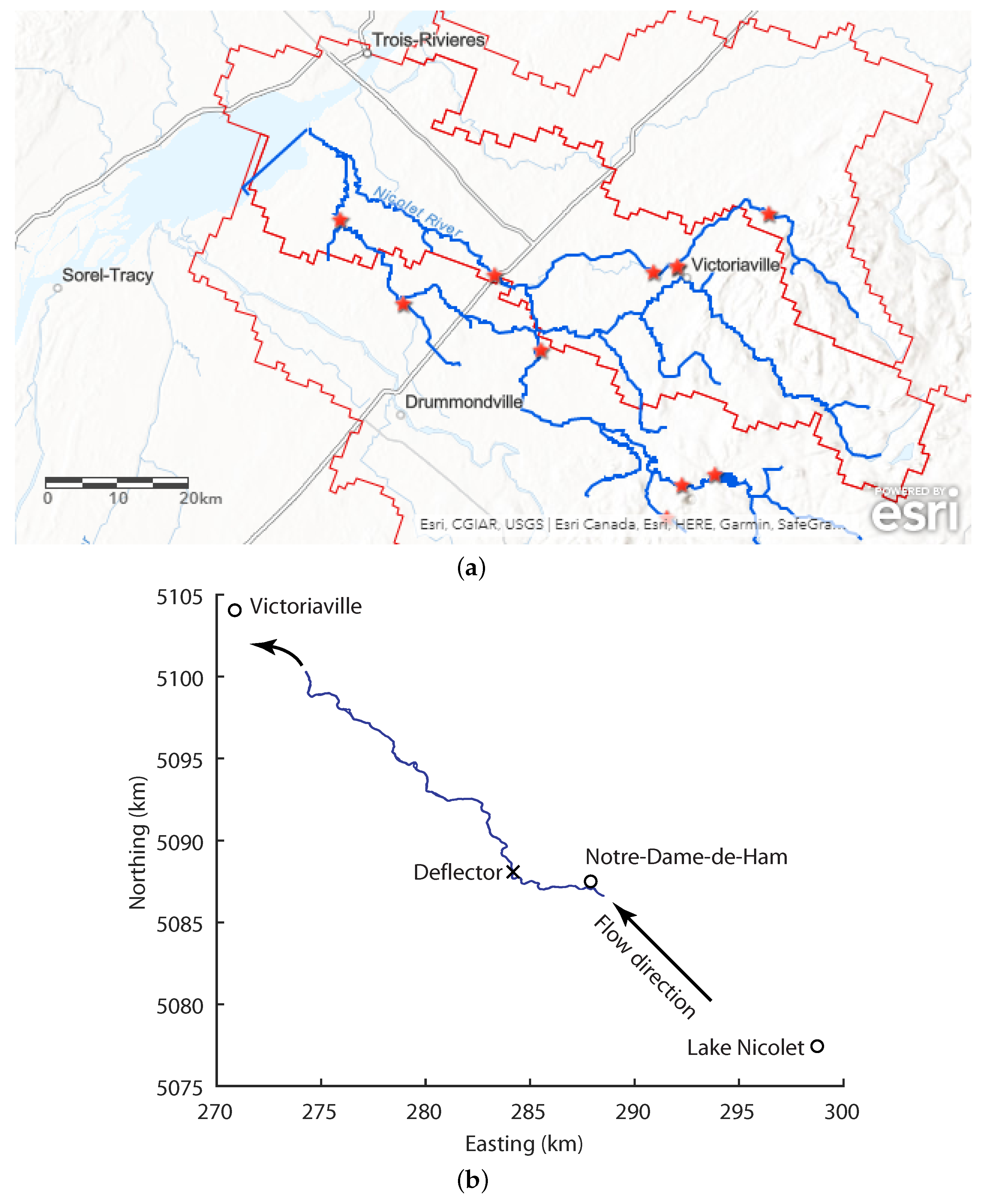
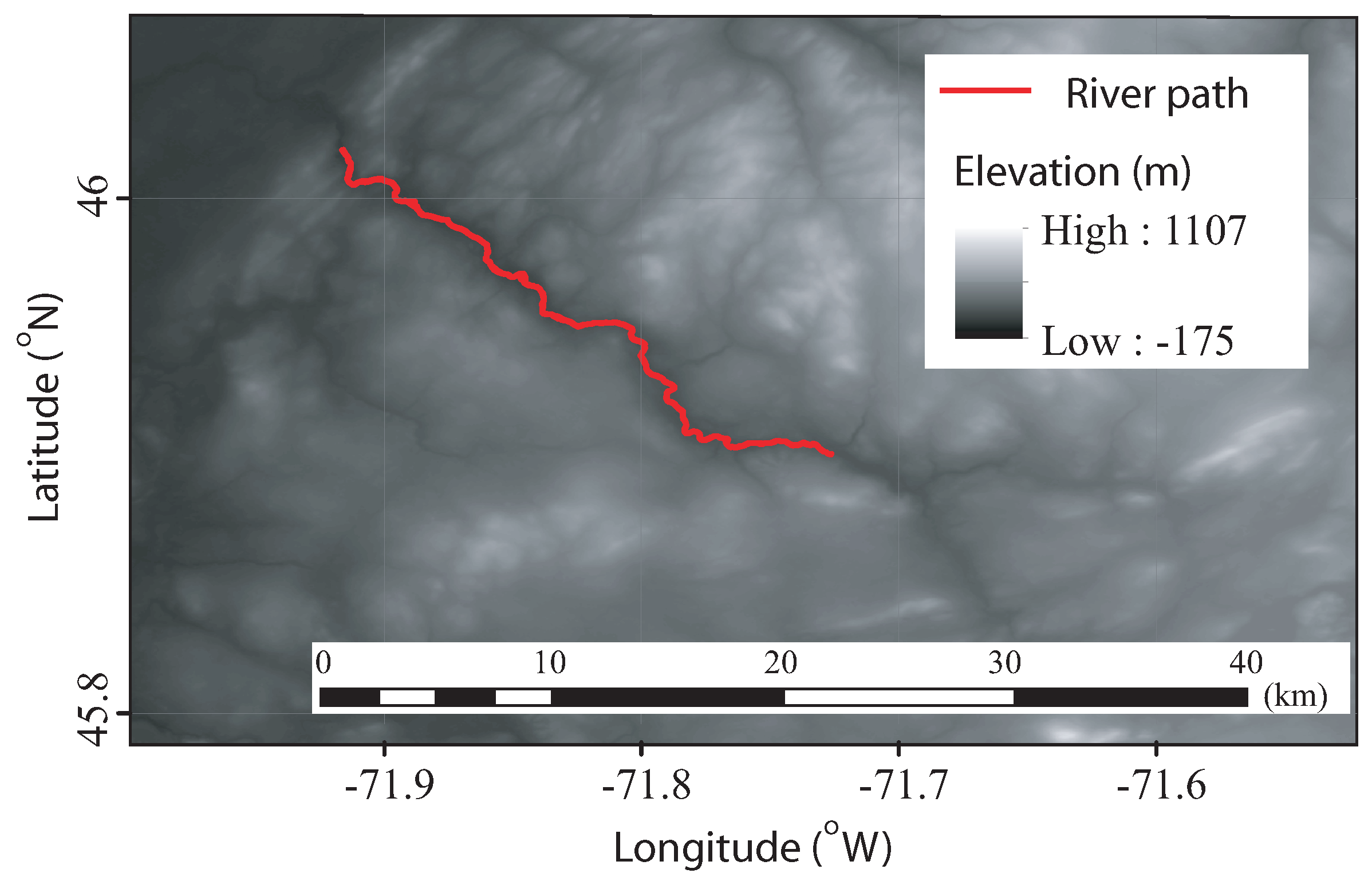
2.1. Site of Study
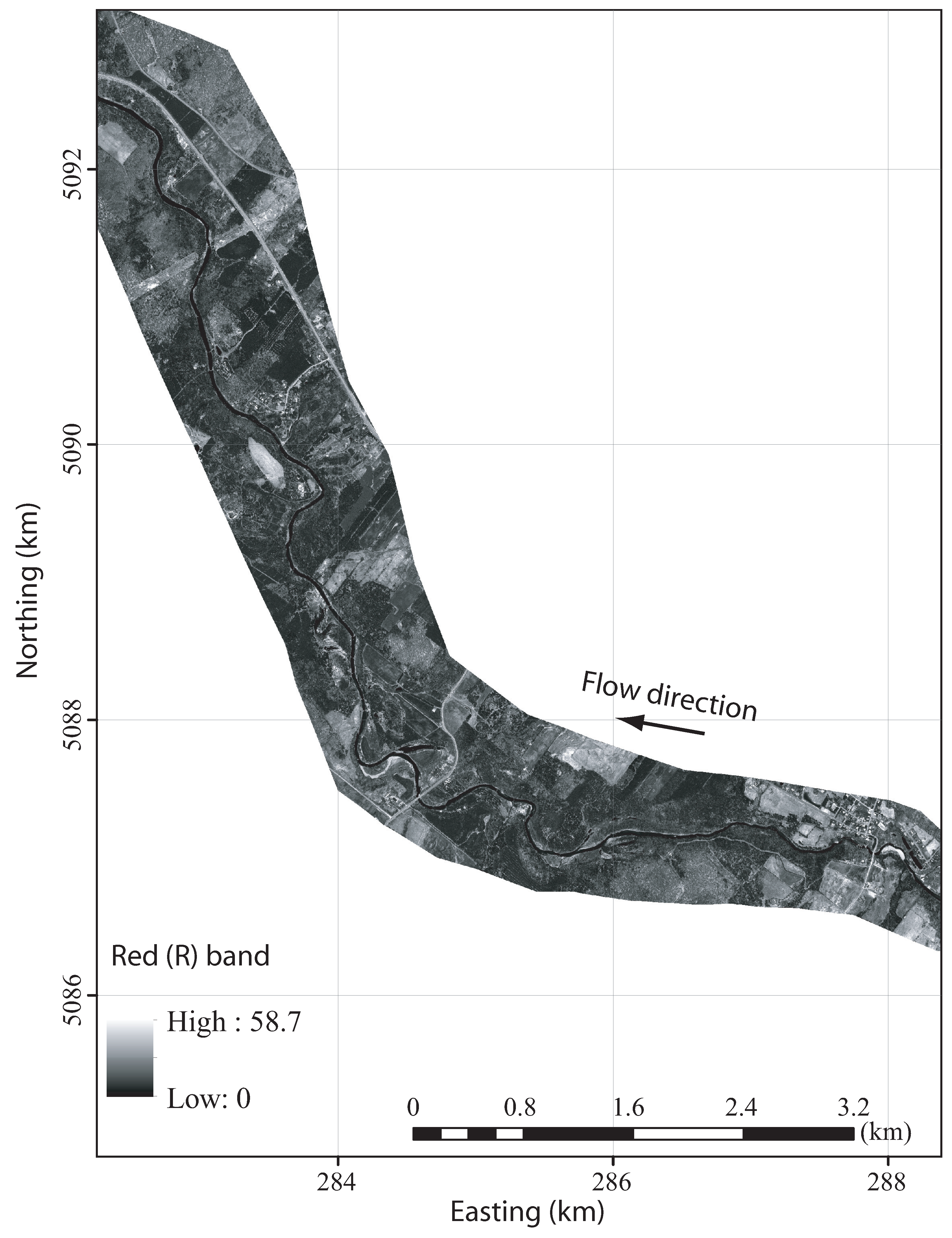
2.2. WV-3 Multispectral Image
2.3. Calculation of Top-of-Atmosphere Spectral Radiance
2.4. Calculation of TOA Reflectance
2.5. Identification of River Water Pixels
2.6. Geo-Reference of Pixels in the WV-3 Image
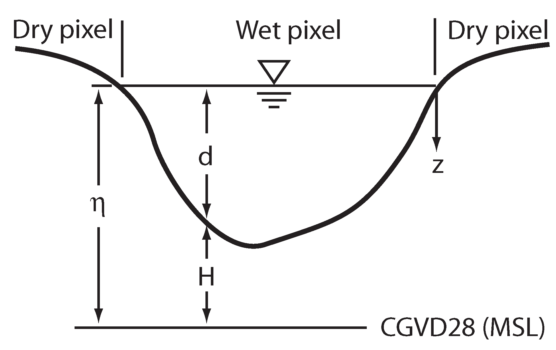
2.7. Calculation of River Flow Depth
3. Results
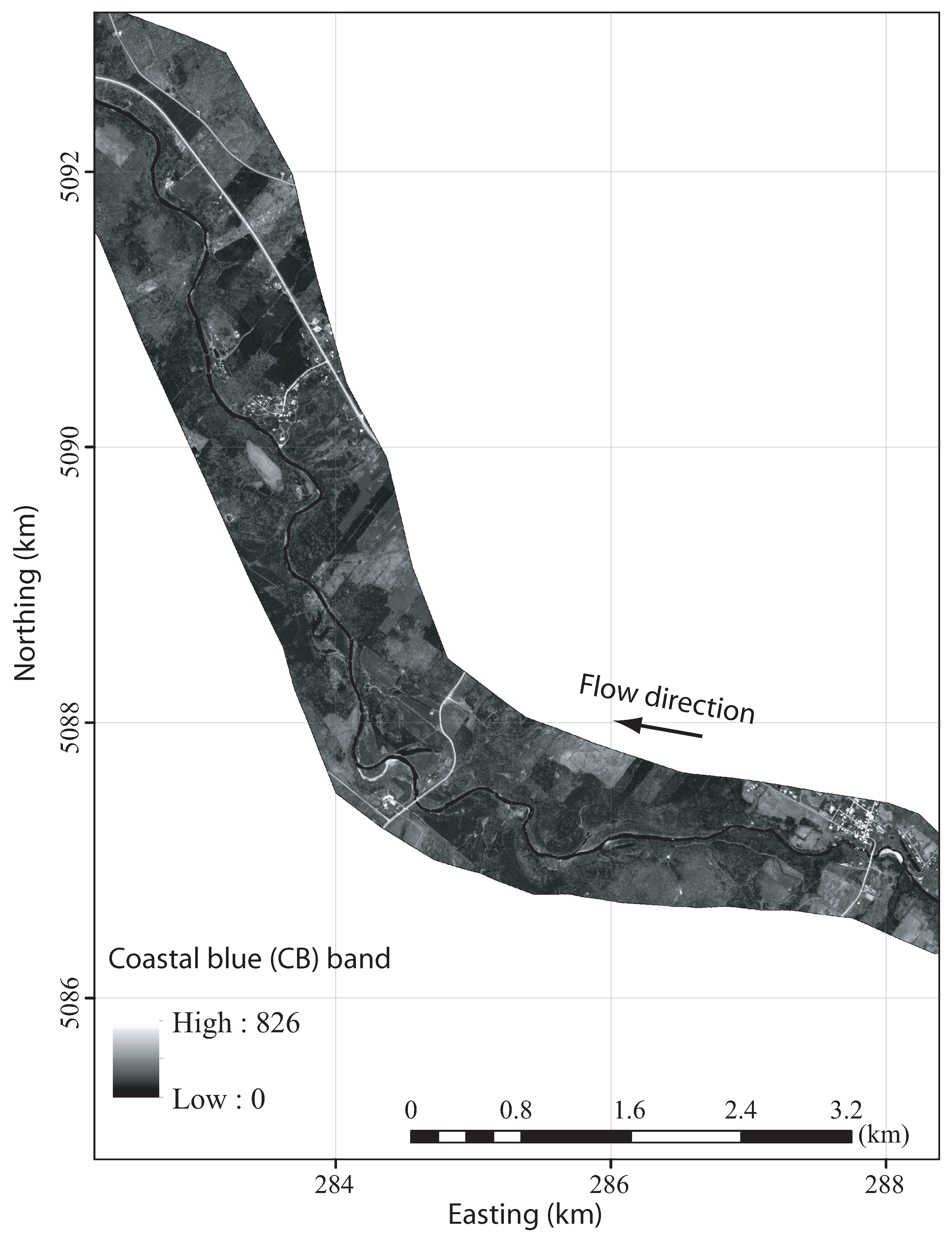
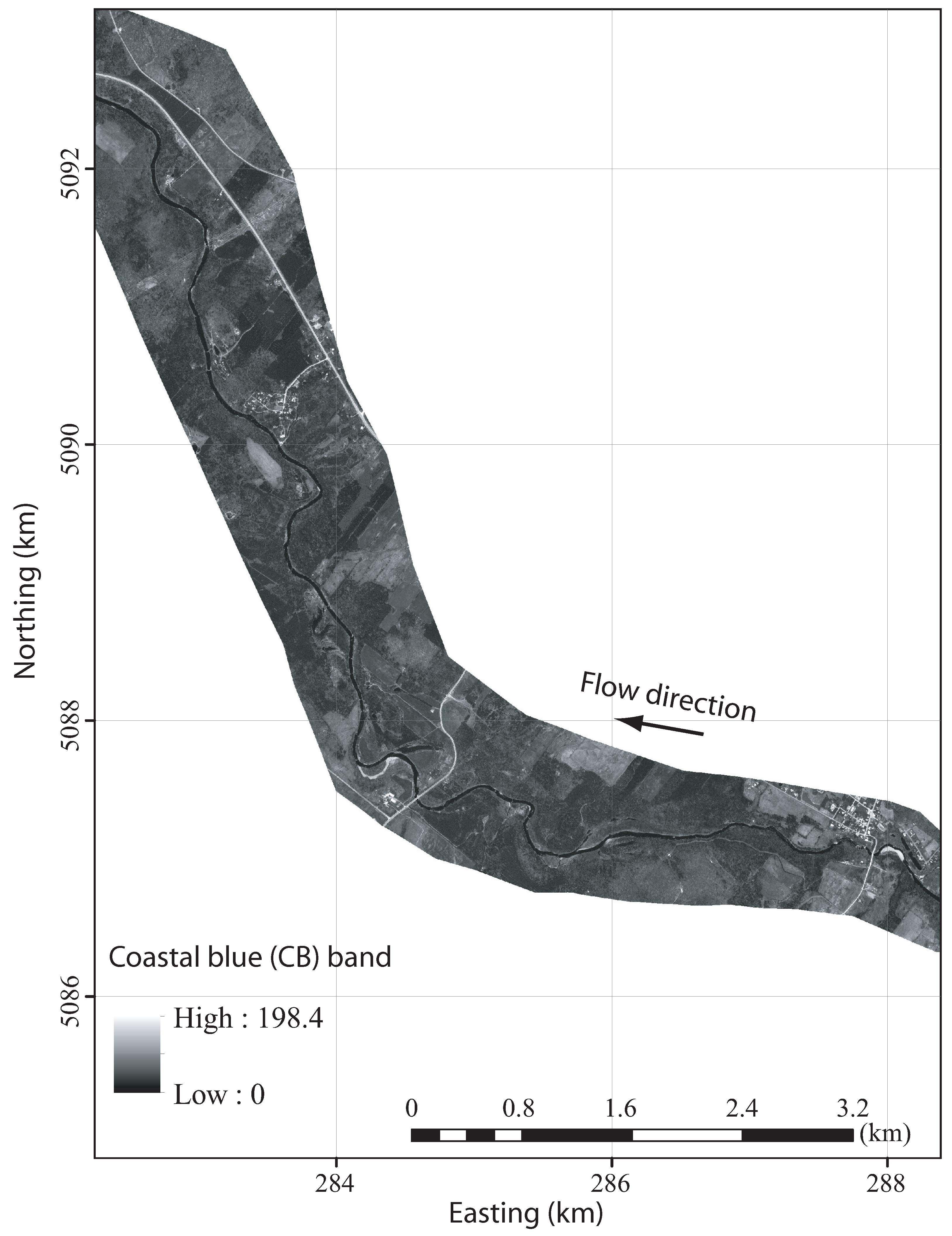
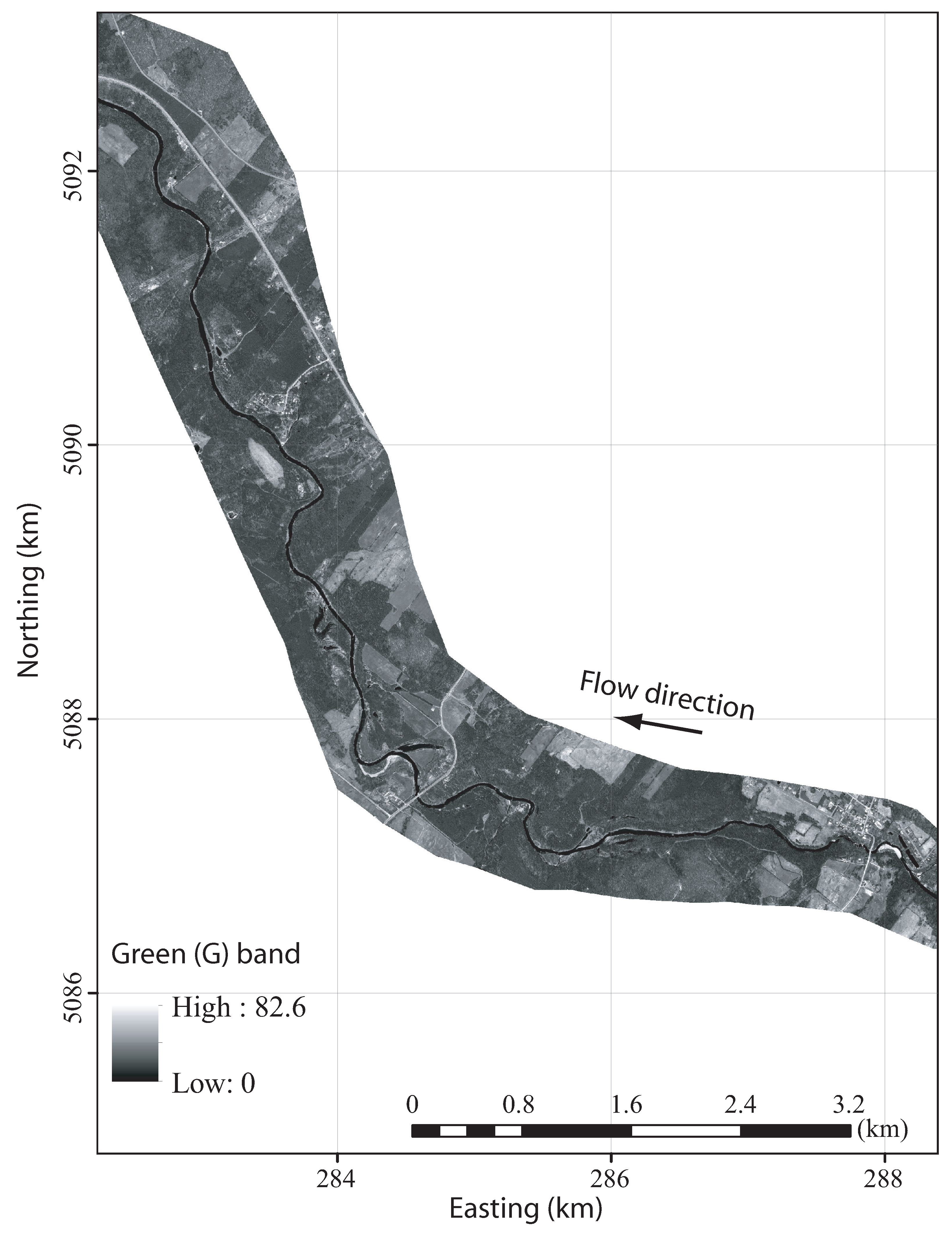
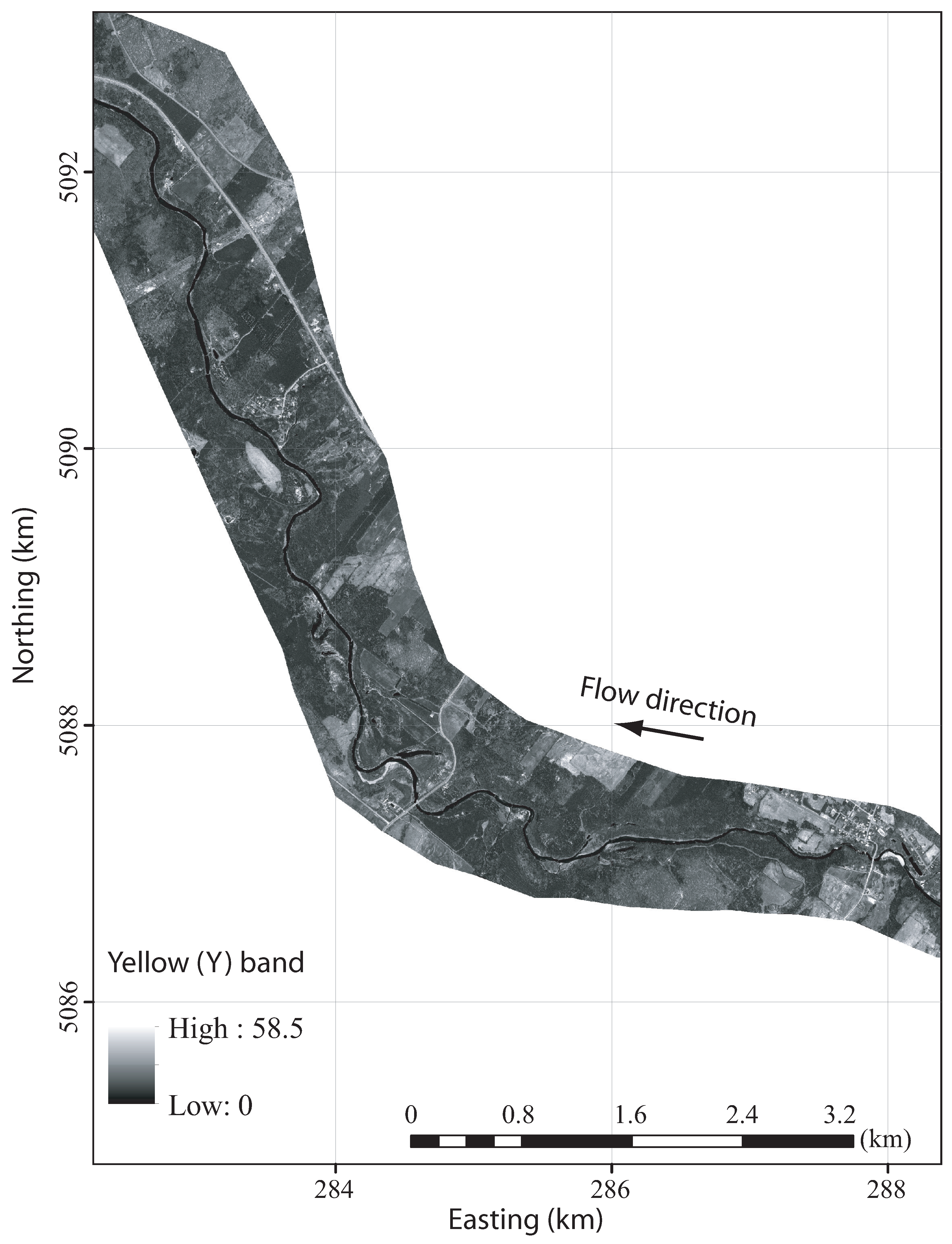
3.1. Digital Number and TOA Reflectance
3.2. Effective Attenuation Coefficient
3.3. Flow Depth
4. Discussion
5. Conclusions
Author Contributions
Funding
Institutional Review Board Statement
Informed Consent Statement
Data Availability Statement
Conflicts of Interest
Abbreviations
| B | Blue |
| CB | Coastal blue |
| CGVD28 | Canadian Geodetic Vertical Datum of 1928 |
| DEM | Digital elevation model |
| LiDAR | Light detection and ranging |
| NI1 | Near infrared 1 |
| NI2 | Near infrared 2 |
| NASA | National Aeronautics and Space Administration of the United States |
| NDWI | Normalised difference water index |
| G | Green |
| R | Red |
| RE | Red edge |
| TOA | Top of atmosphere |
| USGS | United States Geological Survey |
| WV-3 | World View 3 |
| Y | Yellow |
Appendix A


References
- Bora, K.; Kalita, H.M. Determination of best groyne combination for mitigating bank erosion. J. Hydroinformatics 2019, 21, 875–892. [Google Scholar] [CrossRef]
- Boavida, I.; Santos, J.M.; Cortes, R.V.; Pinheiro, A.N.; Ferreira, M.T. Assessment of instream structures for habitat improvement for two critically endangered fish species. Aquat. Ecol. 2011, 45, 113–124. [Google Scholar] [CrossRef]
- Radspinner, R.R.; Diplas, P.; Lightbody, A.F.; Sotiropoulos, F. River training and ecological enhancement potential using in-stream structures. J. Hydraul. Eng. 2010, 136, 967–980. [Google Scholar] [CrossRef]
- Carré, D.M.; Biron, P.M.; Gaskin, S.J. Flow dynamics and bedload sediment transport around paired deflectors for fish habitat enhancement: A field study in the Nicolet River. Can. J. Civ. Eng. 2007, 34, 761–769. [Google Scholar] [CrossRef]
- Shields, F.D., Jr.; Cooper, C.M.; Knight, S.S. Experiment in stream restoration. J. Hydraul. Eng. 1995, 121, 494–502. [Google Scholar] [CrossRef]
- Whiteway, S.L.; Biron, P.M.; Zimmermann, A.; Venter, O.; Grant, J.W.A. Do in-stream restoration structures enhance salmonid abundance? A meta-analysis. Can. J. Fish. Aquat. Sci. 2010, 67, 831–841. [Google Scholar] [CrossRef] [Green Version]
- Gong, Z.; Cui, T.; Pu, R.; Lin, C.; Chen, Y. Dynamic simulation of vegetation abundance in a reservoir riparian zone using a sub-pixel Markov model. Int. J. Appl. Earth Obs. Geoinf. 2015, 35, 175–186. [Google Scholar] [CrossRef]
- Smith, K.E.; Terrano, J.F.; Pitchford, J.L.; Archer, M.J. Coastal wetland shoreline change monitoring: A comparison of shorelines from high-resolution WorldView Satellite imagery, aerial Imagery, and field surveys. Remote Sens. 2021, 13, 3030. [Google Scholar] [CrossRef]
- Panteras, G.; Cervone, G. Enhancing the temporal resolution of satellite-based flood extent generation using crowdsourced data for disaster monitoring. Int. J. Remote Sens. 2018, 39, 1459–1474. [Google Scholar] [CrossRef]
- Fan, C. Spectral analysis of water reflectance for hyperspectral remote sensing of water quality in estuarine water. J. Geosci. Environ. Prot. 2014, 2, 19. [Google Scholar]
- Xiong, Y.; Ran, Y.; Zhao, S.; Zhao, H.; Tian, Q. Remotely assessing and monitoring coastal and inland water quality in China: Progress, challenges and outlook. Crit. Rev. Environ. Sci. Technol. 2020, 50, 1266–1302. [Google Scholar] [CrossRef]
- Yang, X.; Sokoletsky, L.; Wei, X.; Shen, F. Suspended sediment concentration mapping based on the MODIS satellite imagery in the East China inland, estuarine, and coastal waters. Chin. J. Oceanol. Limnol. 2017, 35, 39–60. [Google Scholar] [CrossRef]
- Yuzugullu, O.; Aksoy, A. Generation of the bathymetry of a eutrophic shallow lake using WorldView-2 imagery. J. Hydroinformatics 2014, 16, 50–59. [Google Scholar] [CrossRef]
- García de Jalón, D.; Gortazar, J. Evaluation of instream habitat enhancement options using fish habitat simulations: Case-studies in the river Pas (Spain). Aquat. Ecol. 2007, 41, 461–474. [Google Scholar] [CrossRef]
- Lee, J.H.; Kil, J.T.; Jeong, S. Evaluation of physical fish habitat quality enhancement designs in urban streams using a 2D hydrodynamic model. Ecol. Eng. 2010, 36, 1251–1259. [Google Scholar] [CrossRef]
- Vehanen, T.; Huusko, A.; Yrjänä, T.; Lahti, M.; Mäki-Petäys, A. Habitat preference by grayling (Thymallus thymallus) in an artificially modified, hydropeaking riverbed: A contribution to understand the effectiveness of habitat enhancement measures. J. Appl. Ichthyol. 2003, 19, 15–20. [Google Scholar] [CrossRef]
- Legleiter, C.J.; Roberts, D.A.; Lawrence, R.L. Spectrally based remote sensing of river bathymetry. Earth Surf. Process. Landforms 2009, 34, 1039–1059. [Google Scholar] [CrossRef]
- Niroumand-Jadidi, M.; Bovolo, F.; Bruzzone, L. SMART-SDB: Sample-specific multiple band ratio technique for satellite-derived bathymetry. Remote Sens. Environ. 2020, 251, 112091. [Google Scholar] [CrossRef]
- Legleiter, C.J.; Overstreet, B.T. Mapping gravel bed river bathymetry from space. J. Geophys. Res. Earth Surf. 2012, 117, F04024. [Google Scholar] [CrossRef]
- Harada, S.; Li, S.S. Combining remote sensing with physical flow laws to estimate river channel geometry. River Res. Appl. 2018, 34, 697–708. [Google Scholar] [CrossRef]
- Hugue, F.; Lapointe, M.; Eaton, B.C.; Lepoutre, A. Satellite-based remote sensing of running water habitats at large riverscape scales: Tools to analyze habitat heterogeneity for river ecosystem management. Geomorphology 2016, 253, 353–369. [Google Scholar] [CrossRef]
- Niroumand-Jadidi, M.; Vitti, A. Optimal band ratio analysis of WorldView-3 imagery for bathymetry of shallow rivers (case study: Sarca River, Italy). In Proceedings of the XXIII ISPRS Congress, Prague, Czech Republic, 12–19 July 2016; pp. 361–365. [Google Scholar]
- Parente, C.; Pepe, M. Bathymetry from WorldView-3 satellite data using radiometric band ratio. Acta Polytech. 2018, 58, 109–117. [Google Scholar] [CrossRef] [Green Version]
- Bierwirth, P.N.; Lee, T.J.; Burne, R.V. Shallow sea-floor reflectance and water depth derived by unmixing multispectral imagery. Photogramm. Eng. Remote Sens. 1993, 59, 6185017. [Google Scholar]
- Collin, A.; Etienne, S.; Feunteun, E. VHR coastal bathymetry using WorldView-3: Colour versus learner. Remote Sens. Lett. 2017, 8, 1072–1081. [Google Scholar] [CrossRef]
- Stumpf, R.P.; Holderied, K.; Sinclair, M. Determination of water depth with high-resolution satellite imagery over variable bottom types. Limnol. Oceanogr. 2003, 48, 547–556. [Google Scholar] [CrossRef]
- Tripathi, N.K.; Rao, A.M. Bathymetric mapping in Kakinada Bay, India, using IRS-1D LISS-III data. Int. J. Remote Sens. 2002, 23, 1013–1025. [Google Scholar] [CrossRef]
- Carré, D.M. Flow Dynamics and Bedload Sediment Transport around Paired Deflectors for Fish Habitat Enhancement. Ph.D. Thesis, McGill University, Montreal, QC, Canada, 2011. [Google Scholar]
- Whiteway, S.L. Assessing the Effectiveness of Instream Structures for Restoring Salmonid Streams. Master’s Thesis, Concordia University, Montreal, QC, Canada, 2009. [Google Scholar]
- Biron, P.M.; Chone, G.; Buffin-Belanger, T.; Demers, S.; Olsen, T. Improvement of streams hydro-geomorphological assessment using LiDAR DEMs. Earth Surf. Process. Landforms 2013, 38, 1808–1821. [Google Scholar] [CrossRef]
- Ng, K.P.T. Two-dimensional Hydraulic-habitat Modeling of a Rehabilitated River. Master’s Thesis, McGill University, Montreal, QC, Canada, 2005. [Google Scholar]
- Janzen, D.T.; Fredeen, A.L.; Wheate, R.D. Radiometric correction techniques and accuracy assessment for Landsat TM data in remote forested regions. Can. J. Remote Sens. 2006, 32, 330–340. [Google Scholar] [CrossRef]
- Kuester, M. Radiometric Use of WorldView-3 Imagery; Technical Note; DigitalGlobe: Longmont, CO, USA, 2016. [Google Scholar]
- McFeeters, S.K. The use of the normalized difference water index (NDWI) in the delineation of open water features. Int. J. Remote Sens. 1996, 17, 1425–1432. [Google Scholar] [CrossRef]
- Lee, Z.P.; Du, K.P.; Arnone, R. A model for the diffuse attenuation coefficient of downwelling irradiance. J. Geophys. Res. Ocean. 2005, 110, C02016. [Google Scholar] [CrossRef]
- Lee, Z.; Carder, K.L.; Arnone, R.A. Deriving inherent optical properties from water color: A multiband quasi-analytical algorithm for optically deep waters. Appl. Opt. 2002, 41, 5755–5772. [Google Scholar] [CrossRef] [PubMed]
- Chen, J.F.; Zagzebski, J.A.; Madsen, E.L. Tests of backscatter coefficient measurement using broadband pulses. IEEE Trans. Ultrason. Ferroelectr. Freq. Control 1993, 40, 603–607. [Google Scholar] [CrossRef] [PubMed]
- Morel, A. Optical properties of pure water and pure sea water. In Proceedings of the Symposium on Optical Aspects of Oceanography, Copenhagen, Denmark, 19–23 June 1972. [Google Scholar]
- Buiteveld, H.; Hakvoort, J.H.M.; Donze, M. Optical properties of pure water. In Proceedings of the Ocean Optics XII, Bergen, Norway, 22 October 1994; Volume 2258, pp. 174–183. [Google Scholar]
- Baban, S.M. The evaluation of different algorithms for bathymetric charting of lakes using Landsat imagery. Int. J. Remote Sens. 1993, 14, 2263–2273. [Google Scholar] [CrossRef]
- Updike, T.; Comp, C. Radiometric Use of WorldView-2 Imagery; Technical Note; DigitalGlobe: Longmont, CO, USA, 2010; pp. 1–17. [Google Scholar]
- Jawak, S.D.; Luis, A.J. Spectral information analysis for the semiautomatic derivation of shallow lake bathymetry using high-resolution multispectral imagery: A case study of Antarctic coastal oasis. Aquat. Procedia 2015, 4, 1331–1338. [Google Scholar] [CrossRef]


| Band | λ | Δλ | λo | E | g | o | c |
|---|---|---|---|---|---|---|---|
| nm | μm | nm | W/(m2μm) | W/(m2μm) | W/(m2sr-Count) | ||
| CB | 400–450 | 0.0405 | 427.4 | 1743.8 | 0.2909 | −7.070 | 0.0139747 |
| B | 450–510 | 0.054 | 481.9 | 1971.5 | 0.3052 | −4.253 | 0.0177236 |
| G | 510–580 | 0.0618 | 555 | 1856.3 | 0.1955 | −2.633 | 0.0131636 |
| Y | 585–625 | 0.0381 | 604.3 | 1749.4 | 0.1679 | −2.074 | 0.0067200 |
| R | 630–690 | 0.0585 | 660.1 | 1555.1 | 0.1695 | −1.807 | 0.0102036 |
| RE | 705–745 | 0.0387 | 1344.0 | 0.1560 | −2.633 | 0.0060632 | |
| NI1 | 770–895 | 0.1004 | 1072.0 | 0.1159 | −3.406 | 0.0117091 | |
| NI2 | 860–1040 | 0.0899 | 863.3 | 0.1193 | −2.258 | 0.0103495 |
| Case | a | b | ||
|---|---|---|---|---|
| (m) | (m) | (m) | (%) | |
| Base case | 0.0677 | 8.0533 | 25.3232 | 0% |
| Case 1 | 0.0684 | 8.0533 | 25.3853 | 0.25% |
| Case 2 | 0.0711 | 8.0533 | 25.6296 | 1.21% |
| Case 3 | 0.0677 | 8.1353 | 25.5756 | 1.00% |
| Case 4 | 0.0677 | 8.4575 | 26.5855 | 4.98% |
Publisher’s Note: MDPI stays neutral with regard to jurisdictional claims in published maps and institutional affiliations. |
© 2022 by the authors. Licensee MDPI, Basel, Switzerland. This article is an open access article distributed under the terms and conditions of the Creative Commons Attribution (CC BY) license (https://creativecommons.org/licenses/by/4.0/).
Share and Cite
Salavitabar, S.; Li, S.S.; Lak, B. Mapping Underwater Bathymetry of a Shallow River from Satellite Multispectral Imagery. Geosciences 2022, 12, 142. https://doi.org/10.3390/geosciences12040142
Salavitabar S, Li SS, Lak B. Mapping Underwater Bathymetry of a Shallow River from Satellite Multispectral Imagery. Geosciences. 2022; 12(4):142. https://doi.org/10.3390/geosciences12040142
Chicago/Turabian StyleSalavitabar, Shayan, S. Samuel Li, and Behzad Lak. 2022. "Mapping Underwater Bathymetry of a Shallow River from Satellite Multispectral Imagery" Geosciences 12, no. 4: 142. https://doi.org/10.3390/geosciences12040142