Atmospheric pCO₂ Reconstruction of Early Cretaceous Terrestrial Deposits in Texas and Oklahoma Using Pedogenic Carbonate and Occluded Organic Matter

Abstract

Pedogenic carbonate samples collected from three Lower Cretaceous (Aptian–Albian) fossil localities in Texas and Oklahoma were analyzed to develop paleoatmospheric pCO₂ estimates by measuring the stable carbon isotopes of pedogenic calcite and their co-existing occluded organic matter. Calcite δ¹³C values ranged from −10.9‰ to −4.4‰ while occluded organic matter δ¹³C values ranged from −27.3‰ to −21.1‰. These stable carbon isotope measurements combined with temperature (30 °C) and soil-respired CO₂ concentration (839–6047 ppmV) values provided atmospheric pCO₂ estimates ranging from 67 ppmV to over 1100 ppmV. These estimates show a significant increase in atmospheric pCO₂ during the late Aptian followed by a decrease in atmospheric pCO₂ during the late Aptian to early Albian transition period, roughly correlating with the OEA1b event. Given the lack of chronostratigraphic constraints of the Lower Cretaceous geologic units in the study area, these data provide further evidence for the approximate age of the units as well as pertinent paleoclimate insights into greenhouse climate conditions.

1. Introduction

The Cretaceous climate has long been an area of keen interest as computer-based models and proxy-based paleoclimatic studies aim to understand this “greenhouse” period. Recently, the terrestrial carbon isotope record has become a major contributing factor in discovering the correlation between shifts in Earth’s near-surface global carbon δ¹³C compositions, including oceanic anoxic events (OAEs), and its relationship to changes in climate during the Early Cretaceous [1,2,3,4,5]. Here, we present data from paleosol calcite from the Aptian–Albian terrestrial units of Texas and Oklahoma in an effort to understand changes in atmospheric pCO₂ and its correlation(s) with regional and potentially global climatic changes, as deduced from independent geochemical proxies within these paleosols, including paleoprecipitation and paleotemperature, as well as other paleoenvironmental and paleoclimatic information offered by previously published work on Lower Cretaceous deposits. Furthermore, we aim to understand the correlation between changes in estimated atmospheric pCO₂ levels and global ocean–atmospheric events identified during the Aptian–Albian period.

2. Materials and Methods

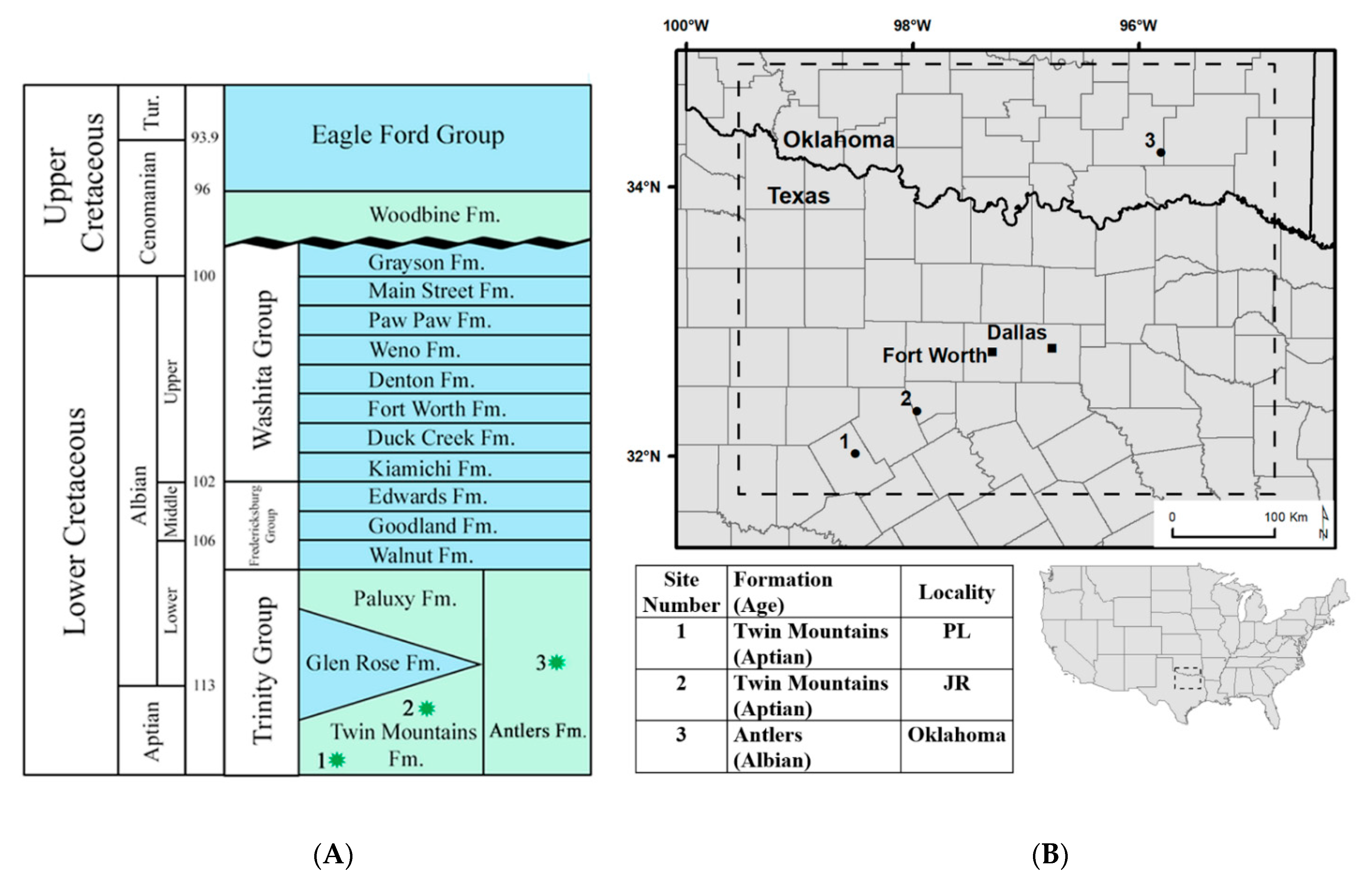
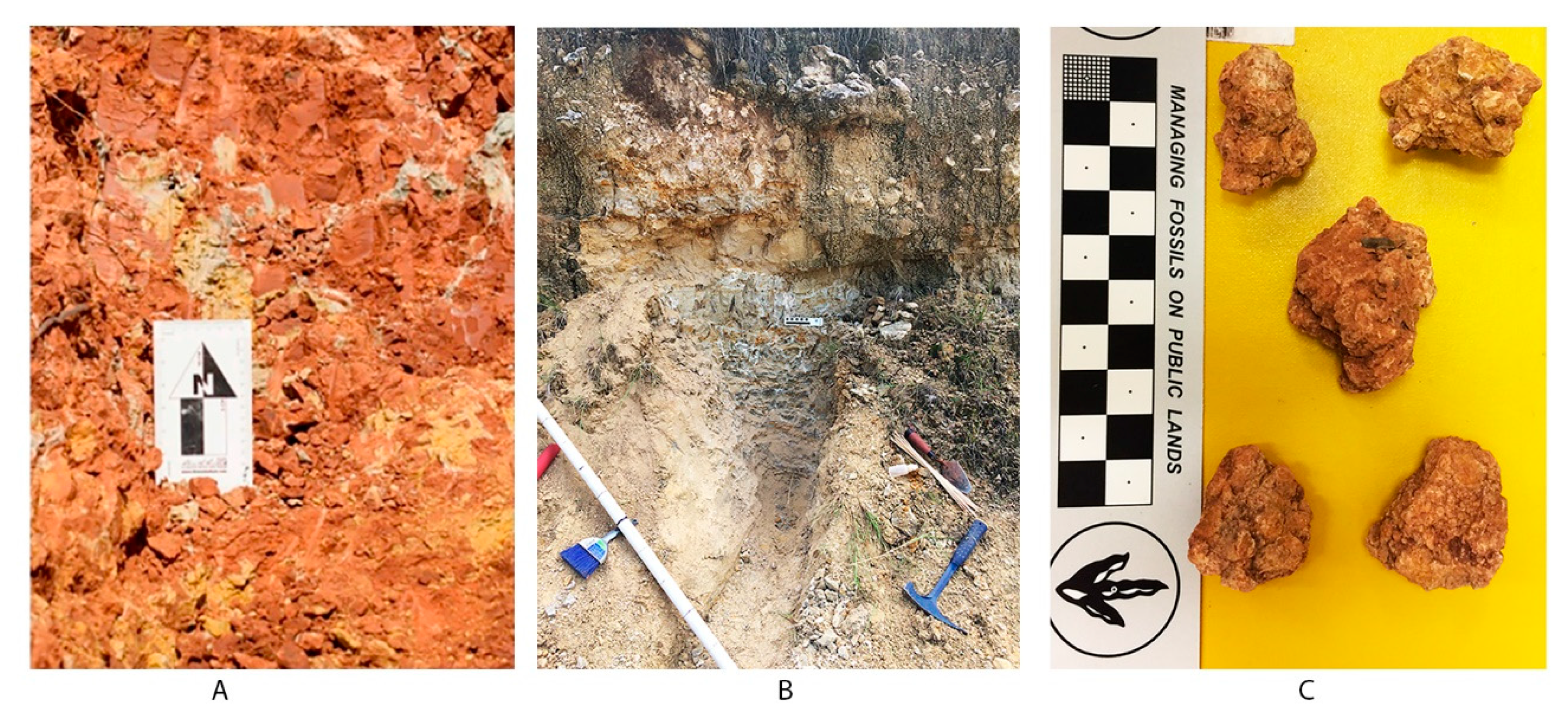
2.1. Geologic Setting

Three localities were sampled for this study, spanning the Lower Cretaceous (Aptian–Albian) stratigraphy of North Central Texas and southern Oklahoma. The precise correlation of these localities is difficult as the succession includes the time-transgressive progradational and retrogradational sequences of the Western Interior Seaway, which have produced a complicated succession of interfingering carbonates, mudstones, sandstones, and rare coals that are reflective of both continental and marine facies. Nevertheless, the stratigraphic analysis by Jacobs and Winkler [6] (Figure 1) provided sufficient constraints to place these localities within a framework that ensures chronological order and biostratigraphic separation at the geological stage scale, albeit without chronometric dates.

The Twin Mountains Formation lies unconformably upon Pennsylvanian and Permian strata and represents the lowest Cretaceous deposits in North Central Texas [7]. Ammonite faunas are used to define the Aptian–Albian boundary in the overlying Glen Rose Formation [7,8,9,10]. Paleomagnetic studies of the Twin Mountains Formation have indicated normal polarity, which correlates to a long normal quiet zone during the Aptian and Albian stages [11,12]. The combination of the overlying biostratigraphic marker in the marine-dominated Glen Rose Formation and the paleomagnetic data collected from the Twin Mountains Formation indicates that the Twin Mountains Formation is Aptian in age. The exposures of the formation have been interpreted as sedimentary deposits of meander belt fluvial systems that transition stratigraphically upward to marginal marine deposits [13].

Paleosols from the Twin Mountains Formation were sampled at two fossil localities: Proctor Lake and Jones Ranch (Figure 1, sites 1 and 2). Paleosols at the Proctor Lake locality were first discovered during the excavation of fossil material from Convolosaurus marri, a basal ornithopod dinosaur [14]. The locality lies in the lower Twin Mountains Formation, approximately 17 m above the Pennsylvanian contact and 35 m below the Glen Rose Formation contact [15]. Pedogenic carbonate nodules measuring 3–5cm in diameter were recovered from a single Bk horizon in the lower section of the 3.2 m paleosol profile. These samples were labeled PL-3, PL-6, and PL-8. The observed paleosols consisted of a series of stacked B horizons and were previously classified as vertic Calcisols that contain prismatic peds, highly reactive carbonate matrix, infill dikes, and vermicular mottles [16] (Figure 2).

The Jones Ranch fossil locality occurs stratigraphically higher in the Twin Mountains Formation than the Proctor Lake locality, correlating with localities that are latest Aptian–early Albian in age (~113 Ma) [6,15,17,18]. A previous sedimentological study of the strata associated with the Jones Ranch fossil quarry interpreted the dinosaur-bearing strata as having been a broad and shallow ephemeral fluvial channel that occurred ~9.7 m below the Twin Mountains Formation’s upper contact with the Glen Rose Formation [18]. The dinosaur-bearing strata at the quarry consist of a lower, 40-cm thick bed that scours the underlying unfossiliferous stratum and fines upward from a basal concretionary sandstone with clay rip-up clasts to trough cross-bedded sandstone and an upper, 30-cm thick bed of cross-bedded sandstone with lenticular mud drapes and abundant fossil charcoal, wood, tree trunks up to 6 m in length, and plant debris. The 80-cm thick unit of fine-grained sandstones overlying the bone-bearing strata has a massive to single-grain soil texture and preserves the calcareous nodules and tubules that are interpreted to be the products of pedogenesis in a semi-arid climate (i.e., a paleosol, [18], Figure 2). These calcareous tubules from the paleosol profile were collected for geochemical study. The tubules are concentrated in 50 cm of outcrop and occur as irregular but continuous cylinders of micritic calcite with a uniform diameter of ~5–8 mm and common, small (1–2 mm diameter) channels of carbonate that extend outward along the length of and perpendicular to the main cylinder. The 13 calcareous tubules, labeled CR1–CR13, that were collected from the outcrop all had similar diameters (~5–8 mm) but ranged in length from ~20 mm to 75 mm. These tubules were interpreted as being root petrifactions (i.e., rhizoliths, [19]) that formed around and replaced root systems in the soil during Early Cretaceous pedogenesis.

The Twin Mountains and Paluxy Formations, both of which are interpreted as representing littoral to continental sedimentary deposits, are separated by the marine-dominated sedimentary rocks of the Glen Rose Formation in the southern part of the study area (Figure 1). To the north, the marine-dominated Glen Rose Formation pinches out and the continental-dominated Twin Mountains and Paluxy Formations combine to form the Antlers Formation (Figure 1), which contains claystone layers with unconsolidated sandstone lenses and carbonate concretions that have been interpreted as representing fluvial, deltaic, and strandplain settings [17,20]. The vertebrate fauna of the Antlers Formation is similar to that of the Twin Mountains and Paluxy Formations [21].

The precise stratigraphic positions of localities within the Antlers Formation are difficult to determine because of the absence of the Glen Rose Formation as a marker. The locality sampled in Oklahoma is stratigraphically equivalent with sections measured at fossil locality OMNH V706, which is considered to be in the middle Antlers Formation, occurring ~87 m above the base [22] (Figure 1, site 3). The stable carbon isotope ratios from fossil wood at this site are consistent with those from the middle of the Glen Rose Formation, which is considered to be Early Albian in age, based upon a stable carbon isotope chemostratigraphic correlation between Cretaceous vascular plant organic matter and shallow marine calcite [23]. The paleosol profile, identified as a calcic Vertisol, measures 2.36 m in thickness with fine to medium wedge-shaped peds that collectively define large arcuate slickenplanes at depth within the profile [16]. Pedogenic carbonate nodules up to 5 cm in diameter were collected from a single Bk horizon and were labeled as Cross-C1, Cross-C9, and Cross-C10 (Figure 2). All discrete pedogenic nodules and calcareous rhizoliths were collected from depths greater than 50cm below the ancient soil surface, ensuring consistency in the isotopic composition and the pressure of soil CO₂ [24,25].

2.2. Laboratory Methods

Aliquots of each sample were ground separately with a corundum mortar and pestle to pass through a <62 µm sieve. To verify that the carbonate samples contained only low-Mg calcite, the samples were analyzed by powder X-ray diffraction using a Rigaku Ultima III X-ray diffractometer equipped with a Cu–Ka radiation X-ray source at Southern Methodist University (SMU). X-ray scans ranged from 2–70° 2θ with step lengths of 0.04° 2θ and at a rate of 1° 2θ/min. Another aliquot of each section was prepared as petrographic thin sections (~100 μm thick) and stained using alizarin red-S in order to confirm the presence of calcite. Each thin section was inspected with its matching billet under a reflected light microscope in order to verify that micrite (~<20 µm carbonate crystal size) was the only cement texture present and that later diagenetic textures, such as sparry calcite or dolomite cements, were absent. The samples selected for further analyses contained only micritic low-Mg calcite. The powders that were used for the X-ray diffraction analyses were then used as materials for the determination of pedogenic carbonate and co-existing occluded organic matter δ¹³C values, as described below.

Paleosol carbonate powders from each sample were split into two fractions: one fraction that underwent no further chemical pretreatments, which was analyzed for calcite δ¹³C and δ ¹⁸O values (see below), and a second fraction that was acidified in concentrated (~12 N) HCl solution. Each acid-treated fraction (

Table 1. The paleosol carbonate stable isotopic values of the measured δ¹³C of calcite (δ¹³C_carb‰ VPDB), the measured δ¹³C of acid-treated residues containing occluded organic matter (δ¹³C_oom‰ VPDB), the differences between paired calcite and co-existing occluded organic matter (Δ¹³C_cc-om), and the estimated δ¹³C of soil-respired CO₂ at the time of calcite crystallization (δ¹³C_S) based on the measured values of the occluded organic matter corrected for diffusion enrichment assuming a soil temperature of 30 °C (δ¹³C_S‰ VPDB, 30 °C). Replicate analyses are marked with “R”.

Location	Sample	Formation (Age)	δ13Ccarb (‰ VPDB)	δ13Coom (‰ VPDB)	Δ13Ccc-om (‰)	δ13CS (‰ VPDB, 30 °C)
Oklahoma	Cross-C-10	Antlers	−10.84	−25.22	14.38	−12.55
	Cross C-9	(Albian)	−10.93	−25.87	14.94	−13.20
	Cross C-1		−10.92	−25.00	14.08	−12.33
Jones Ranch, TX
	CR13A	Twin Mountains	−4.72	−24.70	19.98	−12.03
	CR13B	(Aptian)	−4.39	−24.70	20.31	−12.03
	CR12A		−5.12	−23.75	18.63	−11.07
	CR12B		−4.99	−23.75	18.76	−11.07
	CR11A		−5.18	−26.05	20.87	−13.38
	CR11B		−5.19	−26.05	20.86	−13.38
	CR10A		−4.92	−23.85	18.93	−11.17
	CR10B		−5.13	−23.85	18.72	−11.17
	CR9A		−5.96	−24.87	18.91	−12.20
	CR9B		−6.01	−24.87	18.86	−12.20
	CR8A		−5.56	−24.59	19.03	−11.92
	CR8B		−5.32	−24.59	19.27	−11.92
	CR7A		−5.12	−23.77	18.65	−11.09
	CR7B		−5.42	−23.77	18.35	−11.09
	CR6B		−5.91	−26.02	20.11	−13.35
	CR5A		−5.61	−24.16	18.55	−11.49
	CR5B		−5.59	−24.16	18.57	−11.49
	CR4A		−5.49	−27.30	21.81	−14.64
	CR4B		−5.64	−27.30	21.66	−14.64
	CR3A		−5.54	−23.53	17.99	−10.85
	CR3B		−5.70	−23.53	17.83	−10.85
	CR2A		−5.71	−27.03	21.32	−14.37
	CR2A-R		−5.56	−27.03	21.47	−14.37
	CR2B		−5.67	−27.03	21.36	−14.37
	CR1A		−5.89	−23.20	17.31	−10.52
	CR1A-R		−5.89	−23.20	17.31	−10.52
	CR1B		−5.67	−23.20	17.53	−10.52
Proctor Lake, TX
	PL-8	Twin Mountains	−7.84	−21.08	13.24	−8.39
	PL-6	(Aptian)	−7.77	−21.43	13.66	−8.74
	PL-3		−8.00	−21.39	13.39	−8.70

) was kept in contact with ~12 N HCl solution for at least 24 h and fresh aliquots of ~12 N HCl solution were introduced to these fractions every 12 h until no effervescence could be detected. These acid-treated fractions were then rinsed with de-ionized H₂O until the rinse water remained at the original pH of the de-ionized H₂O (~5.6) after at least 10 min of contact with the acid-leached residue. The acid pretreatment of these fractions was designed to remove carbonate minerals from the samples and concentrate any finely disseminated occluded organic matter within the acid-treated residue. The carbon concentration and δ¹³C values of these samples were determined from the CO₂ produced by the closed system combustion of the organic matter, following the methods of Boutton [26]. Gas samples produced by the combustion were cryogenically purified to isolate CO₂ and the CO₂ yields were measured via mercury manometry, with a precision of ± 0.2 µmol, using high-vacuum glass extraction lines at SMU.

For the determination of the calcite δ¹³C and δ¹⁸O values, between 10.0 and 19.2 mg of carbonate-bearing powders were loaded into reaction vessels and their atmospheric gases were evacuated. The samples were then dissolved in 100% H₃PO₄ in vacuo at 25 °C for ~16 h to produce CO₂. The CO₂ samples resulting from the acid dissolution of the calcite were cryogenically purified to isolate CO₂ and the CO₂ yields were measured via mercury manometry, with a precision of ± 0.2 µmol, using high-vacuum glass extraction lines at SMU. The CO₂ resulting from the combustion of acid-treated residue fractions, as well as all of the aliquots of the calcareous tubules, were analyzed for carbon and oxygen stable isotope ratios using a Finnigan MAT 253 isotope ratio mass spectrometer at SMU. The carbon and oxygen isotope values are reported in per mille notation and “std” corresponds to the Vienna Peedee Belemnite (V-PDB) standard [27,28].

2.3. Estimating Atmospheric CO₂

The atmospheric pCO₂ estimates were made using the δ¹³C values measured from the pedogenic calcite and occluded organic matter in combination with a reformulated version of a two-component mixing equation [29]:

$${\mathrm{C}}_{\mathrm{A}}={\mathrm{C}}_{\mathrm{S}}\times \frac{{\mathsf{\delta }}^{13}{\mathrm{C}}_{\mathrm{m}\left(\mathrm{cc}\right)}-{\mathsf{\delta }}^{13}{\mathrm{C}}_{\mathrm{O}\left(\mathrm{cc}\right)}}{{\mathsf{\delta }}^{13}{\mathrm{C}}_{\mathrm{A}\left(\mathrm{cc}\right)}-{\mathsf{\delta }}^{13}{\mathrm{C}}_{\mathrm{O}\left(\mathrm{cc}\right)}}$$

(1)

where C_A is the concentration of atmospheric CO₂ in ppmV, C_S is the concentration of soil CO₂ in ppmV, δ¹³C_O(cc) is the δ¹³C of calcite precipitated in equilibrium with only soil-respired CO₂, δ¹³C_A(cc) is the δ¹³C value of calcite precipitated in equilibrium with only atmospheric CO₂, and δ¹³C_m(cc) is the measured δ¹³C value of pedogenic calcite that precipitated in equilibrium with soil CO₂, which is a mixture of atmospheric and soil-respired CO₂.

To calculate the atmospheric pCO₂ estimates, this equation required assumptions for the soil pCO₂, the δ¹³C of the atmosphere, and the soil temperature at the time(s) of calcite crystallization in the soil. A value of −6.5‰ was chosen for the δ¹³C value of Early Cretaceous paleoatmospheric CO₂ [2,25,30,31,32,33]. A soil temperature of 30 °C was chosen based on paleotemperature estimates derived from the oxygen and hydrogen isotope analyses of pedogenic phyllosilicates from the paleosols associated with each locality considered here [16]. The measured δ¹³C of occluded organic matter was related to the δ¹³C of soil-respired CO₂ [25]; however, the δ ¹³C of the occluded organic matter had to be corrected to account for the upward carbon isotope diffusion of the soil-respired CO₂ through the soil profile, which causes an enrichment in ¹³C of at least 4.4‰ [34]. This was estimated using the following equation [35,36,37,38]:

$${\mathsf{\delta }}^{13}{\mathrm{C}}_{{\mathrm{CO}}_2}={1.0044\mathsf{\delta }}^{13}{\mathrm{C}}_{\mathrm{OM}}+4.4$$

(2)

where δ¹³C_CO2 is the diffusion-corrected δ¹³C value of soil-respired CO₂ and ¹³C_OM is the measured δ¹³C value of organic matter for the acid-treated residues (i.e., uncorrected soil-respired CO₂). The temperature-dependent, stable carbon isotope, calcite–CO₂ enrichment factor was then applied to the diffusion corrected δ¹³C_CO2 to calculate δ¹³C_O(cc) using the following equation [39]:

$${\mathsf{\epsilon }}_{\mathrm{cc}}{-\mathrm{CO}}_2=11.98-0.12\times \mathrm{T}(°\mathrm{C})$$

This same enrichment factor was also applied to calculate the δ¹³C_A(cc) value used in the two-component mixing equation described above.

The contribution of soil-respired CO₂ (Cs) was a significant source of uncertainty when estimating atmospheric pCO₂. Various levels of soil pCO₂, ranging from 1000 ppmV to 6000 ppmV, have been used throughout the literature to estimate atmospheric pCO₂ levels in the Early Cretaceous [2,4,25,32]. We present two models that used the following soil pCO₂ values: 1250 ppmV and 2000 ppmV. This range was supported by applying methods outlined by Cotton and Sheldon [40], who estimated Cs using mean annual precipitation in modern soils with the following equation:

$$\mathrm{Cs}=5.67\times \mathrm{MAP}-269.9$$

(3)

where soil-respired CO₂ (Cs) is in ppm and mean annual precipitation (MAP) is in mm/yr. Using CALMAG data [41] as proxy estimates for MAP, which were initially reported in Andrzejewski and Tabor [16] for the same localities that were sampled for this study, we estimated the minimum and maximum levels of soil-respired CO₂ using the MAP relationship reported by Cotton and Sheldon [40]. However, it was noted that the modern soil dataset used by Cotton and Sheldon [40] did not include humid climate soils, such as Vertisols, which are present in our dataset. Although changes in the soil pCO₂ affected the estimated numeric value of atmospheric pCO₂, the trends and relative difference between the locality estimates remained the same.

Additionally, the mean annual precipitation was estimated using the negative correlation between the Δ¹³C of paired calcite–occluded organic matter samples described in Tabor et al. [42] using the following equation:

$${\Delta }^{13}{\mathrm{C}}_{\mathrm{cc}-\mathrm{om}}=-0.31\times \mathrm{MAP}\left(\mathrm{cm}\right)+25.43$$

(4)

where Δ¹³C_cc-om is the measured difference between the δ¹³C of measured pedogenic calcite and the corresponding occluded organic matter of the analyzed samples. MAP is the mean annual precipitation estimated in cm/yr. It was noted that this correlation was only documented in soils where MAP was < 500 mm/yr [42].

3. Results

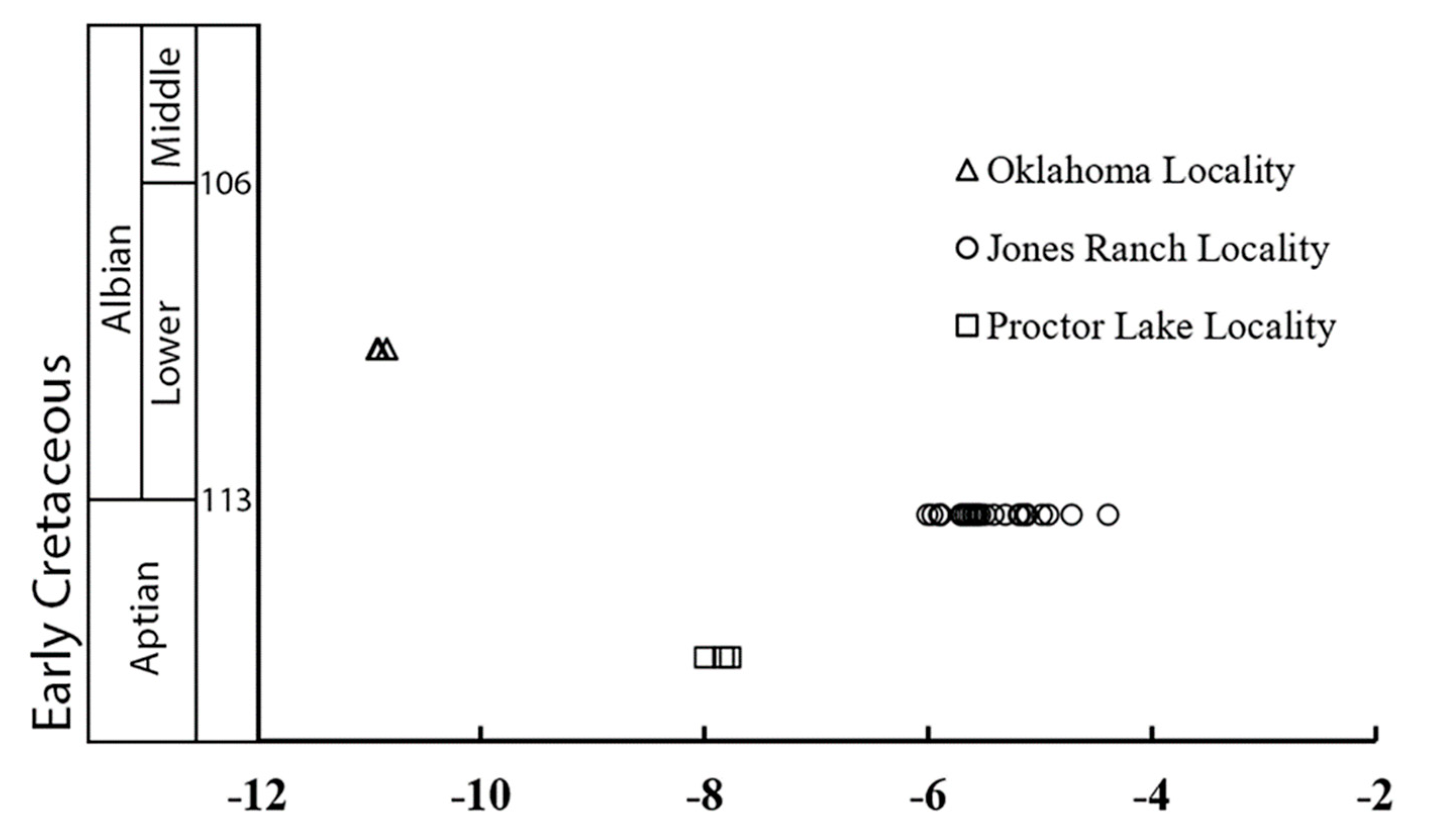
3.1. Pedogenic Carbonate

The results of the 33 analyses of CO₂ derived from the phosphoric acid dissolution of calcite powders among the 19 different calcareous tubules and nodules collected from the Aptian–Albian paleosol profiles are presented in Table 1 and Table S1 and Figure 3. The CO₂ yields from these analyses indicated that the samples ranged from 57 to nearly 100 weight percent calcite, with a mean of 89 ± 11 wt.% (1σ). The calcite δ¹³C values from the Proctor Lake profile ranged from −8.0‰ to −7.8‰ with a mean value of −7.9 ± 0.2 ‰ (1σ), whereas the δ¹⁸O values ranged from −5.8‰ to −4.8‰ with a mean value of −5.1 ± 0.2‰ (1σ). The calcite δ¹³C values from the Jones Ranch profile ranged from −6.0‰ to −4.4‰ with a mean value of −5.4 ± 0.4 ‰ (1σ), whereas the δ¹⁸O values ranged from −4.9‰ to −4.0‰ with a mean value of −4.3 ± 0.2‰ (1σ). The calcite δ¹³C values from the Oklahoma profile ranged from −10.9‰ to −10.8‰ with a mean value of −10.9 ± 0.1 ‰ (1σ), whereas the δ¹⁸O values ranged from −5.8‰ to −5.5‰ with a mean value of −5.6 ± 0.2‰ (1σ). The replicate analyses indicated minimal heterogeneity of the δ¹³C (<0.2‰) and δ¹⁸O (<0.2‰) values in the individual aliquots of calcite powder samples. Similarly, there was minimal heterogeneity of δ¹³C (<0.3‰) and δ¹⁸O (<0.5‰) values between separate aliquots from the same calcareous sample.

3.2. Organic Matter from Acid-Treated Residues

The results of the δ¹³C analysis of organic matter occluded in calcareous tubules and nodules collected from the Aptian–Albian paleosol profiles are presented in Table 1. The CO₂ yields indicated that the acid-treated residues comprised 0.25 to 1.17 weight percent organic carbon (Table S1). The organic residue δ¹³C values ranged from −27.3‰ to −21.1‰ with a mean value of −24.8 ± 1.4‰, which was consistent with the C₃ vegetation that is known to have dominated Early Cretaceous paleolandscapes [43]. The lowest δ¹³C values were from the Proctor Lake locality, averaging −21.3 ± 0.2‰. This was isotopically heavy for C₃ vegetation but fell within the observed range of δ¹³C values for C₃ plants [34]. Modern C₃ plants exhibiting isotopically heavier δ¹³C values are typically water stressed, i.e., there is insufficient soil moisture to support efficient CO₂ uptake through photosynthesis [44]. This observation conformed with previous paleoclimatic studies of the Proctor Lake locality, suggesting it was a semi-arid environment with soil paleotemperatures averaging 30 °C and paleoprecipitation estimates of 330mm/yr [16], which might have induced moisture stress and the relatively heavy organic matter δ¹³C values measured at that locality. In these regards, the δ¹³C values of the occluded organic matter from the Proctor Lake locality are considered reasonable results and are used here to estimate atmospheric pCO₂ levels.

3.3. Mean Annual Precipitation Estimates

The stable carbon isotope differences between the calcite and co-existing occluded organic matter, Δ¹³C_cc-om, ranged from 13.2 to 21.8‰. The resulting Δ¹³C_cc-om values were used as variables in Eqn. 4 in order to yield a corresponding range of MAP estimates from 117 ± 60 mm/yr to 401 ± 30 mm/yr (

Table 2. The mean annual precipitation estimates of Lower Cretaceous localities in Texas and Oklahoma using Δ¹³C_cc-om [42], which are newly presented here, and CALMAG weathering index [41] MAP estimates, as reported in Andrzejewski and Tabor [16]. Soil-respired pCO₂ was then estimated from the mean annual precipitation estimates using the equations derived by Cotton and Sheldon (Equation (3), [40]). C_s¹ calculated soil-respired pCO₂ using MAP derived from Δ¹³C_cc-om. C_s² calculated soil-respired pCO₂ using MAP derived from the CALMAG weathering index.

Locality	Estimate	MAP mm/yr (± 55) Using ΔCcc-om	Cs1 (MAP-Derived)	MAP mm/yr (± 110mm) Using CALMAG	Cs2 (MAP-Derived)
Oklahoma	Min	338	1649	952	5128
	Max	366	1806	1210	6591
	Average	354	1736	1114	6047
Jones Ranch, TX	Min	117	392	288	1363
	Max	262	1215	444	2248
	Average	196	839	365	1800
Proctor Lake, TX	Min	380	1883	268	1250
	Max	401	2004	416	1811
	Average	391	1949	331	1607

, Figure 4). The samples from the Proctor Lake locality averaged 391 ± 30 mm/yr, while samples from the Jones Ranch locality averaged 196 ± 50 mm/yr. The samples collected from the Antlers Formation in Oklahoma averaged 354 ± 40 mm/yr. This suggests that semi-arid climates persisted during the Early Cretaceous in Texas and Oklahoma. The paleoprecipitation estimates reported from these sample localities using CALMAG geochemical weathering indices, which were developed for paleosols, were in close agreement for the Texas localities of Proctor Lake and Jones Ranch; however, the Δ¹³C_cc-om based MAP estimate of ~350 mm/yr contrasted significantly with the CALMAG MAP estimate of ~1100 mm/yr for the Oklahoma locality (Table 2, Figure 4).

There are two possible scenarios that explain the discrepancy between the CALMAG and ∆¹³C_cc-om based MAP estimates of paleoprecipitation from the Oklahoma locality. The first is that the bulk paleosol matrix that was collected and analyzed for the CALMAG analyses contained inherited minerals that were not representative of the original paleosol profile that produced the carbonate nodules. However, work conducted by Andrzejewski and Tabor [16] analyzed the clay mineralogy of the < 0.2 μm fraction of the paleosol matrix, which is thought to represent the authigenic fractions produced in situ, as pedogenic minerals and found substantial amounts of kaolinite in the samples from the Oklahoma locality. This suggests that an interval of increased chemical weathering, which is typically associated with higher rates of meteoric precipitation, supported the higher precipitation estimates produced using the CALMAG weathering index [16]. The second and more plausible scenario is that the paleosol profile recorded two paleoclimate events simultaneously. In this scenario, periods of significant rainfall caused increases in chemical weathering, producing chemically leached minerals, such as kaolinite, which recorded a more humid and high-precipitation paleoclimate, which was detected using the CALMAG weathering index. Additionally, paleosol carbonate precipitates in the soil during a subsequent, younger low-precipitation paleoclimate were detected by the ∆¹³C_cc-om based MAP estimates within the same paleosol profile; this is an example of soil polygenesis and is a common feature in Quaternary-aged modern surfaces [45]. This suggests that the Oklahoma locality might have experienced weather patterns with periods of significant paleoprecipitation that were later followed by much drier periods, during which carbonate precipitated in the paleosol profile. Given that both the CALMAG weathering index and the Δ¹³C_cc-om precipitation proxies provided plausible paleoprecipitation estimates, both were used to estimate soil-respired CO₂ in Table 2. The soil-respired CO₂ estimates were then used to estimate atmospheric pCO₂ in

Table 3. The estimated atmospheric pCO₂ estimates calculated with the C_s values of 1250 and 2000ppmV. The estimated atmospheric pCO₂ values calculated using C_s values based on average mean annual precipitation estimates using the Δ¹³C_cc-om proxy [42] and CALAMG weathering index [41] are shown in the last two columns. The values show the minimum, maximum, and average pCO₂ calculated for each locality.

Locality	Estimate Range	pCO2 (Cs) = 1250	pCO2 (Cs) = 2000	pCO2 (Cs) = Δ13Ccc-om MAP avg.	pCO2 (Cs) = CALMAG MAP avg.
Oklahoma	Min	124	198	172	600
	Max	188	301	261	910
	Average	153	246	213	742
Jones Ranch, TX	Min	467	747	313	671
	Max	692	1108	465	997
	Average	592	947	397	852
Proctor Lake, TX	Min	67	108	105	86
	Max	115	183	179	147
	Average	88	141	138	114

.

3.4. Soil-Respired CO₂ Estimates

Using CALMAG data reported from Andrzejewski and Tabor [16] and MAP estimates made using the Δ¹³C_cc-om precipitation proxy, the minimum and maximum levels of soil-respired CO₂ (Cs) were estimated using the methods outlined by Cotton and Sheldon [40] (Table 2). The lowest reported CALMAG value from the three sampled localities was from the Proctor Lake locality. A measured CALMAG value of 31.0 corresponded to a MAP estimate of 268 mm/yr. By applying the reported relationship between the MAP and soil-respired CO₂, the minimum contribution of soil-respired CO₂ (Cs) was 1250 ppmV. The maximum reported CALMAG values were from the Oklahoma locality, with a CALMAG value of 72.5 producing an MAP estimate of 1210 mm/yr. This MAP estimate produced a maximum contribution of soil-respired CO₂ (Cs) of 6591 ppmV. The lowest MAP estimate produced using the Δ¹³C_cc-om precipitation proxy was 117 mm/yr from the Jones Ranch locality, producing an estimated C_S value of 392 ppmV. The maximum MAP estimate produced using the Δ¹³C_cc-om precipitation proxy was 401 mm/yr from the Proctor Lake locality, producing an estimated C_S value of 2004 ppmV. Given the estimated minimum and maximum values for soil-respired CO₂, we used two different models with Cs values of 1250 and 2000 ppmV to estimate atmospheric pCO₂.

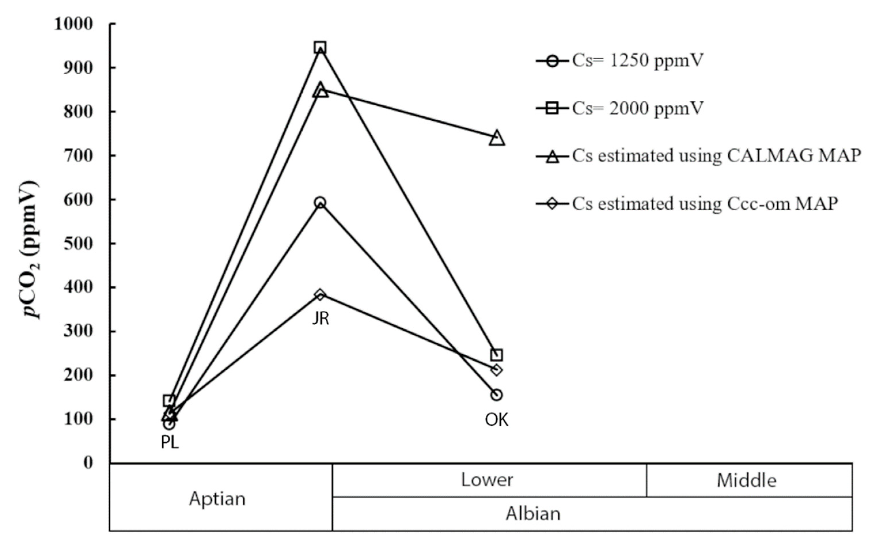
3.5. Atmospheric pCO₂ Estimates

The two models with fixed soil CO₂ values produced estimates of atmospheric pCO₂ ranging from 67 to over 1100 ppmV (Table 3, Figure 5). The largest reported values occurred in samples from the Jones Ranch locality, while lower estimates were produced from the Proctor Lake and Oklahoma localities (Figure 5). Although the absolute value of these estimates significantly changed with the varying estimates of soil-respired pCO₂, the trends were consistent between the two models with differences in atmospheric pCO₂ estimates between the localities remaining proportionally the same. This included an 8-fold increase in atmospheric pCO₂ from the Proctor Lake locality to the Jones Ranch locality, followed by a 4-folddecrease in atmospheric pCO₂ from the Jones Ranch locality to the Oklahoma locality.

The significant increase in atmospheric pCO₂ from the Proctor Lake locality to the Jones Ranch locality was also observed using the locality-specific Cs estimates calculated using the mean annual precipitation estimates. This included the CALMAG index estimates showing an 8-fold increase and the Δ¹³C_cc-om estimates showing a 3-fold increase in atmospheric pCO₂. However, the decrease in atmospheric pCO₂ from the Jones Ranch locality to the Oklahoma locality was far more subtle than the two models with fixed soil CO₂ values, showing an approximately 13% decrease in atmospheric pCO₂ in the CALMAG estimates and a 46% decrease in atmospheric pCO₂ in the Δ¹³C_cc-om estimates. Given the notable difference in soil moisture regimes between the Texas and Oklahoma localities, the Cs values calculated using mean annual precipitation provided a more robust estimate of atmospheric pCO₂ rather than applying the same Cs value to each locality. Although the difference in soil pCO₂ estimates used in these calculations changed the calculated estimates of atmospheric pCO₂ for each locality, the trends produced in all four cases were remarkably similar. This is especially encouraging given that the two proxies used to estimate soil pCO₂ used two different techniques that focused on different aspects of paleosol geochemistry.

4. Discussion

The δ¹³C values of paleosol carbonate reported here are comparable to values recorded in terrestrial carbonates from deposits of a similar age in the Cedar Mountain Formation of Utah [1,4] and Aptian–Albian deposits in China [2,3,5], which have reported δ¹³C values ranging from ~−8.0‰ to −3.0‰. Furthermore, the estimates of atmospheric pCO₂ appear to also agree with Aptian–Albian atmospheric pCO₂ estimates from these regions. More specifically, Ludvigson et al. [4] reported values of 600–1200 ppmV with a soil-respired value (Cs) of 2000 ppmV in the Cedar Mountain Formation in Utah. Li et al. [2] reported atmospheric pCO₂ estimates ranging from 0–5676 ppmV for Cs levels of 2500–5000 ppmV in the Aptian–Albian deposits of southeast China. Moreover, Harper et al. [5] reported atmospheric pCO₂ estimates of 42–1116 ppmV with Cs values ranging from 2427 to 4393 ppmV in the Aptian–Albian deposits of northwest China. Additionally, studies using the stomatal index to estimate atmospheric pCO₂ during the Aptian and Albian periods have reported similar estimates ranging from 450 to 2030 ppmV [46,47,48,49,50]. The significant increase in atmospheric pCO₂ during the late Aptian followed by a decrease in atmospheric pCO₂ across the Aptian–Albian boundary appears to correlate with ocean anoxic event 1b reported during ~113–109 Ma (OAE1b) [51]. While the absence of any true chronostratigraphic constraints in the Texas and Oklahoma stratigraphy prevents us from definitively identifying and assigning a specific isotopic excursion event to this dataset, we recognize that the general pattern of a significant buildup in atmospheric pCO₂ during the late Aptian followed by a decrease in atmospheric pCO₂ during the Aptian–Albian transition and this is strikingly similar to the C10 isotopic excursion identified in the Cedar Mountain Formation [4]. The similarity between these two datasets supports the relative ages assigned to the Texas and Oklahoma localities, as well as the preservation of a global atmospheric change recorded within these sedimentary strata, despite the lack of a true chronostratigraphic framework.

Previous sedimentological and paleoclimatic studies from the Aptian Proctor Lake and Jones Ranch localities have suggested warm, semi-arid environments with estimated soil paleotemperatures averaging 28.5 ± 3 °C and paleoprecipitation ranging from 268 to 444 ± 110 mm/yr (Andrzejewski and Tabor 2020). During this interval, paleosol carbonate data recorded evidence for a significant increase in atmospheric pCO₂, with up to an 8-fold increase between the two localities. The rapid buildup of atmospheric pCO₂ during the late Aptian appears to indicate a significant global event. Ludvigson et al. [4] suggested a strong correlation between the late Aptian C10 CIE and a peak in submarine volcanic activity in the Kerguelen Large Igneous Province in the southern Indian Ocean [51,52].

This is then proceeded by data from the Albian Oklahoma locality, with average soil paleotemperature estimates averaging 26.5 ± 3 °C and CALMAG weathering index paleoprecipitation estimates ranging from 952 to 1210 ± 110 mm/yr, suggesting a warm and humid environment [16]. The slight decrease in paleotemperature estimates and the significant increase in paleoprecipitation is accompanied by a decrease in atmospheric pCO₂ across the Aptian–Albian boundary. Significantly, this trend also correlates with the transgression of the Glen Rose Sea onto the Texas craton [53] and suggests a complex relationship between both global and regional paleoevents that combined to effect paleoclimatic factors, which dramatically changed the paleolandscape. It remains clear that more research is needed to explore these global and regional Cretaceous events, which appear to correlate with significant changes in paleoclimate.

The results of this study estimated that Albian–Aptian atmospheric pCO₂ ranged from 67 to 1108 ppmV and reflected the conditions of a “greenhouse” period that included higher than normal overall temperatures compared to modern Earth. The lower estimates of atmospheric pCO₂ recorded at the Proctor Lake and Oklahoma localities were slightly unexpected, given that increased atmospheric pCO₂ is often cited as the mechanism driving greenhouse conditions during the Cretaceous. Yet, some of the atmospheric pCO₂ estimates provided here suggested the possibility of a Cretaceous atmosphere with lower pCO₂ values than pre-industrial modern times, which was ~280 ppmV. This apparent contradiction may inform us of several possibilities as we move forward in paleoatmospheric pCO₂ reconstructions: (1) greenhouse climates persisted with low atmospheric pCO₂, such as values similar to pre-industrial modern values; (2) paleosol carbonate paleobarometer proxies may not effectively record atmospheric pCO₂ values at the time of soil formation, especially at lower atmospheric pCO₂ concentrations (~<500 ppmV; Sheldon and Tabor, 2009); (3) uncertainties in the parameters used in calculating atmospheric pCO₂, including the estimates of the contribution of soil pCO₂, may be producing inaccurate estimates,; or (4) a combination of the above possibilities. The limited scope of this study was not sufficient to identify the solution and highlights the need for more extensive soil and paleosol carbonate analyses, as well as complimentary and new proxies for atmospheric pCO₂ to help to frame and more rigorously analyze the meaning of soil and paleosol ∆¹³C_cc-om values.

5. Conclusions

The stable isotopic analysis of paleosol calcite and co-existing occluded organic matter from Aptian–Albian terrestrial deposits in Texas and Oklahoma provided a means of estimating changes in atmospheric pCO₂ during greenhouse conditions. These, combined with previous paleoclimate and paleoenvironment interpretations, allowed us to gain insight into the dynamic relationship between the ocean–atmosphere–climate system and the global carbon cycle. The estimates of soil-respired CO₂ combined with the stable carbon isotope analyses (δ¹³C_cc from −10.9‰ to −4.4‰ and δ¹³C_OM from −27.3‰ to −21.1‰) produced atmospheric pCO₂ estimates ranging from 67 to over 1100 ppmV. Soil-respired pCO₂ estimates were approximated using paleoprecipitation estimates from two different paleosol proxies, including a bulk matrix geochemical proxy and a paleosol carbonate–organic matter stable isotope proxy. Although the variations in soil pCO₂ changed the absolute value of the calculated atmospheric pCO₂ estimates, the trend produced in each scenario was similar. This included a significant increase in atmospheric pCO₂ in the late Aptian followed by a decrease in atmospheric pCO₂ during the Aptian–Albian transition. This appears to correlate with significant regional and global events, including the transgression of the Glen Rose Sea onto the Texas craton and a peak in submarine volcanic activity in the Kerguelen Large Igneous Province (southern Indian Ocean). Furthermore, the intervals of rapid increase in atmospheric pCO₂ correlated with warm, semi-arid paleoenvironments, while the interval of a drawdown in atmospheric pCO₂ transitioned to slightly cooler, humid paleoenvironments with a significant increase in paleoprecipitation. This dataset and similar terrestrial Cretaceous greenhouse records provide unique and key insights into the potential repercussions of the current rise in global atmospheric CO₂ on both the climate and the environment.

References

1. Ludvigson, G.A.; Joeckel, R.M.; Gonzalez, L.; Gulbranson, E.L.; Rasbury, T.; Hunt, G.J.; Kirkland, J.I.; Madsen, S. Correlation of Aptian-Albian Carbon Isotope Excursions in Continental Strata of the Cretaceous Foreland Basin, Eastern Utah, U.S.A. J. Sediment. Res. 2010, 80, 955–974. [Google Scholar] [CrossRef]
2. Li, X.; Chen, Y.; Faure, M.; Wang, Q. Climatic and environmental indications of carbon and oxygen isotopes from the Lower Cretaceous calcrete and lacustrine carbonates in Southeast and Northwest China. Palaeogeogr. Palaeoclimatol. Palaeoecol. 2013, 385, 171–189. [Google Scholar] [CrossRef]
3. Li, X.; Jenkyns, H.C.; Zhang, C.; Wang, Y.; Liu, L.; Cao, K. Carbon isotope signatures of pedogenic carbonates from SE China: Rapid atmospheric pCO2 changes during middle–late Early Cretaceous time. Geol. Mag. 2013, 151, 830–849. [Google Scholar] [CrossRef]
4. Ludvigson, G.; Joeckel, R.; Murphy, L.; Stockli, D.; González, L.; Suarez, C.; Kirkland, J.; Al Suwaidi, A. The emerging terrestrial record of Aptian-Albian global change. Cretac. Res. 2015, 56, 1–24. [Google Scholar] [CrossRef]
5. Harper, D.T.; Suarez, M.B.; Uglesich, J.; You, H.; Li, D.; Dodson, P. Aptian-Albian clumped isotopes from northwest China: Cool temperatures, variable atmospheric pCO2 and regional shifts in the hydrologic cycle. Clim. Past 2021, 17, 1607–1625. [Google Scholar] [CrossRef]
6. Jacobs, L.L.; Winkler, D.A. Mammals, archosaurs, and the Early to Late Cretaceous transition in north-central Texas. In Advances in Vertebrate Paleontology and Geochronology; Tomida, Y., Flynn, L.J., Jacobs, L.L., Eds.; National Science Museum: Tokyo, Japan, 1988; pp. 253–280. [Google Scholar]
7. Young, K. Comanche series (Cretaceous), south central Texas. In Comanchean (Lower Cretaceous) Stratigraphy and Paleontology of Texas; Permian Basin Section, Society of Economic Paleontologists and Mineralogists: Midland, TX, USA, 1967; Volume 67, pp. 9–29. [Google Scholar]
8. Scott, C. Cephalopods from the Cretaceous Trinity Group of the south-central United States. Univ. Tex. Bull. 1940, 3945, 969–1125. [Google Scholar]
9. Young, K. Lower Albian and Aptian (Cretaceous) ammonites of Texas. Geosci. Man. 1974, 8, 175–228. [Google Scholar]
10. Young, K. Cretaceous, marine inundations of the San Marcos Platform, Texas. Cretac. Res. 1986, 7, 117–140. [Google Scholar] [CrossRef]
11. Harland, B.W.; Cox, V.A.; Llevellyn, G.P.; Pickton, G.C.A.; Smith, G.A.; Walters, R. A Geologic Time Scale; Cambridge University Press: Cambridge, UK, 1982; p. 131. [Google Scholar]
12. Winkler, D.A.; Jacobs, L.L.; Branch, J.R.; Murry, P.A. The Proctor Lake dinosaur locality, Lower Cretaceous of Texas. Hunteria 1988, 2, 1–8. [Google Scholar]
13. Hall, W.; Geology, B.O.E. Hydrogeologic Significance of Depositional Systems and Facies in Lower Cretaceous Sandstones, North-Central Texas; The University of Texas at Austin: Austin, TX, USA, 1976. [Google Scholar] [CrossRef]
14. Andrzejewski, A.K.; Winkler, A.D.; Jacobs, L.L. A new basal ornithopod (Dinosauria: Ornithischia) from the Early Cretaceous of Texas. PLoS ONE 2019, 14, e0207935. [Google Scholar]
15. Winkler, D.A.; Murry, P.A. Paleoecology and hypsilophodontid behavior at the Proctor Lake dinosaur locality (Early Cretaceous), Texas. Geol. Soc. Am. Spec. Pap. 1989, 238, 55–62. [Google Scholar] [CrossRef]
16. Andrzejewski, K.; Tabor, N.J. Paleoenvironmental and paleoclimatic reconstruction of Cretaceous (Aptian-Cenomanian) terrestrial formations of Texas and Oklahoma using phyllosilicates. Palaeogeogr. Palaeoclim. Palaeoecol. 2020, 543, 109491. [Google Scholar] [CrossRef]
17. Winkler, D.A.; Murry, P.A.; Jacobs, L.L. Early Cretaceous (Comanchean) vertebrates of central Texas. J. Vertebr. Paléontol. 1990, 10, 95–116. [Google Scholar] [CrossRef]
18. Winkler, D.A.; Rose, P.J. Paleoenvironment at Jones Ranch, an early Cretaceous sauropod quarry in Texas, USA. J. Paleontol. Soc. Korea 2006, 22, 77–89. [Google Scholar]
19. Klappa, C.F. Rhizoliths in terrestrial carbonates: Classification, recognition, genesis and significance. Sedimentology 1980, 27, 613–629. [Google Scholar] [CrossRef]
20. Hobday, D.K.; Woodruff, C.M.; McBride, M.W.; Ethridge, F.G.; Flores, R.M. Paleotopographic and Structural Controls on Non-Marine Sedimentation of the Lower Cretaceous Antlers Formation and Correlatives, North Texas and Southeastern Oklahoma; University of Texas: Austin, TX, USA, 1981; pp. 71–87. [Google Scholar] [CrossRef]
21. Nydam, R.L.; Cifelli, R.L. Lizards from the Lower Cretaceous (Aptian–Albian) Antlers and Cloverly Formations. J. Vertebr. Paléontol. 2002, 22, 286–298. [Google Scholar] [CrossRef]
22. Cifelli, R.L.; Gardner, J.D.; Nydam, R.L.; Brinkman, D.L. Additions to the vertebrate fauna of the Antlers Formation (Lower Cretaceous), southeastern Oklahoma. Okla. Geol. Notes 1997, 57, 124–131. [Google Scholar]
23. Rennison, C.J. The Stable Carbon Isotope Record Derived from Mid-Cretaceous Terrestrial Plant Fossils form North-Central Texas. Master’s Thesis, Southern Methodist University, Dallas, TX, USA, 1996; 120p. [Google Scholar]
24. Cerling, E.T.; Quade, J. Stable carbon and oxygen isotopes in soil carbonates. In Climate Change in Continental Isotopic Records; Swart, P.K., Lohman, K.C., McKenzie, J., Savin, S., Eds.; American Geophyscial Union, Geophyscial Monograph: Washington, DC, USA, 1993; Volume 78, pp. 217–231. [Google Scholar]
25. Ekart, D.D.; Cerling, T.E.; Montañez, I.P.; Tabor, N.J. A 400 million year carbon isotope record of pedogenic carbonate: Implications for paleoatmospheric carbon dioxide. Am. J. Sci. 1999, 299, 805–827. [Google Scholar] [CrossRef]
26. Boutton, T.W. Stable carbon isotope ratios of natural materials: 1. In Sample Preparation and Mass Spectrometric Analysis; Academic Press, Inc.: San Diego, CA, USA, 1991; pp. 155–171. [Google Scholar]
27. Craig, H. Isotopic standards for carbon and oxygen and correction factors for mass-spectrometric analysis of carbon dioxide. Geochim. Cosmochim. Acta 1957, 12, 133–149. [Google Scholar] [CrossRef]
28. Gofiantini, R. Rep. to the Director General, Proceedings of the Advisory Group Meeting on Stable Isotope Reference Samples for Geochemical and Hydrological Investigations, Viena, Austria, 19–21 September 1983; International Atomic Energy Agency: Vienna, Austria, 1984. [Google Scholar]
29. Yapp, C.J.; Poths, H. Carbon isotopes in continental weathering environments and variations in ancient atmospheric CO2 pressure. Earth Planet. Sci. Lett. 1996, 137, 71–82. [Google Scholar] [CrossRef]
30. Lee, Y.I. Stable isotopic composition of calcic paleosols of the Early Cretaceous Hasandong Formation, southeastern Korea. Palaeogeogr. Palaeoclim. Palaeoecol. 1999, 150, 123–133. [Google Scholar] [CrossRef]
31. Lee, Y.I.; Hisada, K.-I. Stable isotopic composition of pedogenic carbonates of the Early Cretaceous Shimonoseki Subgroup, western Honshu, Japan. Palaeogeogr. Palaeoclim. Palaeoecol. 1999, 153, 127–138. [Google Scholar] [CrossRef]
32. Robinson, S.A.; Andrews, J.E.; Hesselbo, S.P.; Radley, J.D.; Dennis, P.F.; Harding, I.C.; Allen, P. Atmospheric pCO2 and depositional environment from stable-isotope geochemistry of calcrete nodules (Barremian, Lower Cretaceous, Wealden Beds, England). J. Geol. Soc. 2002, 159, 215–224. [Google Scholar] [CrossRef] [Green Version]
33. Leier, A.; Quade, J.; DeCelles, P.; Kapp, P. Stable isotopic results from paleosol carbonate in South Asia: Paleoenvironmental reconstructions and selective alteration. Earth Planet. Sci. Lett. 2009, 279, 242–254. [Google Scholar] [CrossRef]
34. Cerling, T.; Solomon, D.K.; Quade, J.; Bowman, J.R. On the isotopic composition of carbon in soil carbon dioxide. Geochim. Cosmochim. Acta 1991, 55, 3403–3405. [Google Scholar] [CrossRef]
35. Yapp, J.C.; Poths, H. The carbon isotope geochemistry of goethite (α-FeOOH) in ironstone of the Upper Ordovician Neda Formation, Wisconsin, USA: Implications for early Paleozoic continental environments. Geochim. Cosmochim. Acta 1993, 57, 2599–2611. [Google Scholar] [CrossRef]
36. Yapp, C.J. Mixing of CO2 in surficial environments as recorded by the concentration and δ13C values of the Fe(CO3)OH component in goethite. Geochim. Cosmochim. Acta 2001, 65, 4115–4130. [Google Scholar] [CrossRef]
37. Tabor, J.N.; Montañez, I.P. Morphology and distribution of fossil soils in the Permo-Pennsylvanian Wichita and Bowie Groups, north-central Texas, USA: Implications for western equatorial Pangean palaeoclimate during the icehouse-greenhouse transition. Sedimentology 2004, 51, 851–884. [Google Scholar] [CrossRef]
38. Myers, S.T.; Tabor, J.N.; Jacobs, L.L.; Bussert, R. Effects of different organic-matter sources on estimates of atmospheric and soil pCO2 using pedogenic carbonate. J. Sediment. Res. 2016, 86, 800–812. [Google Scholar] [CrossRef]
39. Romanek, C.S.; Grossman, E.; Morse, J.W. Carbon isotopic fractionation in synthetic aragonite and calcite: Effects of temperature and precipitation rate. Geochim. Cosmochim. Acta 1992, 56, 419–430. [Google Scholar] [CrossRef]
40. Cotton, J.M.; Sheldon, N.D. New constraints on using paleosols to reconstruct atmospheric pCO2. GSA Bull. 2012, 124, 1411–1423. [Google Scholar] [CrossRef] [Green Version]
41. Nordt, L.; Driese, S. New weathering index improves paleorainfall estimates from Vertisols. Geology 2010, 38, 407–410. [Google Scholar] [CrossRef]
42. Tabor, N.J.; Sidor, C.A.; Smith, R.M.H.; Nesbitt, S.J.; Angielczyk, K.D. Paleosols of the Permian-Triassic: Proxies for rainfall, climate change and major changes in terrestrial tetrapod diversity. J. Vertebr. Paléontol. 2017, 37, 240–253. [Google Scholar] [CrossRef]
43. Koch, P.L. Isotopic Reconstruction of Past Continental Environments. Annu. Rev. Earth Planet. Sci. 1998, 26, 573–613. [Google Scholar] [CrossRef] [Green Version]
44. Arens, N.C.; Jahren, A.H.; Amundson, R. Can C3 plants faithfully record the carbon isotopic composition of atmospheric carbon dioxide? Paleobiology 2000, 26, 137–164. [Google Scholar] [CrossRef]
45. Chadwick, O.A.; Nettleton, W.D.; Staidl, G.J. Soil polygenesis as a function of Quaternary climate change, northern Great Basin, USA. Geoderma 1995, 68, 1–26. [Google Scholar] [CrossRef]
46. Haworth, M.; Hesselbo, S.P.; McElwain, J.C.; Robinson, S.A.; Brunt, J.W. Mid-Cretaceous pCO2 based on stomata of the extinct conifer Psedofrenelopsis (Cheirolepidiaceae). Geology 2005, 33, 749–752. [Google Scholar] [CrossRef]
47. Hong, S.K.; Lee, Y.I. Evaluation of atmospheric carbon dioxide concentrations during the Cretaceous. Earth Planet. Sci. Lett. 2012, 327, 23–28. [Google Scholar] [CrossRef]
48. Wang, Y.; Huang, C.; Sun, B.; Quan, C.; Wu, J.; Lin, Z. Paleo-CO2 variation trends and the Cretaceous greenhouse climate. Earth-Sci. Rev. 2014, 129, 136–147. [Google Scholar] [CrossRef]
49. Sun, Y.W.; Li, X.; Zhao, G.W.; Liu, H.; Zhang, Y.L. Aptian and Albian atmospheric CO2 changes during oceanic anoxic events: Evidence from fossil Ginkgo cuticles in Jilin Province, Northeast China. Cretac. Res. 2016, 62, 130–141. [Google Scholar] [CrossRef]
50. Jing, D.; Bainian, S. Early Cretaceous atmospheric CO2 estimates based on stomatal index of Pseudofrenelopsis papillosa (Cheirolepidiaceae) from southeast China. Cretac. Res. 2018, 85, 232–242. [Google Scholar] [CrossRef]
51. Leckie, R.M.; Bralower, T.J.; Cashman, R. Oceanic anoxic events and plankton evolution: Biotic response to tectonic forcing during the mid-Cretaceous. Paleoceanography 2002, 17, 13-1. [Google Scholar] [CrossRef] [Green Version]
52. Coffin, M.F.; Pringle, M.S.; Duncan, R.A.; Gladczenko, G.T.; Storey, M.; Müller, R.D.; Gahagan, L.A. Kerguelen hot spot magma output since 130 Ma. J. Petrol. 2002, 43, 1121–1139. [Google Scholar] [CrossRef] [Green Version]
53. Kauffman, E.G.; Caldwell, W.G.E. The Western Interior Basin in Space and Time. Evolution of the Western Interior Basin; Special Paper; Geological Association of Canada: St. John’s, NL, Canada, 1933; Volume 39, pp. 1–30. [Google Scholar]
Figure 1. Regional stratigraphic column and map of study area: (A) lithostratigraphic units spanning the Early to Late Cretaceous interval of North Central Texas and southern Oklahoma (modified from Jacobs and Winkler, 1998); (B) a map displaying the study area with localities correlating to the site number listed with collected samples: 1 = Proctor Lake locality (PL), 2 = Jones Ranch locality (JR), 3 = Oklahoma locality.
Geosciences 12 00148 g001
Figure 2. Paleosol outcrops and pedogenic features: (A) a cross section of the vertic Calcisols documented at the Proctor Lake locality with an arrow scale bar of 10 cm (Twin Mountains Formation); (B) a cross section of the outcrop at the Jones Ranch locality (Twin Mountains Formation); (C) pedogenic carbonate nodules recovered from the Oklahoma locality (Antlers Formation).
Geosciences 12 00148 g002
Figure 3. A plot of the δ13C values of pedogenic calcite from Lower Cretaceous localities in Texas and Oklahoma. The data represent both the initial and replicate analyses conducted on samples from each locality.
Geosciences 12 00148 g003
Figure 4. The average mean annual precipitation estimates for Lower Cretaceous localities in Texas and Oklahoma using Δ13Ccc-om, as outlined in Tabor et al. [42] (filled symbols, error bars ± 55 mm) and the CALMAG weathering index, as reported in Andrzejewski and Tabor [16] (open symbols, error bars ± 110 mm).
Geosciences 12 00148 g004
Figure 5. A plot of the average pCO2 estimates calculated with Cs values of 1250 (open circles) and 2000 (squares) ppmV. The average estimated atmospheric pCO2 values calculated using Cs values based on mean annual precipitation estimates (CALMAG weathering index estimates) are shown as open triangles. The average estimated atmospheric pCO2 values calculated using Cs values based on mean annual precipitation estimates (Δ13Ccc-om proxy) are shown as open diamonds. The localities are labeled as follows: Proctor Lake (PL), Jones Ranch (JR), and Oklahoma (OK).
Geosciences 12 00148 g005