Abstract
Gravitational mass movements such as rockfalls, landslides, rock avalanches, or debris flows are increasingly endangering settlement areas and infrastructure facilities in the Alpine region as a result of climate change. An essential component of counteracting the dangers of such events is the construction of suitable protective structures. However, the dimensioning of these protective structures requires in-depth knowledge of the impact process on the structure. Measurements of real large mass movements such as rock avalanches fail due to the large impact forces involved. For this reason, model tests have been carried out by different institutions in different countries in recent decades. An essential aspect of the study of gravitational mass movements using model experiments is scaling experimental results to real events. Therefore, in this study, a model experiment carried out at the University of Innsbruck was recalculated in the first step using the discrete element method (DEM). Subsequently, the experimental results and the numerical DEM model were scaled to a real event using scale factors and then compared again. The aim was to show how well the results of the model tests can be scaled to describe real events of rock avalanches.
1. Introduction
Due to the steady expansion of settlement structures, especially in Alpine regions, the points of contact between humans and gravitational natural hazards are increasingly accumulating. Due to climate-induced change and the resulting extreme weather events, the need to build protective structures is increasing. According to [1,2], the increase in temperature and the change in the intensity of precipitation events are decisive for the occurrence of gravitational mass processes as a result of climatic changes. Protective structures are usually constructed where there is an imminent danger of such processes. For example, consolidation barriers are built to prevent the progression of erosion processes in torrents, or rockfall protection nets are erected along infrastructures on roads and railroad lines. A classification of the gravitational hazards can be made according to [3]. For the protection against larger mass movements such as rock avalanches, massive dam constructions are usually built. Gravitational mass movements with a volume less than 1 million m3 are called “Felssturz”, whereas movements with a volume greater than 1 million m3 are called “Bergsturz” [4]. In the following, “Felssturz” and “Bergsturz” are called rock avalanches.
For the dimensioning of protective structures due to rockfall or debris flow, standards and regulations exist, such as the series of standards valid in Austria [5,6,7]. Dimensioning of dams due to rockfall can be carried out according to [8]. An approach for modeling static earth pressure and pore water pressure on consolidation barriers can be derived, for example from [9,10]. Currently, there are no standardized design proposals for the dimensioning of protective structures due to rock avalanches.
In the model tests carried out at the University of Innsbruck to investigate the effects of rock avalanches (dry material), debris flows were not explicitly investigated, but the approaches according to [11,12,13,14,15,16,17,18,19,20,21] are a basis for the determination of the dynamic and static impact. The equations postulated for the determination of the dynamic impact according to [11,12,13,14,15,16,17,18,19,20,21] are generally based on the conservation of energy and momentum. The published design approaches for debris flows in [22] divide the actions into a static pressure component (pstat) (Equation (1)) and a dynamic pressure component (pdyn) (Equation (2)) as follows:
Static impact pressure (pstat) on a protective structure due to a granular mass impact:
Dynamic impact pressure (pdyn) on a protective structure due to a granular mass impact:
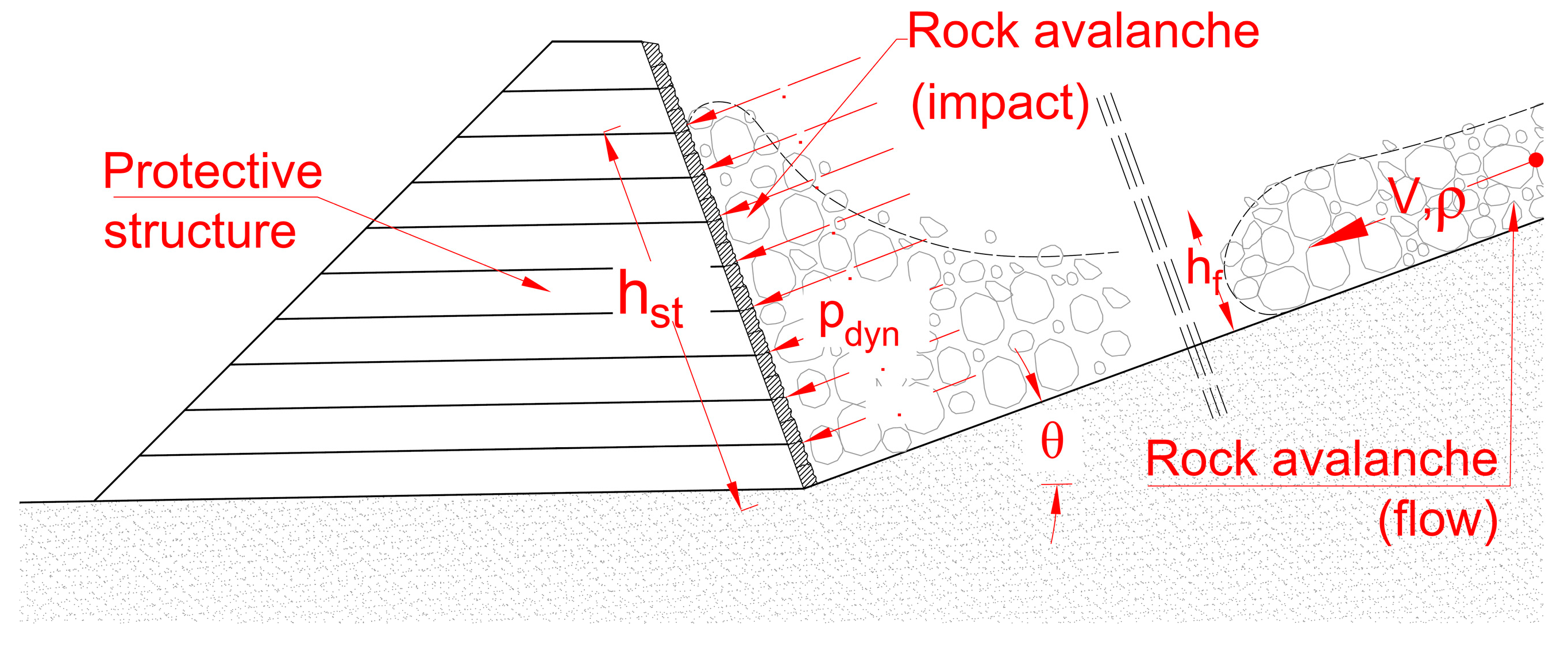
According to [6,7] (Austrian Standard—ONR), the impact can be calculated using Equations (3) and (4). The equation proposed by Ashwood and Hungr in [23], represented by Equation (5), shows an analogous design approach, with the dynamic and static impact pressure (pdyn, pstat), the dynamic and static impact force (Fdyn, Fstat), the static deposition height (hst), the impact width (b), and the density (). The velocity (v) and flow depth (hf) refer to the granular mass just before it hits a protective structure. Thus, in Equations (1)–(5), the granular mass parameters (v, , and hf) are used to determine the impact on a protective structure (Figure 1).
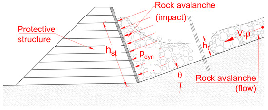
Figure 1.
Schematic illustration of the determination of the impact of a rock avalanche on a dam.
A comparison of Equation (1) with Equation (3) shows that a dimensionless empirical factor, i.e., the earth pressure coefficient (K), is considered for the calculation of the static action. The same applies to Equations (2), (4), and (5), where the factor () is taken into account as a dimensionless empirical parameter to determine the dynamic impact (Fdyn) on the protective structure. In the following, the maximum values of dynamic pressure and dynamic force are denoted as (ppeak) and (Fpeak).
There are hardly any available data sets on the effects of rock avalanches on protective structures, and such data sets are used to determine the earth pressure coefficient (K) and the factor . Monitoring an impact on a real structure, especially in regard to rock avalanches, is difficult to do and usually fails due to the large dimensions of such processes. In many cases, the estimation is based on numerical simulations or on the back-calculations of real events. The numerical simulations of the runout areas of real events can be explained geometrically with real events based on the deposition figures. An efficient and economical way to determine the factors K and lies in the execution of model tests. In the following sections, different model experiments are briefly listed, and the experimental setup of the University of Innsbruck is described. The dimensionless dynamic coefficient () is first determined directly from the experimental results and compared for plausibility with real events. Subsequently, the experimental results and the results of the DEM simulation are scaled and compared. A continuum mechanical consideration of the scaling and design of landslides and debris-flow experiments can be taken from [24].
2. Model Tests for the Investigation of Dry Gravitational Mass Movements
2.1. Overview of Existing Model Tests
Table 1 shows an overview of model tests of dry gravitational mass movements. The model tests generally describe geometrically simple shapes with flat surfaces and constant inclinations. A definition of the geometric boundary condition does not have to correspond to the exact geometric situations of real events. Rather, velocities (v) and flow heights (hf) must be generated in the model test, which can also occur realistically when scaled to real events. Thus, there is a possibility along the flume base, shortly before the impact on the barrier, to change the mass flow in such a way that larger flow heights (hf) can be produced [25].

Table 1.
Examples of model tests performed to study gravitational mass movements.
2.2. Model Test for This Work
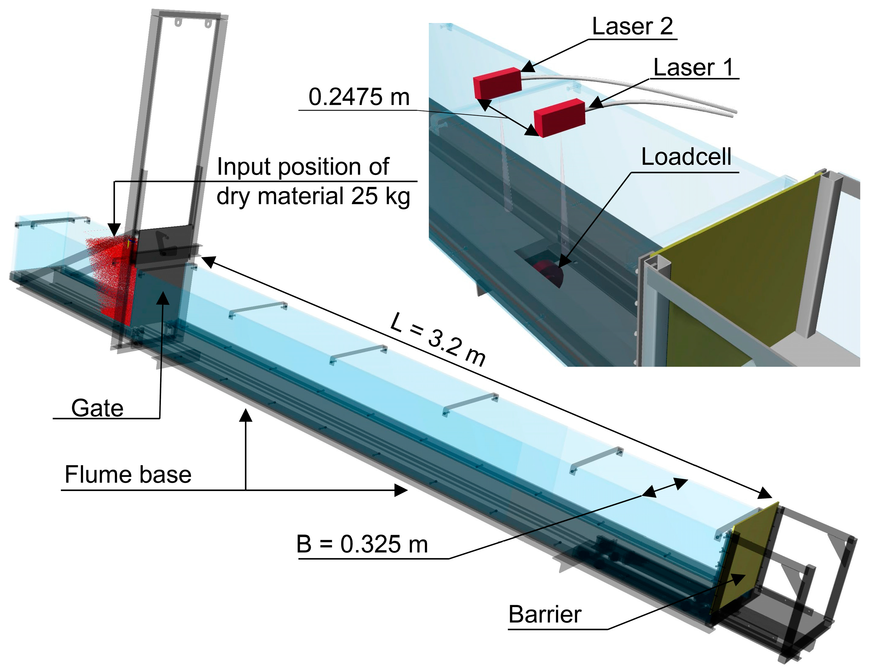
The model apparatus used for this work is located at the University of Innsbruck and consists of a reservoir, a gate, a flume base made of steel, sidewalls made of acrylic glass, and a rigid barrier made of steel (see Figure 2). The length of the flume base is about 3.2 m, and the width is 32.5 cm. In total, 91 model tests were carried out in 2020 and 2021 to investigate the effects on rigid barriers. Eighty-six tests were carried out with four different test materials (sand, a mixture consisting of sand and gravel, steel spheres, and glass spheres). Five tests were performed with corroded steel spheres to study the influence of surface roughness. All experiments were performed with dry material. The experimental procedure includes filling the reservoir with 25 kg of test material and opening the gate. The flowing movement and the impact on the rigid barrier were measured. The setup of the model test is shown in Figure 2. Model tests were carried out with inclinations (θ) of approximately 20° to 40°.

Figure 2.
Structure of the model experiment at the University of Innsbruck.
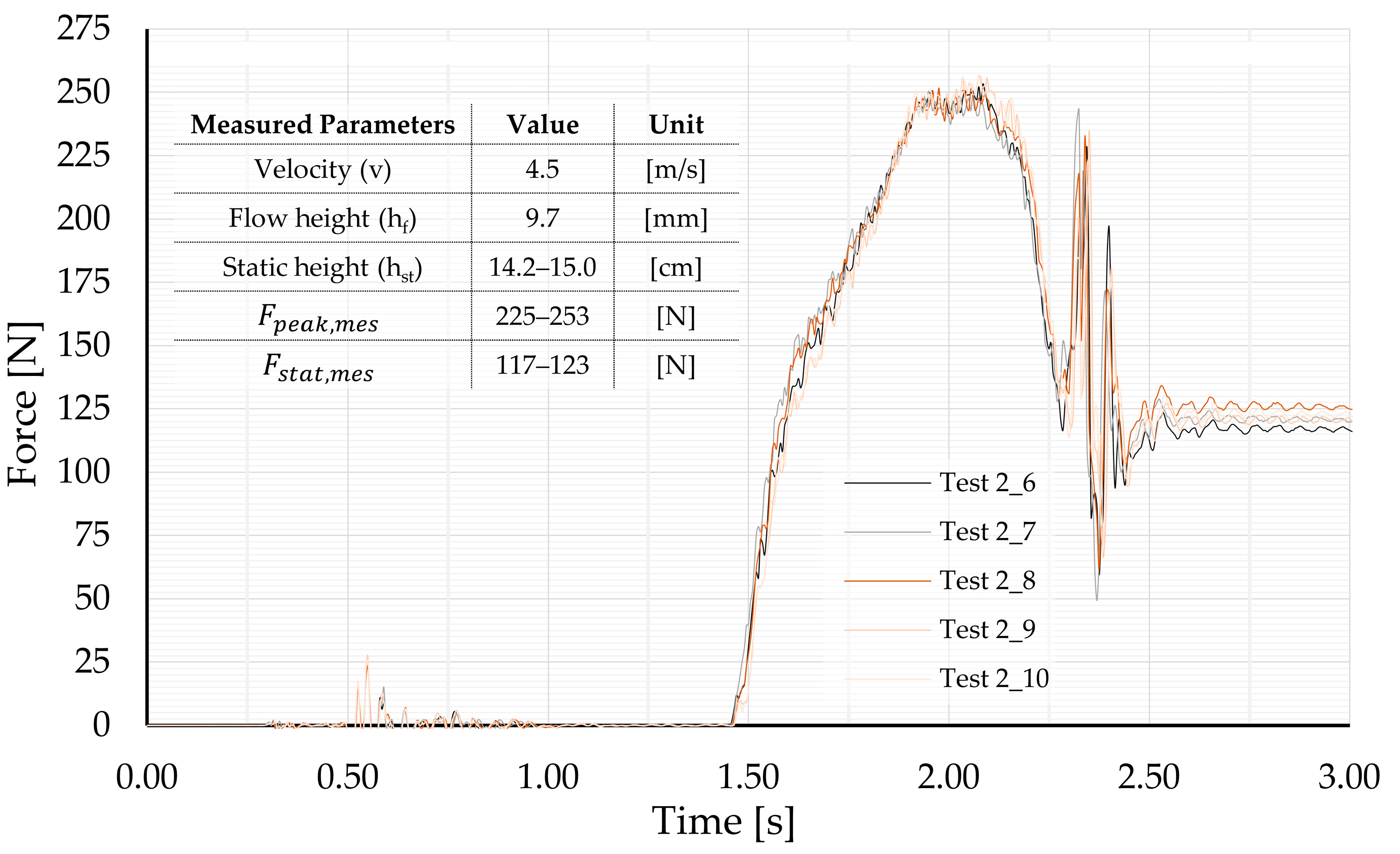
By opening the gate, the test material accelerates along the flume base and is stopped at the end by the rigid barrier. The measurement equipment included two optical distance lasers (Baumer OM70-L0600.HV0350) and a load cell (HBM U10M/1.25KN). The measurement enabled the determination of the flow heights (hf) and the velocity (v) of the granular mass with the help of the two optical distance lasers. The recording of the distance lasers and the load cell was synchronized by the measurement amplifier (Quantum MX840) with a measurement rate of 4800 Hz. The height (hst) was determined directly at the barrier using the grid (5 mm) on the acrylic glass pane. In addition, the recording was made with the help of two video cameras (SONY α6400L), so that the velocity (v) could be matched with the laser data. The videos were recorded with 100 fps and a resolution of 1020 × 720 px. Video analysis was performed using Kinovea® software. The front of the mass movement was marked frame by frame in the software. As a result, a distance-time history was obtained, from which the velocity could be determined. Figure 3 shows the results of the impact in the force–time history of a series of tests. Several test runs with the same boundary conditions (same material, same inclinations) were combined into one test series. The test boundary conditions of the results shown in Figure 3 are shown in Table 2.
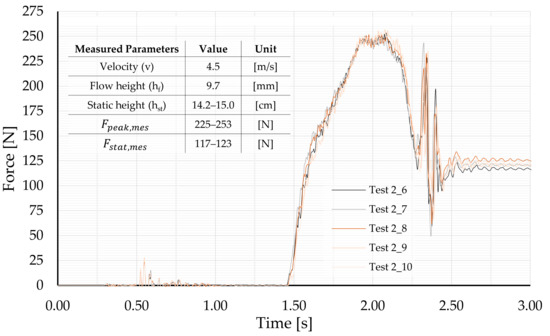
Figure 3.
Force–time plot on the rigid barrier for the test series according to Table 2 with the mean values of the measured flow velocity (v) and flow height (hf) and the upper and lower measured values of the dynamic and static impact force (Fpeak,mes, Fstat,mes).
Table 2.
Parameters of the test boundary conditions of the measurement results shown in Figure 3.
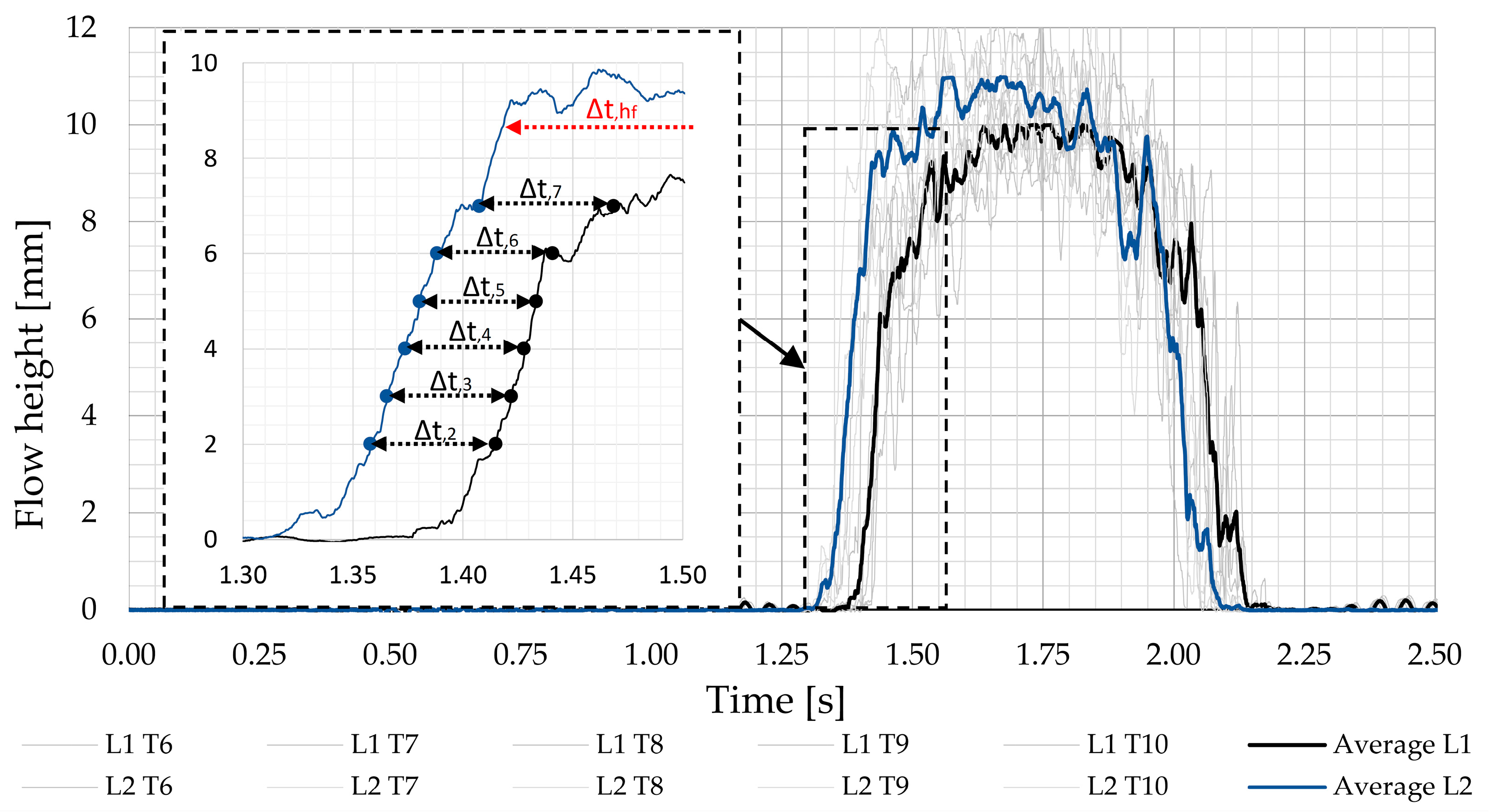
The results of the optical distance lasers of this test series, which recorded the measurements of the flow heights (hf) over time, are shown in Figure 4. In Figure 4, L1 denotes the measurement data of Laser 1, L2 denotes the measurement data of Laser 2, and, for example, T6 denotes Test 6. The individual measurement data of Laser 1 and Laser 2 are averaged and denoted as “Average L1” and “Average L2”. As shown in Figure 4 on the right, the time difference can be determined by comparing identical flow heights (∆t,2 to ∆t,7). With the distance between the two lasers of 24.75 cm, the velocity (v) can be determined. The median value of the velocities (v) from the interpolation of the flow heights (hf) between 2 and 7 mm by using the time difference (∆t,2 to ∆t,7) is 4.45 m/s. An interpretation of the median yields a velocity (v) of approximately 4.47 m/s. Since the interpretation of the velocity (v) is strongly influenced by constant flow heights, due to the horizontal plateau, the specification of the velocity (v) to two digits after the decimal point is not justified. In addition, it must be taken into account that the velocity of the individual particles within the granular mass is not homogeneous. Thus, the velocity (v) is interpreted as sufficiently accurate to 4.5 m/s. In Figure 4, ∆t,hf shows that the determination of the velocity (v) does not work for constant flow heights (hf).
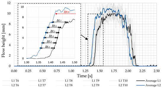
Figure 4.
Test results of the flow height (hf), measured with Laser 1 (L1) and Laser 2 (L2) for Tests 6 (T6) to 10 (T10). The mean value of all test results is denoted by Average L1 and Average L2. ∆t,2 to ∆t,7 denotes the time difference at the same flow height between Average L1 and Average L2.
With the help of the measurement results, the empirical factor (α) and the earth pressure coefficient (K) of Equations (3)–(5) can be determined. For the test series of Table 2 and the results of Figure 3, the empirical factor (α) is obtained from the maximum impact (Fpeak,mes) for the test material of steel spheres and a flume base inclination (θ) of 30.2°:
The empirical factor () can then be used to determine the actions of real events of steel spheres. Actions based on model tests with steel spheres do not describe natural events. Model tests with ideal grain shapes have several advantages. The test results with an almost perfect geometric spherical shape, such as that of the steel spheres, must always produce analogous test results and are, thus, a quality characteristic for a model test and the measuring instrumentation used. Due to the geometric spherical shape and the smooth surface, the rolling resistance of the individual particles can be almost neglected. Furthermore, due to the high density, steel spheres can also be used to derive statements about the influence of density on the test results. Due to the small measurement differences for repetitive tests, the test series with steel balls is well suited for the analysis of scale effects.
In addition to the direct determination of the empirical factor (α) in Equation (6), it is possible to introduce further dimensionless parameters to describe it. With the help of Edgar Buckingham’s developed principle [30], it is possible to determine dimensionless parameters from dimensionally significant quantities (e.g., velocity (v)). In the literature, the procedure is called Buckingham’s π theorem [30,31,32,33,34]. The following shows how dimensionless parameters can be determined. The dimensionless quantities used in Buckingham’s π theorem must be relevant for the physical process. If many physical quantities are chosen, a large number of dimensionless arguments must be introduced. If too few physical quantities are chosen, the similarity is not sufficiently defined [32].
2.3. Buckingham’s π Theorems and the Determination of Dimensionless Parameters
If dimensionless empirical factors, such as α in Equations (2), (4), and (5), are determined from model experiments, the question of what dependence they exhibit and how they can be determined remains open. One possibility in the determination of dimensionless factors is the application of Buckingham’s π theorem. If, by analogy to Equations (2), (4), and (5), the maximum dynamic impact (Fpeak) is sought as a function (f) depending on gravity (g), velocity (v), the width of the impact (b), flow height (hf), and density (), the following dependence is obtained:
The conversation of the dimensionally influenced parameters from Equation (7) into dimensionless terms is only possible if each basic dimension occurs in at least two dimensionally influenced parameters. According to [30] or [34] we let Π represents a dimensionless product of the form:
If, instead of the parameters Fpeak, g, v, b, hf, and , the corresponding units are used, it follows that
which can be transformed to
Since the sum of the exponents () for the units kg, m, and s must vanish, Equation (10) becomes
This results in 6 unknown exponents ( and 3 equations (Equations (11–13)). This leaves 3 degrees of freedom. One possibility is to assume that are determinable from the remaining parameters . This results in the following dependencies:
Substituting Equations (14)–(16) into Equation (8) yields
By transforming, one obtains afterward
The terms determined in this way within the brackets are dimensionless and can be considered as possible key indicators.
The independent exponents , and of Equation (18) can be freely chosen. The term inside the bracket remains dimensionless. As an example, we assume , . From these follows:
The analogous dimensionless parameters can be determined by adding further parameters to Equation (7), and the dependent and independent exponents can then be determined. Consequently, if the objective is to determine the maximum dynamic impact (Fpeak) on a protective structure due to granular mass movements using Equations (2), (4), and (5), whether the dimensionless parameters in Equations (19)–(21) are suitable to describe the factor α of Equations (2), (4), and (5) can also be checked. The dimensionless parameter of Equation (19) cannot be used because it already contains the unknown of the maximum dynamic impact (Fpeak). The dimensionless parameter of Equation (20) proves to be rather unsuitable in its simplicity. Based on the results of the model tests, whether the dimensionless parameter of Equation (21) is suitable to determine α is checked.
Using linear regression of the measured test results, the constant factor (X) in Equation (22) can be determined, which gives the smallest deviation between Fpeak,mes and Fpeak,calc. Here, Fpeak,mes denotes the maximum, dynamic measured impact on the barrier. Fpeak,calc denotes the maximum, dynamic calculated impact. Fpeak,calc is determined using the measured velocity (v), the bulk density (), the width (b), and the flow height (hf) analogous to Equation (4).
In contrast to Equation (6), which only takes into account the data from the steel spheres at a flume base inclination (θ) of 30.2°, the linear regression considers all 86 test results. If the 86 test results of the model test are analyzed in this way, the statistical characteristics shown in Table 3 are obtained.
Table 3.
Statistical characteristics of linear regression for testing factor α using the 86 experimental results and Equation (23).
Table 3.
Statistical characteristics of linear regression for testing factor α using the 86 experimental results and Equation (23).
| Statistical Parameters | Value | Description |
|---|---|---|
| Analyzed values | 86 | Number of model tests for the analysis of Fpeak,mes |
| Coefficient of determination | 0.93 | - |
| Intersection/Constraint point | 0/0 | [N] results in a Froude number Fr = 0 [–] |
| Coefficient X | 9.89 | |
| 2.5% Quantile of X | 9.31 | |
| 97.5% Quantile of X | 10.46 |
The coefficient of determination of 0.93 indicates that the empirical parameter with the choice of is well suited to determine the maximum dynamic impact Fpeak. The values of the action on the rigid barrier Fpeak,mes and Fpeak,calc are shown in Figure 5. Furthermore, the deviations between Fpeak,mes and Fpeak,calc are shown in percentages. All deviations in Figure 5 are shown positively on a logarithmic scale. The analysis of the deviation of the 86 model tests with different inclinations (θ) and different test materials (sand, mixture, glass, and steel) shows that the calculated impact force (Fpeak_calc, Table 3, Equation (24)) is approximately 54% below and 46% above the measured impact force (Fpeak_mes). Figure 5 shows for Froude numbers (Fr) higher than 10 a maximum deviation of 57%. For Froude numbers (Fr) lower than 10 the maximum deviation is approximately 1050%. The representation in Figure 5 indicates that the deviations between Fpeak_mes and Fpeak_calc calculated with Equation (24) are large (especially for small forces). This is because the deviations are presented as relative (%) and not with absolute values. The median of the deviations using Equation (24) of all 86 test results is 23.4%. The smaller the Froude number (Fr), the greater the deviations between Fpeak_mes and Fpeak_calc. Since no data are available for Froude numbers lower than 6, whether this trend will continue cannot be determined. The determination of the factor is therefore limited to Froude numbers between 6 and 20 and to the test material investigated (sand, gravel, glass, and steel).
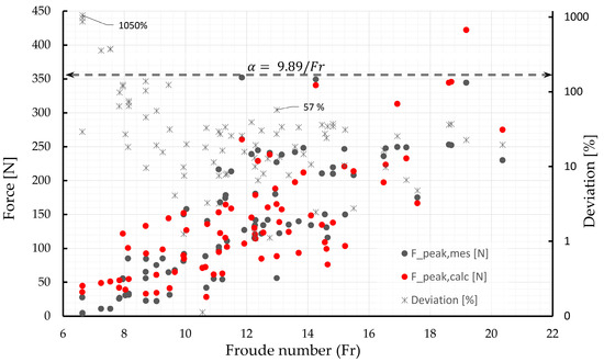
Figure 5.
Comparison of the measured maximum impact force Fpeak,mes with the calculated impact force Fpeak,calc according to Equation (24) and the deviation between Fpeak,mes and Fpeak,calc. Result of the factor by analyzing different ranges of the Froude number using linear regression.
If the test results for Fr < 10 and Fr > 10 are considered separately, different results are concluded. If the linear regression is limited for a Froude number higher than 10, the parameter , and the coefficient of determination is 0.95 (see Figure 5). For a Froude number lower than 10, the parameter , and the coefficient of determination is 0.85 (see Figure 5). This evaluation includes the interpretation of all test materials. If only natural grain shapes (sand and mixture) are considered, independent of the Froude number, the result is with a coefficient of determination of 0.88. It is clear from the different observations that the determination of an empirical factor also depends on the interpretation of the observer.
If the results of these model tests serve as the basis for a design concept, both dimensional analysis and a corresponding model law must be considered. Interpretations of dimensionally affected measured values cannot be universally scaled with the help of a uniform geometric scale factor).
3. Dimensional Analysis
3.1. Base Quantities
Dimensional analysis is a mathematical tool to determine the similarity between model tests and real events. In the following, real events are referred to as prototypes. Physical parameters have units and depend on different base quantities. These base quantities are the basis for all physical parameters. A basic quantity may never be dependent on another basic quantity. Subsequently, derived quantities can arise from basic quantities. Thus, base quantities are defined in the following, with which all further physical quantities can be described. The composition of the basic quantities is called the basic quantity system. The most important basic quantities in connection with the determination of the effects of gravitational mass processes are described by the geometric quantity (L), mass (M), and time (T). Other basic quantities in the SI system, such as the temperature (T) or the amount of substance (n), are not considered concerning the problem at hand. The defined basic quantities can be put together in such a way that no quantity is dependent on the other. This results in the following basic quantity system:
- Length–Mass–Time [L-M-T].
Concerning the determination of the impacts on protective structures, the following relevant parameters can be generated based on the basic quantities according to Equations (1)–(5). Physical quantities of the model test that depend on the three basic quantities are listed in Table 4.
Table 4.
Physical parameters regarding the determination of gravitational mass movement effects.
3.2. Similarity Laws
Model tests are mostly geometrically reduced replicas of a real process taking place in nature. When mapping from the model to a prototype, the consideration of geometric, kinematic, and dynamic similarities is required [35].
3.2.1. Geometric Similarity
Geometric similarity exists when all geometric dimensions (length, width, height, roughness of the substrate, and grain diameter) are reduced by the same scale factor (λL). The scale factor is also called the model scale. The application limits of the geometric similarity become apparent in the case of the roughness of the subsurface. The roughness can be reduced by the model scale, but a change in the flow behavior is conceivable [36].
3.2.2. Dynamic Similarity
A model is dynamically similar if all acting forces are reduced by the same scale factor. Gravity, inertia, and friction represent some examples of the acting forces in a process. These must be scaled by the identical factor to gain dynamic similarity [36].
3.2.3. Kinematic Similarity
A time-dependent process is kinematically similar if the parameters changing over time are reduced by the same model factor. For example, the velocity or acceleration of a mass represents a time-dependent process:
3.3. Model Laws 1 G
The influence of gravity (g) is of elementary importance for model experiments. For most engineering problems, the choice of gravity (g) as a constant with g = 9.81 m/s2 is sufficient.
The effective vertical stresses in the soil are determined according to Equation (28). Gravity has an influence on the determination of the stresses. If test values are scaled from the model to a prototype, the gravity must also be multiplied by a scale factor λG. However, this remains constant for both systems, the model test, and the prototype. The dynamic similarity of the model is thus not completely given. Such model tests are called 1-g model tests [37]. In order to keep the similarity of gravity, centrifuge models are used [38]. For the compliance with this model, the following law must hold:
If a geometric similarity is further required, the condition from Equation (25) also applies. The following is then valid:
It follows from this that
Analogously, a derivation of further scale factors for different physical quantities is possible (Table 5).
Table 5.
List of scale factors based on the 1-g model law and Froude’s model law.
3.4. Froude’s Model Law
Froude’s model law is mostly used in hydraulic engineering experiments. Here, the Froude number (Fr) in Equation (32) describes the ratio of inertial force to gravity. The Froude number (Fr) is thus a function of velocity (v), gravity (g), and characteristic length or height. In an open channel, the flow height (hf) describes the characteristic height of the fluid. The Froude number (Fr) is dimensionless:
According to Froude’s model law, the flow state (subcritical or supercritical flow) of fluid must remain the same for the model test and the prototype. In hydraulic engineering, a value of Fr < 1 distinguishes a subcritical flow state, and a value of Fr > 1 indicates a supercritical flow state. The scale factor of the velocity ) for Froude’s model law can be derived by [36]. The following requirement must hold for Froude’s model law. From the requirement that furthermore a geometrical similarity (Equation (25)) and the relation of gravity (Equation (29)) remains, it follows that
By transforming, one obtains the scale factor of the velocity ( as a function of the geometric scale factor ):
According to Equation (33), it is required that the Froude numbers (Fr) are identical in both the model test and the prototype. According to [36], this applies in particular to the distinction of the flow condition. That is, interpretations or the determination of empirical parameters in the range of the Froude number Fr = 1 are to be critically evaluated. Limitations of Froude’s model law, especially with respect to hydraulic engineering experiments, can be found in [36].
3.5. Scale Factor of the Mass and the Force
Further scale factors based on the 1-g model law or Froude’s model law, e.g., for the mass (λm) or the force (λF), can be determined by comparing dimensionless parameters. The dimensionless parameters can be calculated using the Buckingham theorem as shown:
Thus, the dimensionless factor from Equation (35), with the help of the geometric scale factor ) of Equation (25) and the scale factor of density to the scale factor of the mass (), leads to the following:
The scale factor of the force ( can be determined analogously and can be found in [39]. Table 5 shows the most important scale factors () in the investigation of gravitational mass movements with the aid of model experiments.
The 1-g model law and Froude’s model law (also comparing Equation (31) with Equation (34)) follow the same scale factors () for further physical quantities. The scale factors given in Table 5 are related to the geometric scale factor (. This makes it easier to interpret the scale value of the scale factor.
4. Scaling of the Model Test for This Work
Based on the similarity laws and the 1-g model law as well as Froude’s model law, it has been shown that all scale factors can be represented as a function of the geometric scale factor (Table 5). This should be applied to all process parameters to scale from the model test to the prototype. Froude’s model law further limits the application of scaling. The Froude number (Fr) in the model test and the prototype should not differ. This is especially true for the subcritical flow states (Fr > 1) and the supercritical flow state (Fr < 1). For the investigation of effects due to granular mass movements with the aid of model tests, Froude numbers in the prototype are analyzed below. Since the design approaches according to [6,7] refer to debris-flow processes, the velocities (v) and flow heights (hf) of debris flows and rock avalanches are listed in Table 6.
Table 6.
Velocity (v), flow heights (hf), and Froude numbers (Fr) of debris flows and rock avalanches published in [40,41,42,43,44,45,46,47,48,49,50,51,52,53,54,55,56,57,58,59,60,61,62] by different authors.
The determination of velocities (v) and flow heights (hf) as well as the resulting Froude numbers (Fr) are based partly on observations (estimated or measured) and partly on back-calculations. Thus, the velocities (v) and flow heights (hf) of the Alpl rock avalanche given in Table 6 are obtained from the mean values of Cross Section 1, Section 2, Section 3, Section 4 and Section 5. Table 6 shows that debris flows generally reach smaller velocities (v) than rock avalanches. Data on flow heights (hf) of rock avalanches are hardly documented. Flow depths at Piz Cengalo were not measured directly at the process but were determined using numerical back-calculation. Although debris flows generally have low frictional resistance to flow due to the complete water saturation of the material, they hardly reach the flow velocities (v) that are reached in rock avalanches. From the authors’ point of view, the following main factors distinguish the two processes.
Rock avalanches usually break loose on steep walls. The transformation of the potential energy into kinetic energy takes place in a very short time, because the almost vertical walls offer hardly any resistance to the fall. Due to the large mass movements of rock avalanches, usually several 10,000 m3, they can be less well channeled geometrically. In contrast, debris flows usually follow confined channel cross sections. Consequently, an increase in the flow rate of debris flows also increases the flow height (hf). Therefore, in regard to rock and landslides, lower flow heights (hf) result in higher velocities (v), compared to debris flows. This also results in higher Froude numbers (Fr) for rock avalanches compared to debris flows.
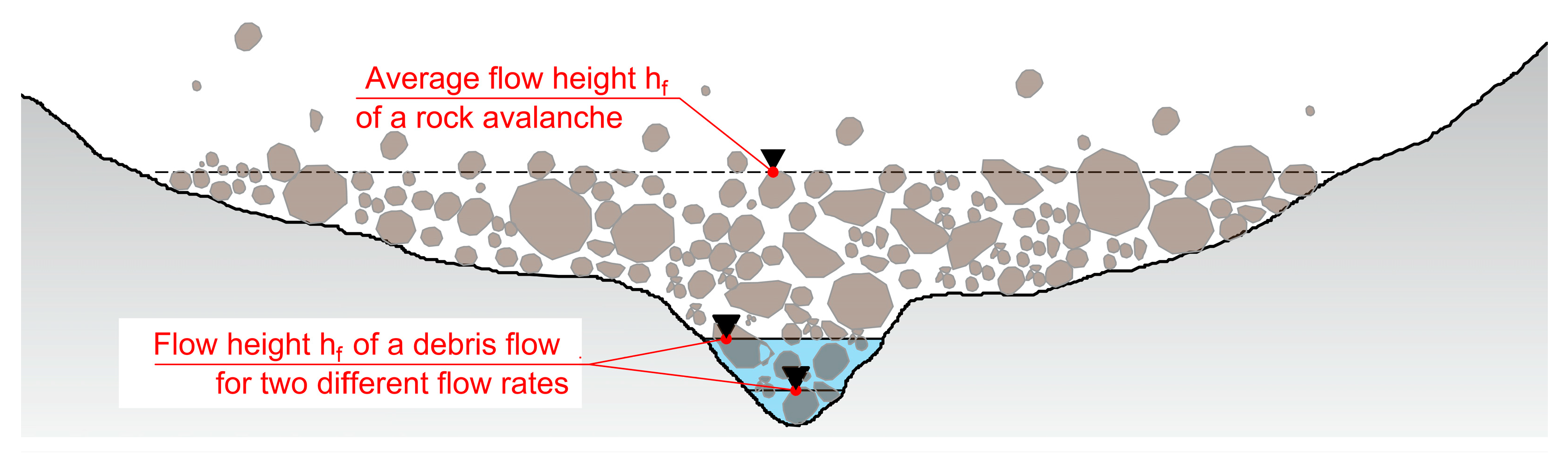
Figure 6 shows a cross section of two possible gravitational mass movements, debris flow and a rock avalanche, which represents the authors’ considerations. It is shown that due to the strong supercritical flow of rock avalanches, a fixed value of the flow depth (hf) is difficult to determine.
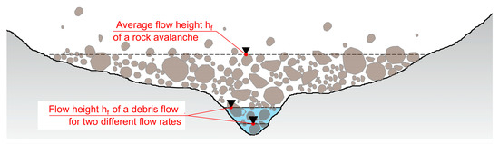
Figure 6.
Cross section with flow height through a possible debris flow and rock avalanche.
An analogous behavior can be established by considering snow avalanches. For example, as described in [63], large faster snow avalanches move in a supercritical regime with Froude numbers of about 2–6. Froude numbers between 6 and 15 are achieved by dilution avalanches. Since the geometrical situation in the transverse and longitudinal direction is not constant, it follows that debris flows and rock avalanches cannot be represented by a single Froude number that remains constant over the entire process duration. In [63], the Froude number during the whole process is shown. Froude numbers from 0 to approximately 15 are reached. Since the focus is on determining the effects of rock avalanches on protective structures, the following considerations are used to define ranges of realistic Froude numbers:
- Protective dams are usually built on a slope inclination of up to 35° for design purposes. This rather “flat” slope has a greater resistance compared to steep rock faces. It follows that the velocity at the time of impact is smaller than the maximum observed velocities in Table 6.
- Protective structures against rock avalanches in narrow valley cross sections are unsuitable because large mass movements quickly backfill a protective structure, and the shooting mass immediately fills the uphill terrain.
- Protective dams are usually designed as linear structures. The length of the dams allows a strong lateral deflection of the mass. This results in considerably lower flow heights (hf).
- Typical construction heights of protective dams reach approximately 25–30 m and are built where the rock avalanche does not reach the flow depth (hf), which can “run up” the dam crest.
- The block sizes occurring in rock avalanches usually reach several meters, so the flow height should be assumed to be hf > 1–2 m based on the block size alone.
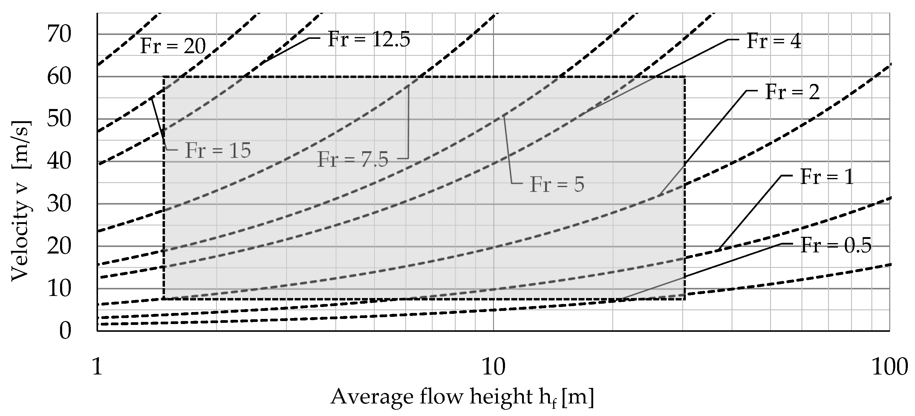
Based on the above considerations of velocities and flow heights, in Figure 7, possible areas for rock avalanches can be defined. The range shown in Figure 7 assumes that the rock avalanche can be stopped by a protective structure. This realistic Froude numbers (Fr) refers immediately before a protective structure is impacted.
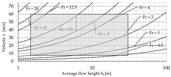
Figure 7.
Possible area (shaded) of Froude numbers (Fr) due to rock avalanches before a protective structure is impacted.
5. DEM Simulation of the Model Test for This Work
The calculation of the force–time history of the impact on the rigid barrier was performed with the Rocky® software from ESSS (Houston, TX, USA) using the Discrete Element Method (DEM). The comparative calculation referred exclusively to the test series with steel spheres (2 mm) under an inclination of the flume base θ = 30.2°. Based on the DEM simulation, in addition to the force–time history, the velocity (v) and flow height (hf) of the granular mass before impacting the rigid barrier were determined. For the description of the interaction between the particles or between the particles and the model, “Normal Force” using a linear spring dashpot model and “Tangential Force” using a linear spring model with the Coulomb limit were considered in the numerical DEM simulation. In the DEM simulation, the friction and restitution coefficients in Table 7 were considered. The model parameters in the DEM simulation were calibrated with the test results and determined based on the laboratory tests performed. The model parameters used in the calculation are shown in Table 7. The round particles in the DEM model were filled through an “inlet” above the gate (see Figure 8a). In total, about 760,000 particles with a diameter of 2 mm and a total weight of 25 kg were created.
Table 7.
Friction and restitution coefficients between the particle and particle model test used for DEM simulation. The column on the right describes the results of the laboratory test for the test material.
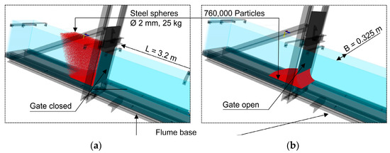
Figure 8.
DEM model; the creation of the particles (a) and the opening of the gate (b).
When the flap was opened (Figure 8b), the particles accelerated along the flume base until, after approximately 1.1 s, the first particles reached the rigid barrier.
Figure 9 shows a comparison of the force–time curve of the action on the rigid barrier using the measured test data and the calculation results of the DEM model. The maximum dynamic force (Fpeak) and the load duration achieve very high qualitative agreement (see Table 8). The quantitative deviations are shown in Table 8. In addition to the force–time curve, the duration between the opening of the gate and the impact of the particles on the barrier are also shown in Figure 9. The opening of the gate occurred after approximately 0.5 s. The first particles reached the barrier after approximately 1.2 s. The total impact time on the rigid barrier was approximately 1.0 s. The impact on the rigid barrier caused some particles to shoot upwards along the barrier. The additional impact on the rigid barrier of these particles resulted in a double peak in the force–time history. Both the measured experimental data and the DEM model show this (see Figure 9).
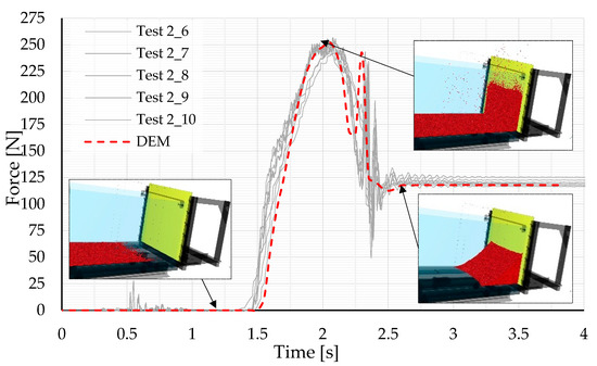
Figure 9.
Comparison of the test results of the force–time history on the rigid barrier with the calculation results of the DEM simulation.
Table 8.
Comparison of the measured experimental results with the calculated values of the simulation results. For definitions of the parameters Fdyn, Fstat, v, and hf, see text.
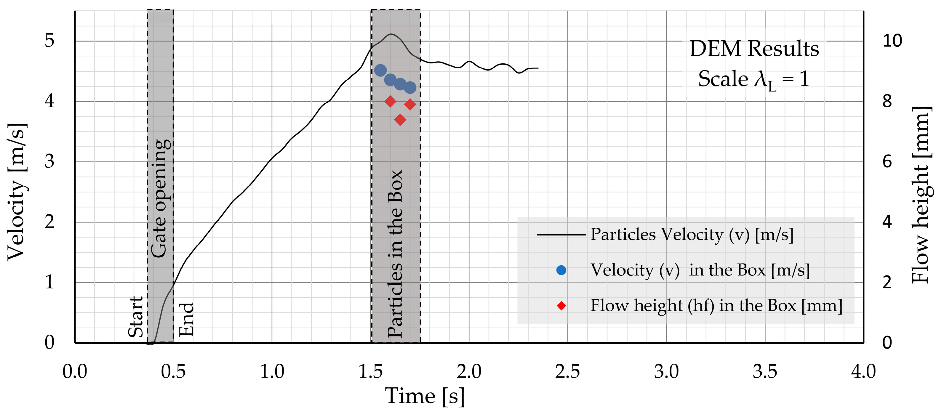
Figure 10 shows the analysis of the particle velocity from the numerical DEM simulation. If all individual particle velocities are calculated, the maximum value of the velocity of a particle can be represented as a function of time. This means that for a fixed point in time, all velocities of the 760,000 particles were calculated, and the maximum value of the particle was then plotted. This function is called “Particle Velocity (v)” in Figure 10 and shows the course of the maximum “Particle Velocity (v)” over the entire test run. Since the determination of the velocity is thus independent of the location of the particle, these calculation results must be considered as an upper limit. The velocity was therefore determined based on a defined location “Box”. The “Box” is located approx. 0.25 m in front of the barrier, because rebounding particles falsify the results. The blue points in Figure 10 represent the mean value of the velocity of all particles which are inside the “Box”. The red points in Figure 10 represent the maximum flow height (hf) of all particles which are inside the “Box”. The values “Velocity (v) in the Box” and “Flow height (hf) in the Box” in Figure 10 are therefore the values which can be used for the comparison with the test results.
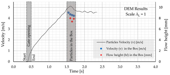
Figure 10.
DEM results of velocity (v) and flow height (hf) (see text for definitions).
Table 8 compares the measured test results with the calculated values from the DEM simulation and determines the deviations. Except for the flow height (hf) and the static deposition height (hst), the deviations between the measured values and the calculated simulation results are less than 2%. The measured values of the flow height (hf) of the granular mass are about 17% higher than the calculated value. If the range of flow heights (hf) of Laser 1, which is closer to the rigid barrier, is considered, the calculated value is within the experimental results. Flow heights between 7.3 and 12.0 mm were measured for Laser 1. The mean static deposition height (hst) in the DEM model is about 6.8% higher than that measured in the tests.
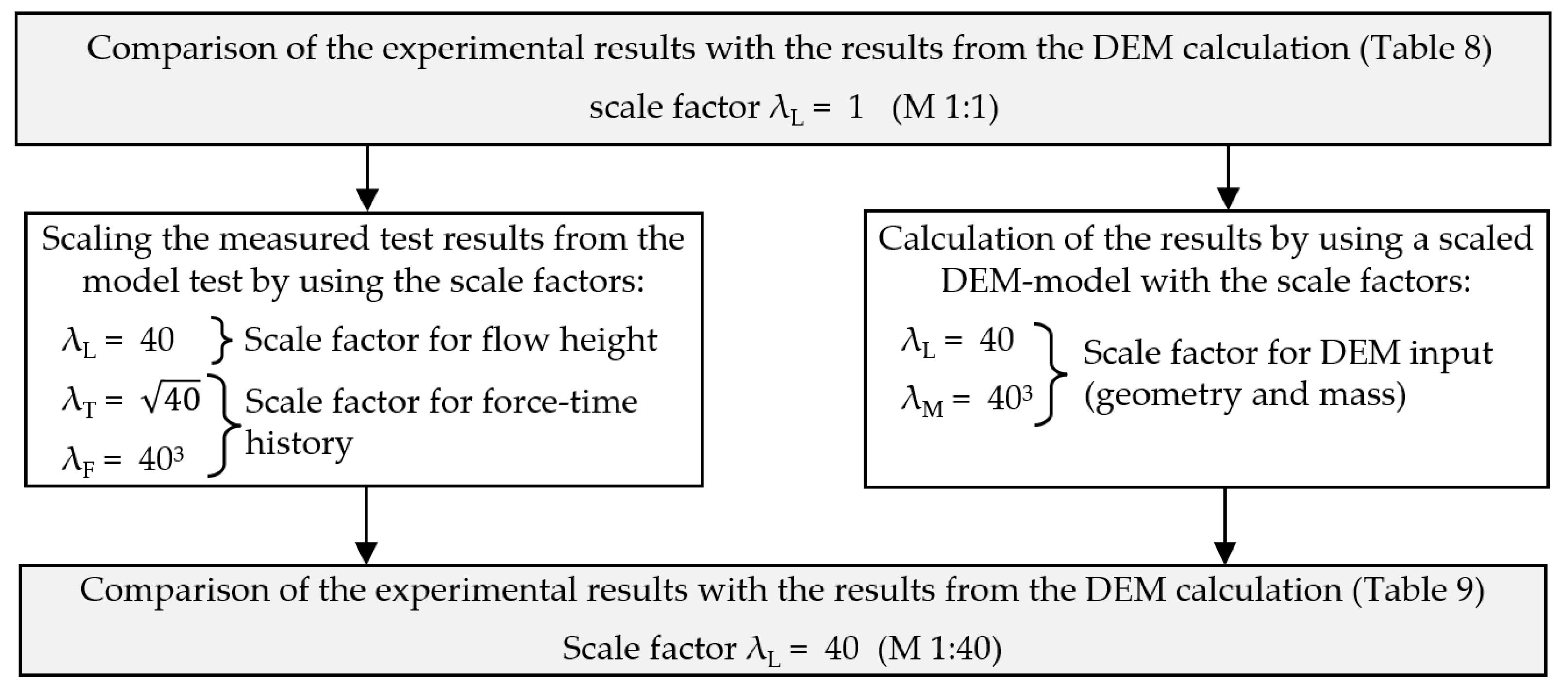
With the aid of the defined scale factors (), it is possible to scale the parameters from the model test to the prototype. For a comparison of the scaled measured values with a scaled DEM model, a fixed scale factor () was taken into account. In [26], a possible geometric scale of 1:30 to 1:50 was identified for the model test. If a geometric scale factor of 40 is selected, the values of Table 9 are obtained. The measured results of the model test were calculated with the scale factors , and . The DEM model was scaled with the scale factors and . The concept of the comparison is shown in Figure 11.
Table 9.
Comparison of the parameters with the scale factor = 1 and = 40.
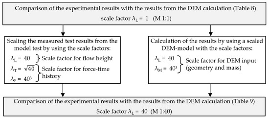
Figure 11.
Concept of the procedure for comparing the scaled results from the model test and the DEM model.
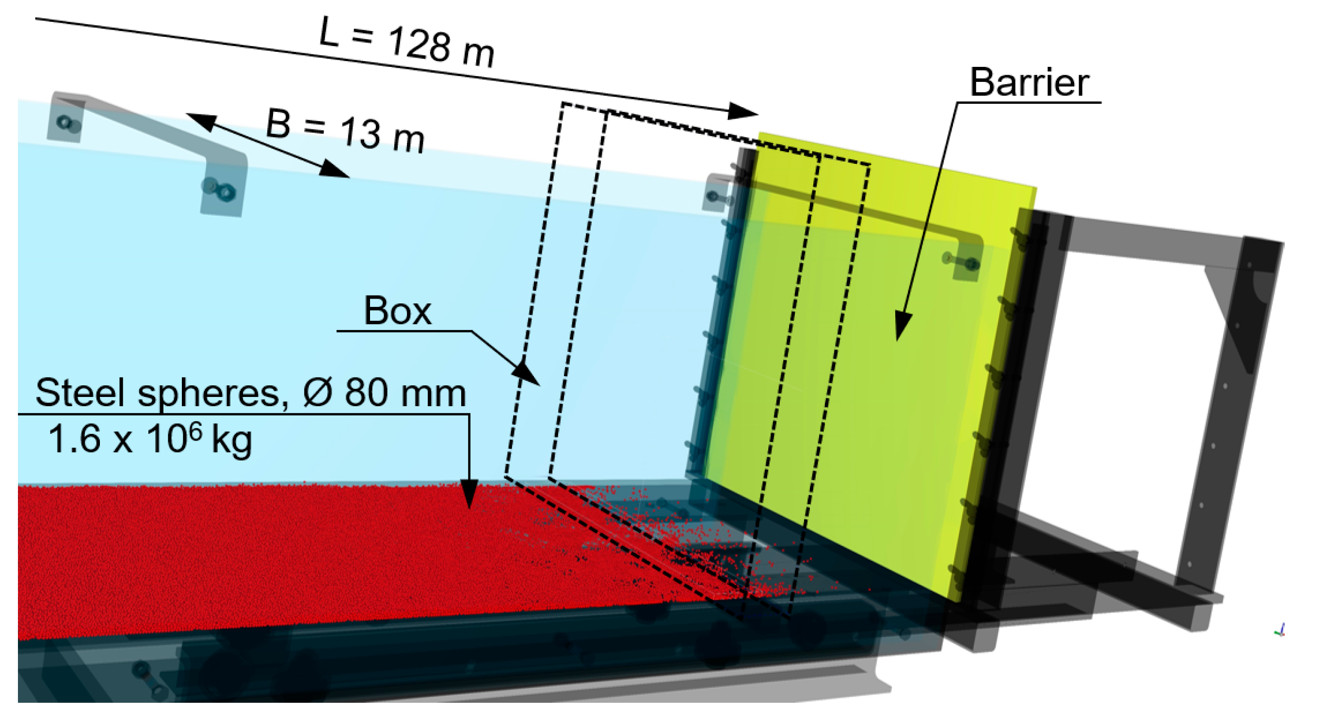
The test results of the model test according to Figure 3 were multiplied by the scale factors = = , and = 403 (Table 5 and Table 9). According to Figure 11, the comparison is performed with a scaled DEM model. The geometric dimensions of the model and the particles of this scaled DEM model is shown in Figure 12.

Figure 12.
Dimensions of the scaled DEM model with the geometric scale factor = 40, Geometric position of the “Box” for the analysis of particle velocities (v) and flow height (hf).
The comparison of these measured, scaled test results and the results from the scaled DEM model are shown in Figure 13.

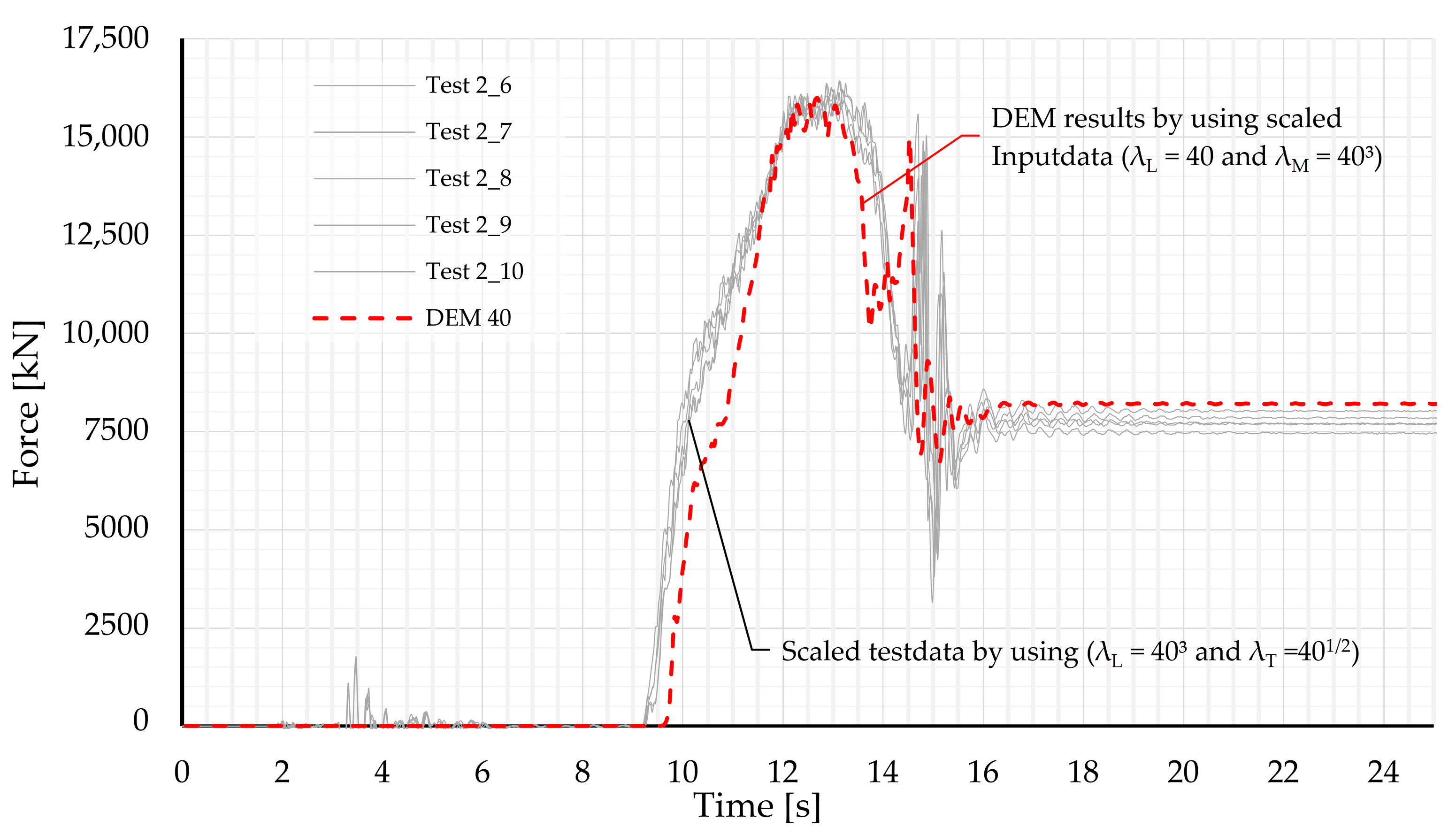
Figure 13.
Force–time history of the impact on the rigid barrier, a comparison of the scaled test data with λF and λT, and the calculated results of the scaled DEM simulation with λL and λM.
A scaled DEM model was used to calculate the impacts (Fpeak) and (Fstat), the flow height (hf), and the velocity (v). In the DEM model, all geometric quantities were scaled with the geometric factor = 40. The granular mass was enlarged by the factor . In Figure 12, the new boundary conditions of the scaled DEM model are shown. A comparison of the force–time history results using the scaling factors (λL, λF, and λT) and the experimental data (λL and λM) in the DEM model is shown in Figure 13. The evaluation of the flow velocity (v) and the flow height (hf) is presented analogously to Figure 10 for the scaled DEM model in Figure 14.
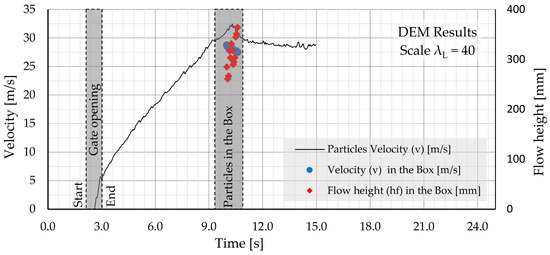
Figure 14.
Results of the scaled DEM model for velocity (v) and flow height (hf).
Figure 13 and Figure 14 as well as Table 10 show that the individual parameters from the scaled model results and the scaled DEM model still provide almost the same results. The largest deviation between the scaled model results and the scaled DEM simulation results, according to Table 10, is in the flow height (hf) with an amount of 11.1%. The difference between the maximum dynamic impact (Fpeak) is 1.1%, and the static impact (Fstat) is 6.5%. The evaluation of the particles inside the box (Figure 12) in the scaled DEM model results in a mean velocity (v) of 28.2 m/s. Thus, the velocity differs by 0.3 m/s when comparing the scaled DEM model to the measured scaled experimental results. The mean flow height (hf) in the DEM model is 345 mm, which is 43 mm lower than the measured scaled test results (Table 10). The static deposition height (hst) reaches 6403 mm in the scaled DEM model, which is about 9.3% higher than the scaled deposition height of the model test.
Table 10.
Comparison of the scaled model results with the results of the scaled DEM simulation.
6. Discussion
If the test data for determining the impacts on a rigid barrier are scaled using a model test with the model laws (1-g or Froude), an equivalent scaled numerical DEM model gives similar results. Regardless of whether the scale factor used was or , a deviation of a maximum of 6.5% was achieved for the static impact (Fstat). The maximum dynamic impact (Fpeak), which is decisive for the design, reaches a maximum deviation of 1.1%. The velocity (v) could be calculated with an accuracy of 1.1%. For the flow heights (hf), deviations of a maximum of 17% result, and these lie within the measuring range of Laser 1. The static deposition height (hst) in front of the barrier was overestimated in the DEM model, independently of the scale. A comparison of the deposition height (hst) was made using the mean values and amounts to a maximum of 9.3%.
With the help of numerical DEM simulation, it is shown that the model laws (1-g and Froude) are capable of scaling measured values from model tests. However, a scaling of the measured values must lie within a firmly defined range. This range is limited by the observed quantities of a real rock avalanche or its prototype. Within the range, the scale factor () must be applied to all process variables. The process parameters must then match those measured or observed at the prototype. Knowledge of real parameters (velocity (v), flow height (hf), densities (), grain shape, or grain size) of real rock avalanches is, therefore, essential. The numerical DEM simulations act in this case as a link between the model test and the prototype.
If dimensionless parameters are introduced, it is generally assumed that they are not changed by scaling. However, this general assumption is not always justified in this context. In a DEM simulation, the interaction is described, among other things, with the help of a coefficient of restitution. This can be determined, e.g., from a drop test (Table 7). This approach may be physically correct, but it must be assumed that particles of different sizes do not result in the same restitution factor. The observation that, for example, smaller blocks reach higher velocities (v) and jump heights is, among others, also described in [65]. According to [65], it is, however, possible to consider a velocity-dependent or a mass-dependent restitution coefficient. In the DEM simulation, this would be possible by defining different material parameters depending on the particle size. In regard to [65], a mass-dependent coefficient of restitution can be defined with Equation (37).
with Rn(scaled) as a scaled, mass-dependent restitution factor, the mass (M), and a mass-independent fixed-parameter B. Parameter B can be determined, for example, by a drop test with different particle masses. Because the restitution factor is dimensionless, the parameter B is expressed in kilograms. Other mass-dependent scaling equations for the material model used are also conceivable. Equation (37) shows a possible way to scale the restitution factor for different particle sizes. It must be noted that Equation (37) is based on single impact considerations. For rockfalls, this is justified. However, the dynamics between rockfall and rock avalanches differ substantially. Rock avalanches are identified by a flow characteristic and a strong interparticle dependence. For this reason, the direct derivation of values from rockfall calculations is not justified. The scaling of these parameters must therefore take into account all dependencies (between different particles and the environment) and should always be checked for plausibility by back-calculation on real events.
7. Conclusions
In this work, a test series of the model test at the University of Innsbruck was used to investigate the effects of scaling effects. The test series was recalculated using the discrete element method and then scaled based on the model law (1-g or Froude). The scaled measured test results from the 1-g model test agree well with an equivalent scaled DEM model. The comparison was mainly focused on the maximum dynamic and static impact (Fpeak, Fstat), the velocity (v), and the flow depth (hf). In addition, how individual dimensionless parameters can be derived in terms of gravitational mass motions was shown. If Froude’s model law is used for scaling, knowledge of the Froude number from real events or from the prototype is required. The results in this work show the importance of model experiments and their numerical simulations. Model tests can address different issues. For example, the influence of the density or the roughness of the particle surface can be investigated. Constant boundary conditions of a model test standardize the test procedure. If model tests with a constant particle size are carried out, the DEM material parameters for describing the interaction between the particles or between the particles and the model can be determined from laboratory tests.
If different particle sizes are used, a DEM simulation based on the scaled restitution factor (Rn(scaled)) can be performed using Equation (37). Material parameters for the DEM calculation to describe the interaction between the cobbles or blocks and the ground surface can be obtained, for example, from empirical values based on the analysis of rockfall calculations. The difference in dynamics between rockfall and rock avalanche must be taken into account when applying scaling functions. The shown adjustments of the DEM material parameters do not represent a disadvantage. The material specifications in continuum mechanical models are similarly complex. Thus, in [66], an attempt was made to reproduce a turbulence coefficient as a function of the mass process.
It has been shown that the 1-g model tests can be used as a basis for designing models of the prototype. Attempts to interpret results from model tests without a deeper understanding of the process of the prototype itself will fail. The prototype cannot be scaled without knowledge of the process parameters. With the help of the model test at the University of Innsbruck, different questions regarding gravitational dry mass movements should be investigated. Therefore, both impacts at rigid and flexible barriers as well as run-out areas should be discussed. For design proposals based on the model tests carried out, natural grain forms such as gravel and sand mixtures should always be used.
Author Contributions
Conceptualization, S.B. and R.H.; methodology, S.B. and R.H.; software, S.B.; validation, R.H. and S.B.; formal analysis, S.B.; investigation, S.B.; resources, R.H.; data cura-tion, S.B. and R.H.; writing—original draft preparation, S.B.; writing—review and editing, S.B. and R.H.; visualization, S.B. and R.H; supervision, S.B. and R.H.; project administration, R.H.; funding acquisition, R.H. and S.B. All authors have read and agreed to the published version of the manuscript.
Funding
Open access funding is provided by the Vice Rectorate for Research of the University of Innsbruck.
Institutional Review Board Statement
Not applicable.
Informed Consent Statement
Not applicable.
Data Availability Statement
The data presented in this study are available on request from the corresponding author.
Acknowledgments
The computational results (DEM-Simulation) presented here have been achieved (in part) using the LEO HPC infrastructure of the University of Innsbruck. The authors would like to thank four anonymous reviewers who thoroughly reviewed the manuscript, as their critical comments and valuable suggestions were very helpful in preparing this paper.
Conflicts of Interest
The authors declare that there is no conflict of interest.
References
- Gariano, S.L.; Guzzetti, F. Landslides in a changing climate. Earth Sci. Rev. 2016, 162, 227–252. [Google Scholar] [CrossRef] [Green Version]
- Gobiet, A.; Kotlarski, S.; Beniston, M.; Heinrich, G.; Rajczak, J.; Stoffel, M. 21st century climate change in the European Alps—A review. Sci. Total Environ. 2014, 493, 1138–1151. [Google Scholar] [CrossRef] [PubMed]
- Hungr, O.; Leroueil, S.; Picarelli, L. The Varnes classification of landslide types, an update. Landslides 2014, 11, 167–194. [Google Scholar] [CrossRef]
- Abele, G. Bergstürze in den Alpen—Ihre Verbreitung, Morphologie und Folgeerscheinungen; Wissenschafltiche Alpenvereinshefte: Munich, Germany, 1974; Volume 25, pp. 1–165. [Google Scholar]
- ONR 24800; Schutzbauwerke der Wildbachverbauung—Begriff und Ihre Definitionen Sowie Klassifizierung. ASI Austrian Standards Institute: Vienna, Austria, 2009.
- ONR, 24801; Schutzbauwerke der Wildbachverbauung—Statische und Dynamische Einwirkungen. ASI Austrian Standards Institute: Vienna, Austria, 2013.
- ONR 24802; Schutzbauwerke der Wildbachverbauung—Projektierung, Bemessung und Konstruktive Durchbildung. ASI Austrian Standards Institute: Vienna, Austria, 2011.
- Hofmann, R.; Vollmert, L. Rockfall embankments: Construction and Design. Geomech. Tunn. 2020, 13, 21–31. [Google Scholar] [CrossRef]
- Hofmann, R.; Kolymbas, D. Wasserdruck auf Konsolidierungssperren/Design of torrential barriers. Bauingenieur 2020, 95, 201–209. [Google Scholar] [CrossRef]
- Hofmann, R.; Berger, S.; Kolymbas, D. Wasserdruck auf Konsolidierungssperren—Messungen In Situ; Bauingenieur BD. 6; Universität Innsbruck: Innsbruck, Austria, 2022. [Google Scholar]
- Mizuyama, T. Evaluation of Impact of Debris Flow on Check Dams. J. Jpn. Soc. Eros. Control. Eng. 1979, 32, 40–49. [Google Scholar]
- Yamaguchi, I. Erosion Control Engineering; Earth Press: Brisbane City, QLD, Australia, 1985; ISBN 4-8049-5064-8. [Google Scholar]
- Nakano, K.; Ukon, S. Experiments of Impact of Sand Avalanches. J. Jpn. Soc. Eros. Control. Eng. 1986, 39, 17–23. [Google Scholar]
- Yu, F.C. A study on the Impact Forces of Debris Flow. Proc. NSC Part A Phys. Sci. Eng. 1992, 16, 32–39. [Google Scholar]
- Armanini, A.; Scotton, P. On the dynamic impact of a debris flow on structures. In Proceedings of the XXV IAHR Congress (Tech. Sess. B, III), Tokyo, Japan, 30 August–3 September 1993; pp. 203–210. [Google Scholar]
- Daido, A. Impact force of mud-debris flows on structures. In Proceedings of the Congress-International Association for Hydraulic Research, Local Organizing Committee of the XXV Congress, Tokyo, Japan, 30 August–3 September 1993; Volume 3, p. 211. [Google Scholar]
- Song, Y.D. A Study of Impact of the Debris Flow. Master’s Thesis, National Chung Hsing University, Taichung, Taiwan, 1994. [Google Scholar]
- Lin, H.C. The Study of Impact Force of Debris Flow upon Model Dams of Different Types. Master’s Thesis, National Chung Hsing University, Taichung, Taiwan, 1994. [Google Scholar]
- Scotton, P.; Deganutti, A.M. Phreatic line and dynamic impact in laboratory debris flow experiments. In Debris-Flow Hazards Mitigation: Mechanics, Prediction, and Assessment; ASCE: Reston, VA, USA, 1997; pp. 777–786. [Google Scholar]
- Lien, H.P. Study on Treatments of Debris Flow (Ⅱ); Soil and Water Conservation Bureau, Council of Agriculture (COA): Nantou City, Taiwan, 2002.
- Zanuttigh, B.; Lamberti, A. Experimental analysis of the impact of dry avalanches on structures and implication for debris flows. J. Hydraul. Res. 2006, 44, 522–534. [Google Scholar] [CrossRef]
- Bugnion, L.; McArdell, B.W.; Bartelt, P.; Wendeler, C. Measurements of hillslope debris flow impact pressure on obstacles. Landslides 2012, 9, 179–187. [Google Scholar] [CrossRef] [Green Version]
- Ashwood, W.; Hungr, O. Estimating total resisting force in flexible barrier impacted by a granular avalanche using physical and numerical modeling. Can. Geotech. J. 2016, 53, 1700–1717. [Google Scholar] [CrossRef]
- Iverson, R.M. Scaling and design of landslide and debris-flow experiments. Geomorphology 2015, 244, 9–20. [Google Scholar] [CrossRef]
- Valentino, R.; Barla, G.; Montrasio, L. Experimental Analysis and Micromechanical Modelling of Dry Granular Flow and Impacts in Laboratory Flume Tests. Rock Mech. Rock Eng. 2008, 41, 153–177. [Google Scholar] [CrossRef]
- Berger, S.; Hofmann, R.; Wimmer, L. Einwirkungen auf starre Barrieren durch fließähnliche gravitative Massenbewegungen. Geotechnik 2021, 44, 77–91. [Google Scholar] [CrossRef]
- Moriguchi, S.; Borja, R.I.; Yashima, A.; Sawada, K. Estimating the impact force generated by granular flow on a rigid obstruction. Acta Geotech. 2009, 4, 57–71. [Google Scholar] [CrossRef]
- Jiang, Y.-J.; Towhata, I. Experimental Study of Dry Granular Flow and Impact Behavior Against a Rigid Retaining Wall. Rock Mech. Rock Eng. 2013, 46, 713–729. [Google Scholar] [CrossRef]
- Choi, C.E.; Ng, C.W.W.; Au-Yeung, S.C.H.; Goodwin, G.R. Froude characteristics of both dense granular and water flows in flume modelling. Landslides 2015, 12, 1197–1206. [Google Scholar] [CrossRef]
- Buckingham, E. On physically similar systems; illustrations of the use of dimensional equations. Phys. Rev. 1914, 4, 345. [Google Scholar] [CrossRef]
- Sonin, A.A. A generalization of the Π-theorem and dimensional analysis. Proc. Natl. Acad. Sci. USA 2004, 101, 8525–8526. [Google Scholar] [CrossRef] [Green Version]
- Misic, T.; Najdanovic-Lukic, M.; Nesic, L. Dimensional analysis in physics and the Buckingham theorem. Eur. J. Phys. 2010, 31, 893–906. [Google Scholar] [CrossRef]
- Karam, M.; Saad, T. BuckinghamPy: A Python software for dimensional analysis. SoftwareX 2021, 16, 100851. [Google Scholar] [CrossRef]
- Worthoff, R.; Siemes, W. Grundbegriffe der Verfahrenstechnik: Mit Aufgaben und Lösungen; John Wiley & Sons: Hoboken, NJ, USA, 2012; pp. 1–15. [Google Scholar]
- Snay, H.G. Model Tests and Scaling; Naval Ordnance Lab: White Oak, MD, USA, 1964. [Google Scholar]
- Strobl, T.; Zunic, F. Wasserbau—Aktuelle Grundlagen—Neue Entwicklungen; Springer: New York, NY, USA, 2006. [Google Scholar]
- Walz, B. Bodenmechanische Modelltechnik als Mittel zur Bemessung von Grundbauwerken; Fachbereich Bautechnik, Bericht 1; Universität-GH Wuppertal: Wuppertal, Germany, 1982. [Google Scholar]
- Zhang, B.; Huang, Y. Impact behavior of superspeed granular flow: Insights from centrifuge modeling and DEM simulation. Eng. Geol. 2022, 299, 106569. [Google Scholar] [CrossRef]
- Baek, S.-H.; Kim, J. Applicability of the 1g similitude law to the physical modeling of soil-track interaction. J. Terramechanics 2019, 85, 27–37. [Google Scholar] [CrossRef]
- Thouret, J.-C.; Antoine, S.; Magill, C.; Ollier, C. Lahars and debris flows: Characteristics and impacts. Earth-Sci. Rev. 2020, 201, 103003. [Google Scholar] [CrossRef]
- Proske, D.; Suda, J.; Hübl, J. Debris flow impact estimation for breakers. Georisk Assess. Manag. Risk Eng. Syst. Geohazards 2011, 5, 143–155. [Google Scholar] [CrossRef]
- Sosio, R.; Crosta, G.B.; Hungr, O. Complete dynamic modeling calibration for the Thurwieser rock avalanche (Italian Central Alps). Eng. Geol. 2008, 100, 11–26. [Google Scholar] [CrossRef]
- Preh, A.; Sausgruber, J.T. The extraordinary rock-snow avalanche of Alpl, Tyrol, Austria. Is it possible to predict the runout by means of single-phase Voellmy-or Coulomb-type models? Eng. Geol. Soc. Territ. 2015, 2, 1907–1911. [Google Scholar]
- Waldron, H.H. Debris flow and erosion control problems caused by the ash eruptions of Irazu Volcano, Costa Rica. US Geol. Surv. Bull. 1967, 1241, 1–37. [Google Scholar]
- Jia, L.; Defu, L. The formation and characteristics of mudflow and flood in the mountain area of the Dachao River and its prevention. Z. Geomorphol. 1981, 25, 470–484. [Google Scholar]
- Pierson, T.C. Debris Flows: An important process in high country gully erosion. Rev. Tussock Grassl. Mt. Lands Inst. N. Z. 1980, 39, 3–14. [Google Scholar]
- Rickenmann, D. Empirical Relationships for Debris Flows. Nat. Hazards 1999, 19, 47–77. [Google Scholar] [CrossRef]
- Lavigne, F.; Suwa, H. Contrasts between debris flows, hyperconcentrated flows and stream flows at a channel of Mount Semeru, East Java, Indonesia. Geomorphology 2004, 61, 41–58. [Google Scholar] [CrossRef]
- Porter, S.; Orombelli, G. Catastrophic rock fall of September 12, 1717 on the Italian flank of the Mt. Blanc Massif. Z. Geomorphol. N. F. 1980, 24, 200–218. [Google Scholar] [CrossRef]
- Heim, A. Bergsturz und Menschenleben; Fretz und Wasmuth Verlag: Zürich, Switzerland, 1932. [Google Scholar]
- Huggel, C.; Zgraggen-Oswald, S.; Haeberli, W.; Kaab, A.; Polkvoj, A.; Galushkin, I.; Evans, S. The 2002 rock/ice avalanche at Kolka/Karmadon, Russian Caucasus: Assessment of extraordinary avalanche formation and mobility, and application of QuickBird satellite imagery. Nat. Hazards Earth Syst. Sci. 2005, 5, 173–187. [Google Scholar] [CrossRef] [Green Version]
- McConnell, R.G.; Brock, R.W. Report on the Great Landslide at Frank, Alta; Annual Report for 1903; Department of the Interior: Ottawa, ON, Canada, 1904; p. 17. [CrossRef]
- Alden, W. Landslide and flood at Gros Ventre, Wyo. Trans. Am. Inst. Min. Metall. Eng. 1928, 76, 347–361. [Google Scholar]
- Evans, S.G.; Clague, J.J.; Woodsworth, G.J.; Hungr, O. The Pandemonium Creek rock avalanche, British Columbia. Can. Geotech. J. 1989, 26, 427–446. [Google Scholar] [CrossRef]
- Hadley, J. Landslides and related phenomena accompanying the Hebgen Lake earthquake of August 17, 1959. U.S. Geol. Surv. Prof. Pap. 1964, 435, 107–138. [Google Scholar]
- Fahnestock, R. Little Tahoma Peak Rockfalls and Avalanches; Voight, B., Ed.; Mount Raiunier: Washington, DC, USA; Elsevier: Amsterdam, The Netherlands, 1978; pp. 181–196. [Google Scholar]
- Sheridan, M.; Stinton, A.; Patra, A.; Pitman, E.; Bauer, A.; Nichita, C. Evaluating Titan2D mass-flow model using the 1963 Little Tahoma Peak avalanches, Mount Rainier, Washington. J. Volcanol. Geotherm. Res. 2005, 139, 89–102. [Google Scholar] [CrossRef]
- Plafker, G.; Ericksen, G. Nevados Huascaran Avalanches, Peru; Voight, B., Ed.; Rockslides and Avalanches; Elsevier: Amsterdam, The Netherlands, 1978; Volume 1, pp. 277–314. [Google Scholar]
- Voight, B.; Janda, J.R.; Glicken, H.X.; Douglass, P.M. Nature and mechanics of the St Helens rockslide-avalanche of 18 May 1980. Geotéchnique 1983, 33, 243–273. [Google Scholar] [CrossRef]
- Moore, J.; Rice, C. Chronology and Character of the May 18, 1980, Explosive Eruption of Mount St. Helens. In Explosive Volcanism: Inception, Evolution, Hazards; America Special Paper 229; National Academy Press: Washington, DC, USA, 1984; pp. 23–36, 133–142. [Google Scholar]
- Crosta, G.; Chen, H.; Lee, C. Replay of the 1987 Val Pola Landslide, Italian Alps. Geomorphology 2004, 60, 127–146. [Google Scholar] [CrossRef]
- Margreth, S.; Bartelt, P.; Bühler, Y.; Christen, M.; Graf, C.; Schweizer, J. Expert Report G2017.20 Modelling of the Cengalo Landslide with Different Framework Conditions, Bondo, GR; WSL Institute for Snow and Avalanche Research SLF: Davos, Switzerland, 2017. [Google Scholar]
- Thibert, E.; Baroudi, D.; Limam, A.; Berthet-Rambaud, P. Avalanche impact pressure on an instrumented structure. Cold Reg. Sci. Technol. 2008, 54, 206–215. [Google Scholar] [CrossRef]
- Matuttis, H.; Chen, J. Understanding the Discrete Element Method: Simulation of Non-Spherical Particles for Granular and Multi-Body Systems; John Wiley & Sons: New York, NY, USA, 2014. [Google Scholar]
- Wyllie, D.C. Rock Fall Engineering: Development and Calibration of an Improved Model for Analysis of Rock Fall Hazards on Highways and Railways. Ph.D. Thesis, University of British Columbia, Vancouver, BC, Canada, 2014. [Google Scholar] [CrossRef]
- Aaron, J.; McDougall, S. Rock avalanche mobility: The role of path material. Eng. Geol. 2019, 257, 105126. [Google Scholar] [CrossRef]


Publisher’s Note: MDPI stays neutral with regard to jurisdictional claims in published maps and institutional affiliations. |
© 2022 by the authors. Licensee MDPI, Basel, Switzerland. This article is an open access article distributed under the terms and conditions of the Creative Commons Attribution (CC BY) license (https://creativecommons.org/licenses/by/4.0/).