Article

A Field-Based Evaluation of the Reliability of Empirical Formulae for Quantifying the Longitudinal Dispersion Coefficient in Small Channels

by
Marianni A. Nogare
1,* and
Bernard O. Bauer
2
1
Associated Environmental Consultants Inc., Vernon, BC V1T 9P9, Canada
2
Department of Earth, Environmental and Geographic Sciences, University of British Columbia Okanagan, Kelowna, BC V1V 1V7, Canada
*
Author to whom correspondence should be addressed.
Geosciences 2022, 12(7), 281; https://doi.org/10.3390/geosciences12070281
Submission received: 25 May 2022 / Revised: 14 July 2022 / Accepted: 16 July 2022 / Published: 21 July 2022

Abstract

:
The majority of formulae for predicting in-channel mixing by longitudinal dispersion are based on empirical evidence from medium to large rivers, whereas small creeks and streams are under-represented despite their hydrological and ecological importance. In this study, twenty-six formulae for predicting the longitudinal dispersion coefficient (Kx) were evaluated for their applicability to small channels using field measurements and hydraulic modeling. Predicted values for Kx, following guidelines recommended in the original publications for the formulae, were compared to measured dispersion coefficients obtained from sodium-chloride plumes injected into two small channels (a concrete-lined, trapezoidal channel and a small, natural stream) based on fitting the Hayami solution to the one-dimensional advection-dispersion equation (ADE) to each plume. The predicted Kx coefficients from the formulae were also utilized to create model-simulated plumes, which were compared to those measured well downstream of the point of injection. The findings demonstrate that the predictive accuracy of the twenty-six formulae was extremely variable; none were able to predict the dispersion process in the small channels with better than ± 50% accuracy. These results show that “universal” formulae are plagued with a large degree of uncertainty and should be used with caution when applied to small channels, although more robust predictions are possible with some formulae if site-specific data are available for calibration.

1. Introduction

Parameterizing mixing processes in rivers and streams is critical to modeling the transport and distribution of naturally occurring substances such as suspended sediments and thermal heat as well as for evaluating the risks associated with unintentional spills of hazardous materials (e.g., oil, gas, pesticides, paints, fire retardants). Monitoring of plume evolution in real time is usually not practical, and therefore mitigation strategies often rely on model simulations, which require proper parameterization in order to produce realistic and reliable results. Just how reliable are such model simulations and what are the levels of uncertainty associated with quantifying advection-dispersion processes in channels of different size?
Small creeks and streams are of particular interest because they serve as important rearing habitat for juvenile fish and provide essential refugia during floods. They are key elements of the hydrologic runoff process in watersheds, collecting and feeding water into larger trunk streams and rivers. The attributes of small channels lead to differences in the manner by which mixing takes place relative to large channels, specifically: (1) small depth-to-width ratios; (2) large relative roughness; (3) steep channel gradients; (4) distorted, non-logarithmic vertical velocity profiles; and (5) bank roughness effects influencing the entire flow width, thereby increasing the importance of shear dispersion due to lateral velocity gradients. Despite these differences from large channels, relatively little is known about mixing processes in small channels. Indeed, the majority of tracer studies conducted to date have taken place in medium-sized to large rivers, resulting in a lack of information regarding the applicability of the predictive formulae to small streams and creeks.
The purpose of this paper is to evaluate the accuracy of 26 predictive formulae for the longitudinal dispersion coefficient found in the scientific literature and to assess their applicability to small channels. The evaluation is based on the one-dimensional advection-dispersion equation (ADE), which is widely used for modeling contaminant transport. The formulae were evaluated by contrasting measured (field-derived, tracer injection) values of the longitudinal dispersion coefficient with the predicted values from the 26 formulae. In addition, modeled concentration time series of the plumes were produced using the predicted longitudinal dispersion coefficient values, and these were compared to the observed concentration time series with a focus on four attributes of the curves: start time, peak time, peak concentration, and duration.

2. Basic Theory of Advection-Dispersion

The one-dimensional advection-dispersion equation (ADE) is the most common approach to modeling the transport and fate of substances in flowing water [1,2]:
C ¯ t + U ¯ C ¯ x = K x 2 C ¯ x 2
where t is time (T), x is the spatial coordinate in the direction of flow (L), C ¯ is the spatially averaged tracer mass concentration (ML−3), U ¯ is the spatially averaged streamwise flow velocity in the x-direction (LT−1), and Kx is the longitudinal dispersion coefficient (L2T−1) [3,4,5]. Equation (1) describes advection-dispersion in the longitudinal (streamwise) direction only, and accordingly, the overbar indicates spatial averaging in the vertical and transverse directions, with the assumption that concentration variations in those directions are relatively small in comparison to those occurring in the flow-parallel direction or in time. The downstream travel rate of the centroid of mass is determined largely by the advection term, U ¯ C ¯ x , whereas the spread or relative flatness of the curve is dictated by the dispersion term, K x 2 C ¯ x 2 , which is based on the theoretical premise embodied by Fick’s Law of Diffusion and its inherent assumptions [6,7]. For the purposes of this paper, molecular diffusion, shear dispersion, and turbulent mixing are combined under the term ‘dispersion’ without consideration of their relative importance. The one-dimensional ADE does not account for the many complexities associated with small, natural channels, such as transient storage effects, secondary currents due to meandering planforms, the influence of bedforms and other roughness elements (e.g., pool-riffle sequences, large woody debris), or hyporheic exchanges through the bed and banks. Nevertheless, Equation (1) is widely used in engineering practice and commonly integrated into hydraulic models involving river mixing processes.
The most challenging aspect of utilizing the one-dimensional ADE to model plume dynamics is a priori selection of realistic values for the longitudinal dispersion coefficient, Kx, that are appropriate for the channel being modeled. Ideally, tracer experiments would be conducted in the stream of interest beforehand to reliably model the rate of spread of the contaminant plume. Such field measurements, however, are costly and time-consuming. Therefore, a great deal of effort has been devoted to associating the basic geometry (e.g., width, depth) and flow characteristics (e.g., velocity, turbulence) of streams with observed values of the longitudinal dispersion coefficient, yielding a large number of predictive (theoretical and empirical) formulae.
Given the large diversity of natural channels as well as internal heterogeneity within individual channels, there remains a large degree of uncertainty associated with the quantification of longitudinal dispersion coefficients and, hence, with simulating the rate of dispersion of contaminants. Key attributes such as peak concentration, plume duration, start, and peak and end times can vary considerably depending on the value of the longitudinal dispersion coefficient, which depends on the formula chosen. Thus, there is a pressing need for field-based assessments of advection-dispersion processes in small waterways.

3. Formulae for Predicting the Longitudinal Dispersion Coefficient—Parameterization and Uncertainty

A large number of published studies have addressed advection-dispersion processes, and several of them include predictive formulae for the longitudinal dispersion coefficient. A total of 26 predictive formulae (Table S1) were found in the literature using an electronic search that included tag words such as “longitudinal dispersion”, “longitudinal dispersion coefficient”, “one-dimensional ADE”, and “one-dimensional mixing”. Most studies present a theoretical framework via dimensional analysis to identify the important variables, followed by statistical curve fitting or soft computing techniques to optimize the fit of a proposed relation to empirical data. The data sets utilized during the fitting process differ from study to study, and this partly explains why there are a large number of equations, each of which claims superior predictive power for the circumstances pertaining to their development (i.e., channel size and geometry, flow characteristics). The predicted values for the longitudinal dispersion coefficient from these formulae vary greatly even for similar input parameters.
Several factors can affect the longitudinal dispersion coefficient, including fluid density, fluid viscosity, channel width, flow depth, flow velocity, shear velocity, bed slope, bed material, bedforms, and sinuosity [8]. Most formulae include two dimensionless terms: the aspect ratio (W/H) and the surface roughness ratio ( U ¯ / u ), where W is the channel width (L), H is the flow depth (L), U ¯ is the spatially averaged streamwise flow velocity (LT−1), and u is the cross-sectional averaged shear velocity (LT−1). The aspect ratio is relevant because in a wide, shallow channel the lateral variation of streamwise velocity is large, thereby increasing the effect of differential advection [5] and directly affecting the magnitude of the longitudinal dispersion coefficient. The surface roughness ratio represents the importance of flow resistance on vertical velocity shear, thereby increasing longitudinal dispersion. The U ¯ / u ratio is proportional to various friction parameters, such as the Darcy-Weisbach friction factor (f), the Chezy coefficient (C), and the Manning roughness coefficient (n) [4].
McQuivey and Keefer [9] and Parker [10] included the channel slope in their formulae, which is similar to Devens [11]. Disley et al. [12] proposed the incorporation of the Froude number (Fr = U ¯ /(gH)1/2), as did Sattar and Gharabaghi [13], who developed two models where the exponents are not constants but a function of the Froude number. According to Sattar and Gharabaghi [13], this is the key reason why their formulae perform better than previous ones. Sahay and Dutta [14] performed a sensitivity analysis based on the dimensionless form of the longitudinal dispersion coefficient (Kx/H u ) in order to identify the importance of the different terms in the formula. The U ¯ / u ratio caused the greatest variation in the output, which was almost ten times larger than the variation caused by W/H. In contrast, the formulae from Sattar and Gharabaghi [13] are most sensitive to the W/H ratio, followed by the Froude number, and lastly by U ¯ / u . Etemad-Shahidi and Taghipour [15] suggested that different flow regimes might exist for different W/H ratios and that U ¯ / u is most important, with large values of W/H. This is reflected in the formulae developed by Alizadeh et al. [16] and Etemad-Shahidi and Taghipour [15], where the exponents of the U ¯ / u ratio are larger for large W/H ratios than for small W/H ratios. Clearly, there is great variation in how the longitudinal dispersion coefficient is parameterized and accompanying uncertainty in how the various formulae are to be applied to yield reliable results.
The 26 formulae in Table S1 are ostensibly applicable to all channel types unless otherwise stated in the original paper. However, for formulae with empirically derived coefficients, it seems reasonable to expect that they should only apply to channels that are similar to those represented in the data set to calibrate the formula. Therefore, a formula might be accurate when tested against a certain data set but will fail to perform well against another data set [17]. Camacho Suarez et al. [1], for example, assessed the accuracy of six recent equations [12,15,17,18,19,20] and found that relative errors between observed and modeled values varied from approximately −50% to 32%.
For the studies that provided detailed information on the calibration data sets, a cursory analysis of the parameters (e.g., width, depth, velocity, shear velocity) indicates that most of the data were obtained for channels with widths larger than 10 m (Figure 1). There are only 32 (14%) reported data points collected in channels with widths less than 10 m, and only six of the 26 formulae [11,12,13,15,16,21] include at least one of these points. A similar situation occurs with respect to the average flow area, with a bias toward larger channels. Overall, there were only 17 (7%) longitudinal dispersion coefficients from flows with A < 1 m2. Three of the formulae included at least one of these points [11,12,21]. Although most of the formulae include at least one longitudinal dispersion coefficient obtained in channels with small discharge volumes (Q ~ 1 m3 s−1), overall, there are only 28 data points (12%) collected in such channels.
Thus, despite their hydrologic and geomorphic importance, small channels are generally under-represented in data sets used to calibrate formulae for quantifying the longitudinal dispersion coefficient. As a consequence, most available formulae perform better on medium to large channels (e.g., [11,21]). Sahay and Dutta [14], for example, tested six formulae and showed that the predictive accuracy of the longitudinal dispersion coefficients improves as the channel width increases. Of the very few studies focused on small channels specifically, most use data from flumes to parameterize and calibrate the formula [22,23]. Unfortunately, the long downstream distance required for complete mixing to take place makes it unlikely that such flume results are reliable. Therefore, there is still a compelling and practical need to field-test the accuracy of these 26 predictive formulae against observed concentration time series for application to small channels.

4. Methods

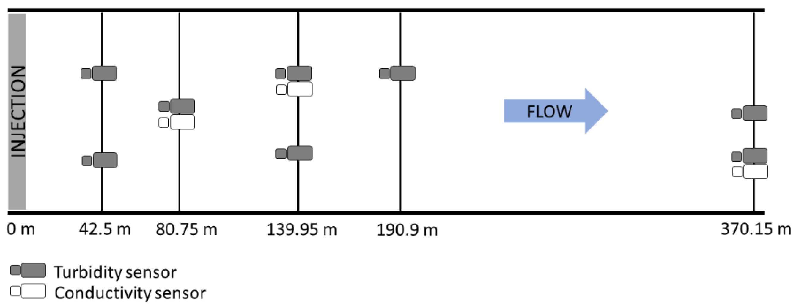
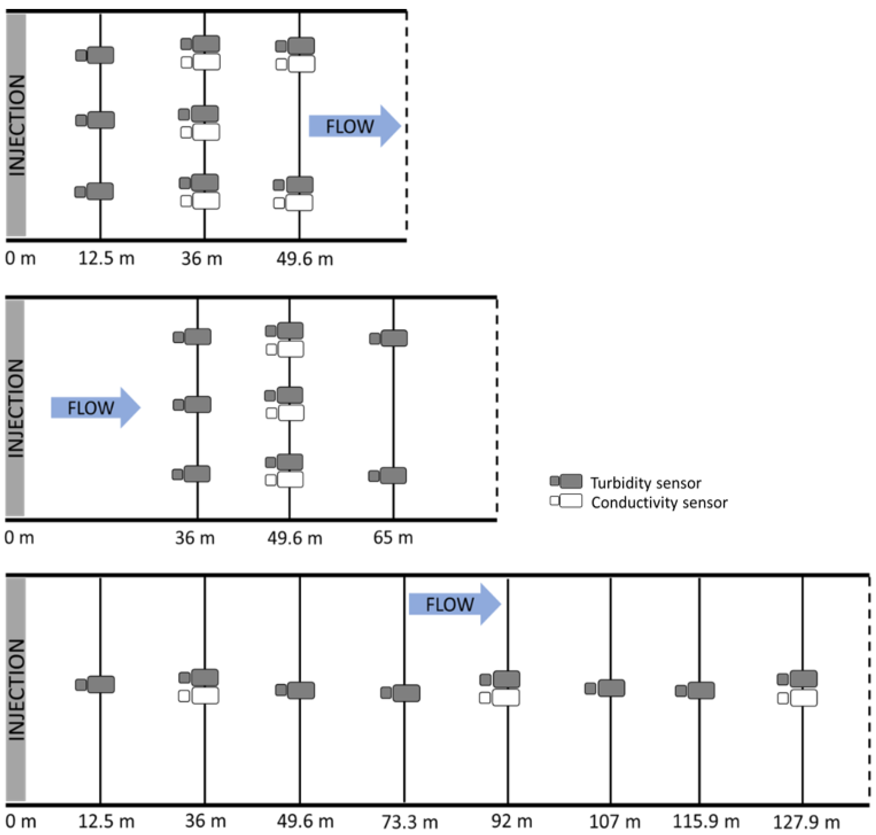
4.1. Field Experiments

Testing the accuracy and applicability of the 26 formulae involved a series of field experiments to collect empirical data on mixing processes in small channels followed by a suite of analytical procedures, including hydraulic modeling and curve fitting. Controlled tracer experiments with instantaneous mass injections of sodium chloride (NaCl) were conducted in two freshwater channels spanning a range of conditions: (i) a concrete-lined, trapezoidal channel that was geometrically and hydraulically simple (Figure 2); and (ii) a small, natural stream (Creighton Creek near Lumby, British Columbia), which was geometrically and hydraulically complex (Figure 3). Sodium chloride (NaCl) was used as an introduced foreign substance, with the expectation that there would be no transient storage and 100% mass recovery. NaCl solutions (approximately 100–200 g/L, well below saturation concentrations) were injected using a 2 m wide trough to ensure channel-wide distribution of the tracer and to facilitate complete lateral mixing within a short distance downstream. The trough was only slightly shorter than the width of the channels, conveniently avoiding any influence from the side walls at the injection locations. Vertical mixing was very rapid because the flow was shallow and turbulent, and density stratification was unlikely. The volume of water in the troughs was less than 3 litres and therefore had a negligible effect on the flow discharge. Salt concentration was measured indirectly using conductivity probes at a sampling frequency of 1 Hz over spans of 10–15 min.
Overall, 55 NaCl concentration curves were measured within the two channels: 25 in the concrete channel and 30 in the natural channel. The measurements were taken at several fixed locations downstream of the injection point, ranging anywhere from 80 m to 370.15 m for the concrete channel and from 12.5 m to 127.9 m for the natural channel. Over the course of the experiments, which also included turbidity monitoring (not discussed here), a variety of instrument deployment configurations were used (Figure 4 and Figure 5). At some locations, multiple sensors were deployed across the channel to verify that lateral mixing was uniform, which was the case at downstream locations far away from the injection site.
The concrete channel experiments were conducted on a single day, whereas the natural channel experiments were conducted over two subsequent days. Several different injections of salt and sediment were made throughout the course of the experiments, with sufficient time between injections to allow for complete flushing of the tracer out of the reach, as indicated by the return to background conditions. Hydraulic parameters for each channel were obtained from field measurements of channel geometry and flow discharge, complemented with HEC-RAS hydraulic modeling, from which cross-sectional averages of various parameters, such as mean flow velocity and mean flow depth, were obtained at different transects along the reach.

4.2. Analytical Procedures

HEC-RAS hydraulic models of the concrete channel and the natural channel were developed using multiple surveyed cross-sections along the study reach. After the model geometry was established, the flow conditions were calibrated to water surface elevations surveyed at each of the cross-sections for the discharge conditions encountered during the injection experiments. All hydraulic parameters used in subsequent calculations were reach-averaged values from the model simulations in order to avoid local influences due to varying cross-sectional geometry and roughness. The concrete channel had uniform geometry along its entire 370.15 m extent (Figure 2), whereas the natural channel had only a slight variation in width and depth (Figure 3), thereby justifying the use of reach-averaged values.
Reach-averaged values of the cross-sectional area and mean flow velocity from the HEC-RAS simulations were used in combination with the NaCl plume time series to estimate reach-averaged values for Kx. The Hayami analytical solution [7,24] to the one-dimensional ADE (Equation (2)) was used for this purpose:
C ¯ ( x , t ) = Mx 2 A U ¯ t π K x t exp ( ( x U ¯ t ) 2 4 K x t )
where M = tracer mass injected (M), A = cross-sectional area (L2), and other terms are as previously defined. The curve fitting process to the measured time series involved adjusting the longitudinal dispersion coefficient incrementally until perfect agreement (i.e., 0% deviation) was reached for the peak concentration between the measured and modelled plumes. The peak concentration fitting method was chosen rather than an overall best-fitting method (e.g., maximizing the coefficient of determination [R2] between observed and modeled curves) due to the long tails normally observed in plumes from real streams in comparison to the normal distribution shape predicted by Equation (2). Time to peak concentration and total plume duration were also evaluated as a means of checking the reliability of the solutions, and deviations between the modeled and measured plumes averaged around 4% and 30%, respectively (Table S2). However, there are no free parameters in Equation (2) to adjust these plume attributes once a value for Kx has been fixed to reproduce the peak concentration. Adjustments for tracer loss were made in a small number of instances when 100% recovery was not achieved downstream or to compensate for the uncertainty associated with the measured or estimated discharge.
Even though Kx values were calculated for all of the 55 measured plumes, only a small subset was used to test the empirical formulae. The reason is that the theory for one-dimensional advection-dispersion assumes that complete channel-wide mixing and equilibrium has been attained. In practice, this is difficult to achieve with slug injections of tracer in natural systems, and there is a distance downstream of the injection site where advection dominates over dispersion (referred to as the ‘convective’ or ‘advective’ zone) [5,25]. The predicted length of the advective zone and its implications for the longitudinal dispersion coefficient calculation are addressed in more detail in Appendix A, where we also discuss the uncertainty associated with field measurements of dispersion in small channels.
The accuracy of the predictive formulae for the longitudinal dispersion coefficient was assessed by calculating the relative percent error, as follows:
Relative   %   error = Predicted   value   observed   value Observed   value × 100
The relative percent error indicates whether the predicted values overestimate or underestimate the observed (true) values, which is a crucial concern when dealing with drinking water safety. It is important to highlight that this statistic is asymmetric in its range because a value of zero for the longitudinal dispersion coefficient is the minimum possible; therefore, the lower limit of the relative percent error is −100%, while the upper limit is + infinity.
To evaluate how well the predicted values of the longitudinal dispersion coefficient based on the 26 formulae performed in simulating the temporal evolution of the concentration curves, the predicted Kx values were used to model each of the NaCl injection experiments in turn. The modeled curves from the one-dimensional ADE solution were compared to the observed plume data acquired only in the equilibrium zone, and four attributes of the curves were selected to assess accuracy: start time of initial rise in concentration above background levels, peak concentration level, peak time (time from initial rise to peak concentration), and total duration of the plume. The accuracy of each modeled parameter was assessed according to the relative percent error (Equation (3)). The relative errors for individual runs were averaged across all runs for each of the two channels, and the level of agreement for each modeled parameter was classified according to the visual color scale shown in Figure 6. Finally, the overall level of agreement for each formula was defined according to the parameter that had the worst level of agreement.

5. Results

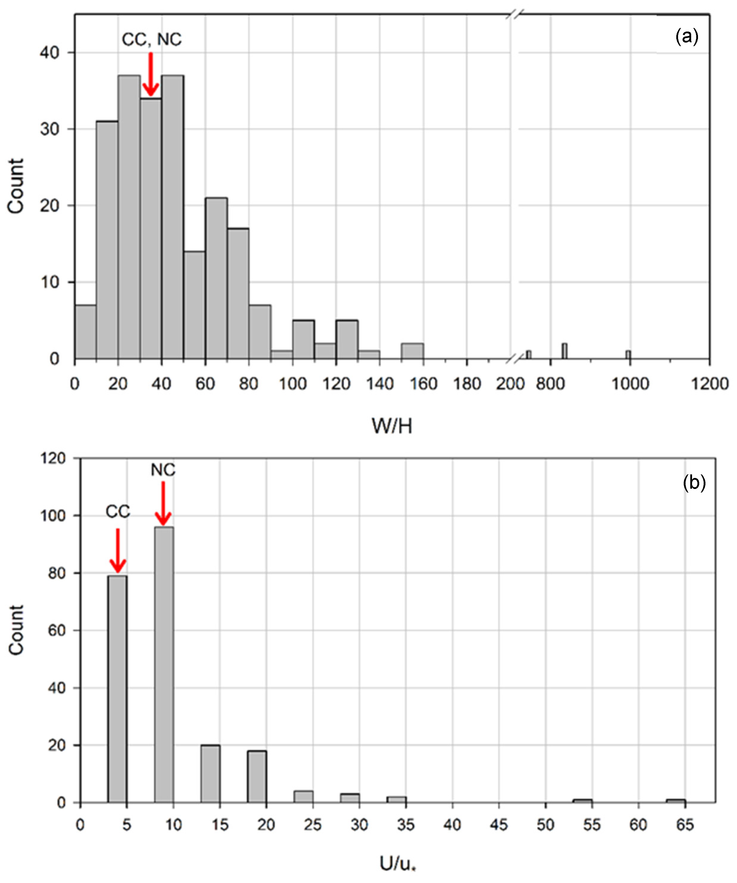
5.1. General Hydraulic Conditions

Table 1 shows the reach-averaged characteristics of the channels obtained from HEC-RAS simulations. These values conform well with actual measurements at a number of cross-sections of flow velocity and depth, which were constant along the 370 m length of the concrete channel and varied only slightly from cross-section to cross-section along the 130 m study reach of the natural channel. The advection velocities of the plume peaks were identical across all runs for each channel regardless of measurement location, indicating that discharge was steady and uniform during the experiments.

5.2. Quantification of Kx Values Based on Field Measurements

Based on the analysis presented on Appendix A, only the runs with measurements downstream of the advection zone were selected, reducing the number of viable cases to eight (of 25) plumes in the concrete channel and only two (of 30) plumes in the natural channel. All of the viable cases were from the most downstream measurement location; this demonstrates that significant downstream lengths are needed to obtain complete mixing. Indeed, a set of parallel experiments conducted in a 2 m wide, semi-natural drainage ditch yielded no viable measurements in the equilibrium zone, despite measurement locations as far as 90 m downstream of the injection point. Figure 7 shows several measured concentration curves alongside modeled concentration curves based on the calculated values of Kx, indicating that the fit is excellent (R2 = 0.91 for the concrete channel and R2 = 0.96 for the natural channel) at the downstream locations but not ideal for those locations deemed to be in the advective zone.
Table 2 shows the observed longitudinal dispersion coefficients and Peclet numbers for the most downstream measurement locations, deemed to be in the equilibrium zone. All other instrument positions farther upstream were not viable because they were estimated to be in the advective zone, where lateral mixing was predicted to be incomplete, despite using trough injection. These measurements in the advective zone produced longitudinal dispersion coefficients that were much smaller than those measured farther downstream (Appendix A). Confirmation of the (in)completeness of horizontal mixing, and hence the extent of the advection zone, came from instruments positioned across the channel at strategic transects (Figure 4 and Figure 5), which reaffirmed that the most downstream measurement locations were likely within the equilibrium zone.

5.3. Comparison of Kx Values from Formulae and from Field Measurements

Table 3 shows the reach-averaged hydraulic parameters from the HEC-RAS modelling for the sampling locations in the equilibrium zone, which are only slightly different from those reported in Table 1 for all runs and all locations. These hydraulic parameters were used to estimate the longitudinal dispersion coefficient from the 26 predictive formulae presented in Table S1, and the results are shown in Table 4.
There are order-of-magnitude differences among the models. For the concrete channel, the maximum value of the longitudinal dispersion coefficient was estimated by the formula from Oliveira et al. [21], Kx = 79.26 m2 s−1, whereas the smallest value was predicted by the formula of Elder [27], where Kx = 0.03 m2 s−1. For the natural channel, the maximum value was estimated by the formula from Koussis and Rodríguez-Mirasol [30], Kx = 6.84 m2 s−1, while the smallest value was predicted by the Ribeiro et al. [33] formula, where Kx = 0.01 m2 s−1. None of the formulae was able to yield accurate predictions of the longitudinal dispersion coefficient in both the concrete and natural channels, although some formulae performed well in one channel but not the other channel.

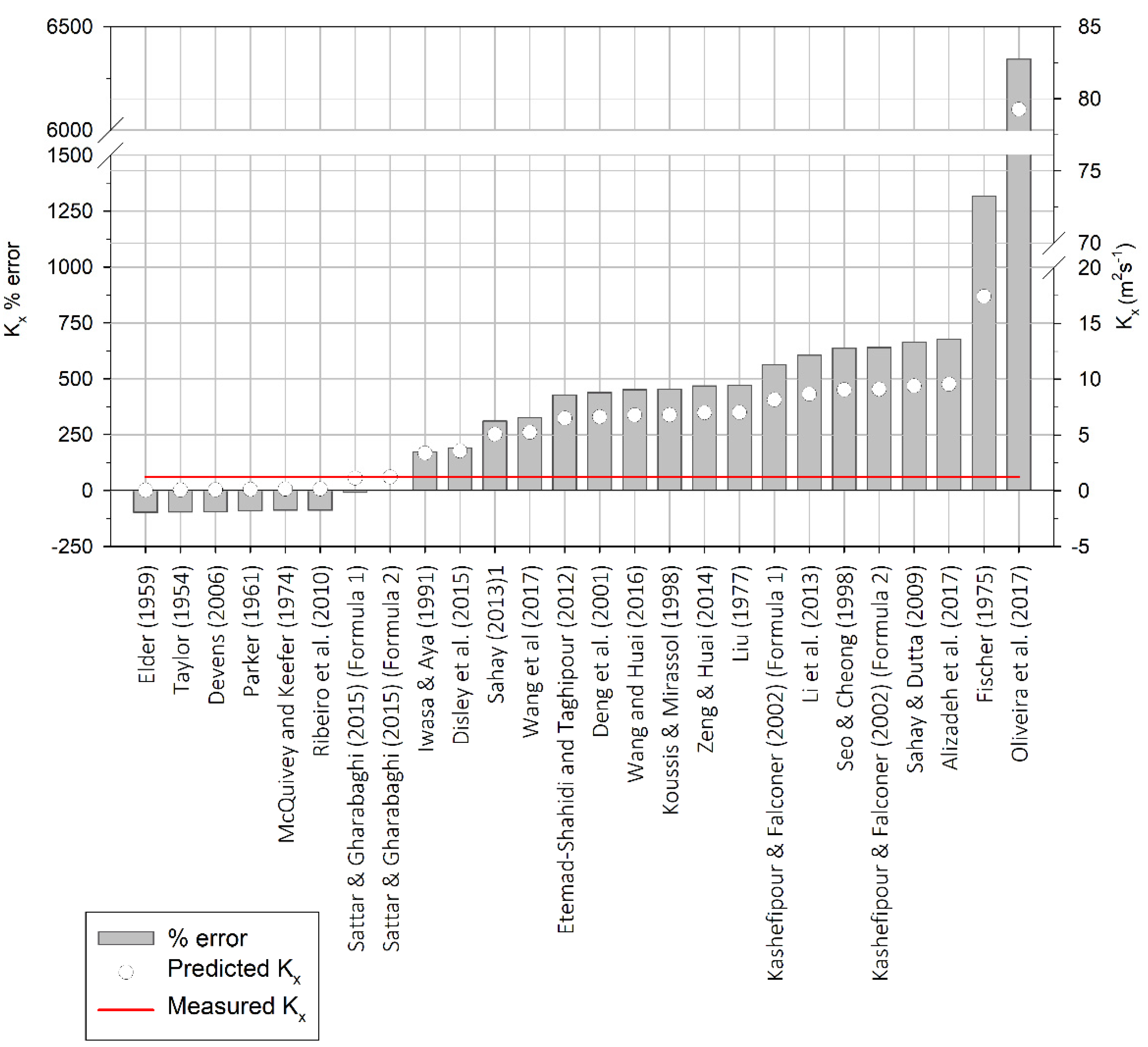
5.3.1. Concrete Channel Results

The majority (19 out of 26) of the formulae overestimated the value of the longitudinal dispersion coefficient in the concrete channel (Figure 8). The relative errors ranged from −100% (underestimation) to greater than 1000% (overestimation).
Relative errors between the modeled and observed curves were estimated for each of the curve attributes (i.e., peak concentration, time to peak, time to start, plume duration) and for each run. The averaged results for the concrete channel are presented in Table 5. The two formulae by Sattar and Gharabaghi [13] showed excellent agreement with the observed data. They predicted the peak concentration, peak time, start time, and duration of the curve with less than 10% absolute error. The formulae by Iwasa and Aya [23], Disley et al. [12], Sahay [35], and Wang et al. [17] provided fair agreement with the observed data. All the other formulae were classified as providing poor agreement with the observed data, mostly because of errors in the duration parameter.

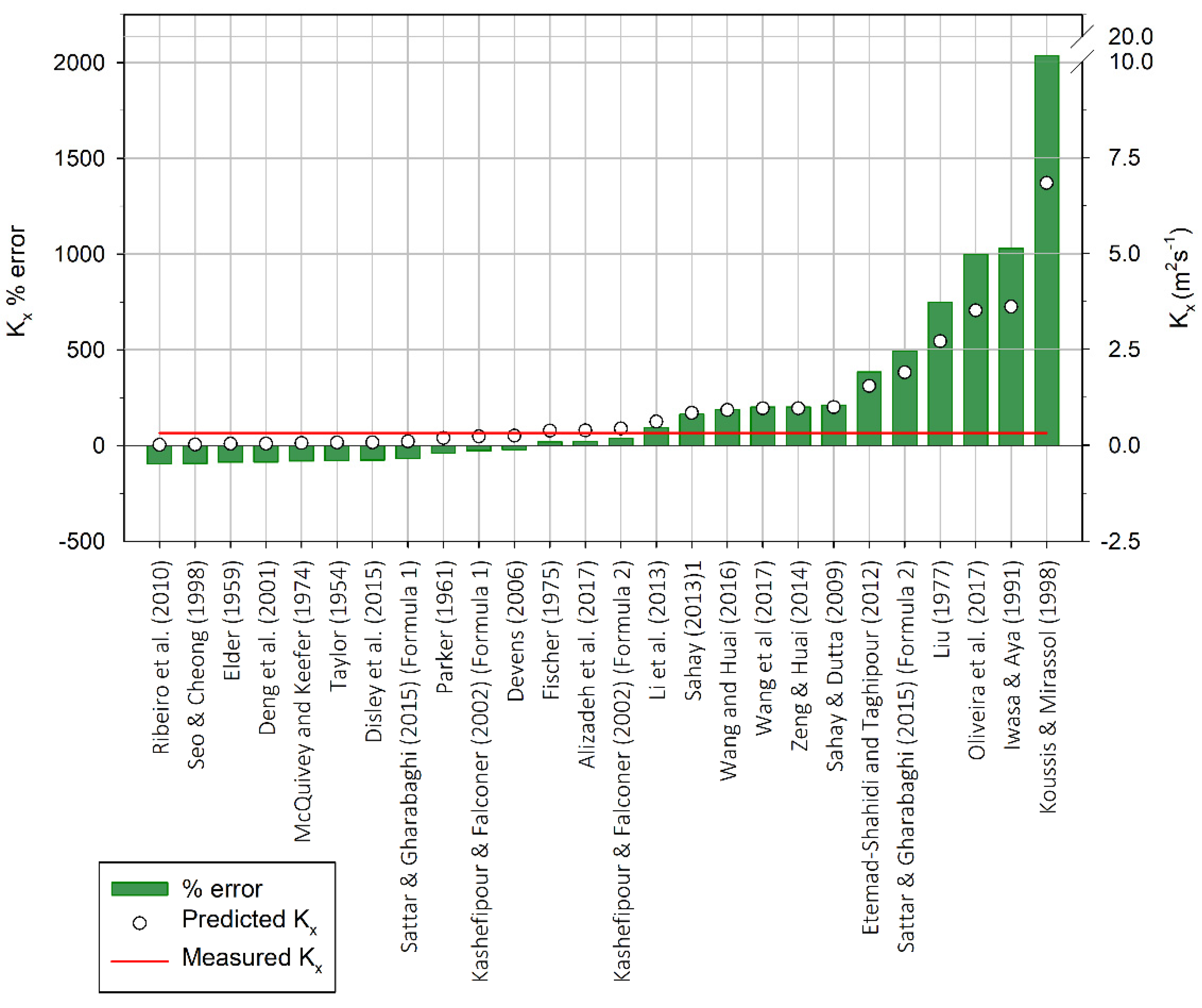
5.3.2. Natural Channel Results

Similar to the concrete channel, most formulae (15 out of 26) overestimated the value of the longitudinal dispersion coefficient in the natural channel (Figure 9). The relative errors ranged from −100% (underestimation) to greater than 1000% (overestimation).
The formulae by Devens [11] and Kashefipour and Falconer (F1) [32] had the best performance (excellent agreement), with all four parameters predicted within 25% absolute error (Table 6). The formulae from Parker [10], Fischer [28], Alizadeh et al. [16], Kashefipour and Falconer (F2) [32], Li et al. [34], Sahay [35], Wang and Huai [19], and Wang et al. [17] were classified as having good agreement with the observed data. All the remaining formulae (16) were classified as having fair or poor agreement with the observed data, including the two formulae by Sattar and Gharabaghi [13], which performed best in the concrete channel.

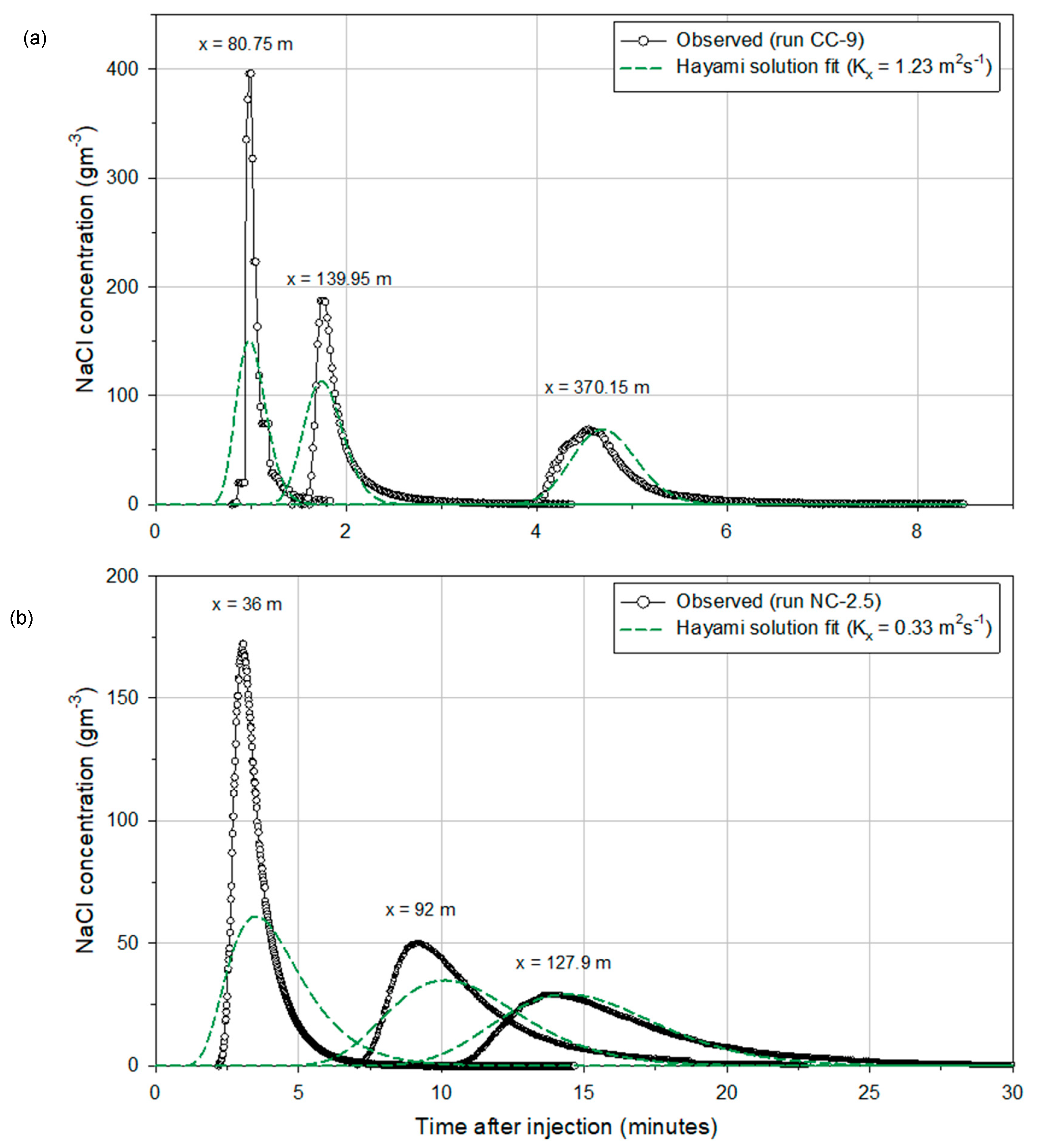
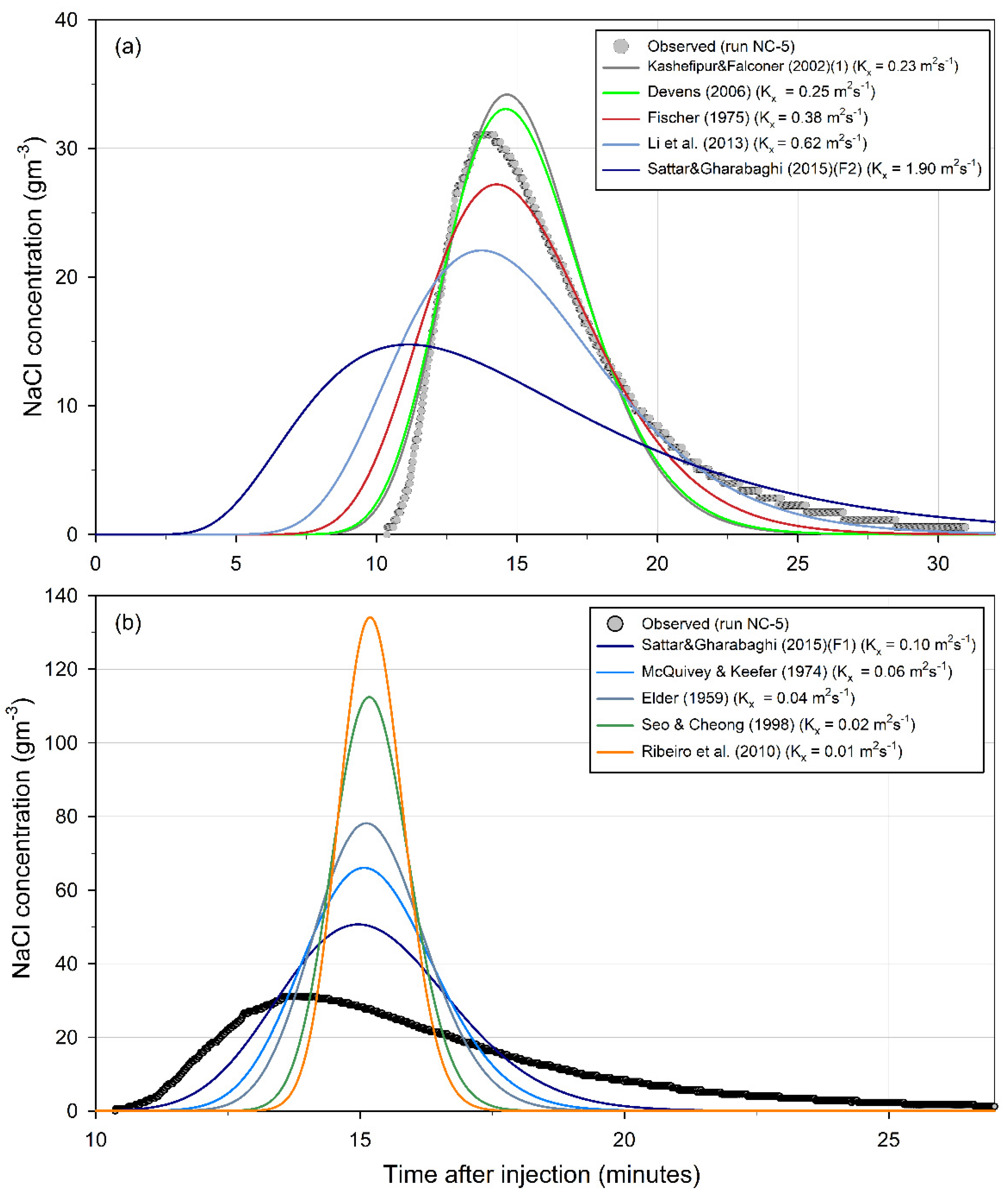
5.3.3. Comparison of Measured and Modeled Plumes

Figure 10 and Figure 11 show a series of simulated tracer curves (solid lines) for the concrete channel and natural channel, respectively, using a sample of formulae-derived Kx values that span the range from smallest to largest. Also shown on each of the panels is the measured concentration time series (open circles) that was collected for the hydraulic parameters and instrument locations used to create the simulated curves. The upper panels (Figure 10a and Figure 11a) show the simulated curve that most closely aligns with the measured curve based on a value of Kx produced by one of the 26 formulae as well as several other simulated curves with Kx values from other formulae that yield overestimates of the measured longitudinal dispersion coefficient. The lower panels (Figure 10b and Figure 11b) show simulated curves based on underestimates of Kx.
The modelled curves in Figure 10 and Figure 11 demonstrate that when the predicted Kx from a formula is greater than the observed Kx, the peak concentration is underestimated; conversely, when the predicted Kx is less than the observed Kx, the peak concentration is overestimated. In addition, the time to peak concentration advances ahead of the measured peak when the predicted Kx is greater than the measured Kx, and vice versa. The degree of deviation of the simulated curves from the measured curves increases as the predicted Kx deviates further from the measured Kx. Large values of Kx produce simulated curves that are flatter, broader, and asymmetric, whereas small values of Kx produce simulated curves that are peaked, short in duration, and almost symmetric.

6. Discussion

6.1. General Performance of Kx Formulae

A key finding of this study is that peak contaminant concentrations are generally poorly predicted when relying on most of the 26 formulae proposed in the literature to model mixing in small streams. Yet, peak concentration is of extreme importance for water quality management. In the case of turbidity plumes, mainly caused by suspended sediment events, if the concentration is above certain regulatory limits, a ‘boil water’ advisory alert is triggered, with adjustments required for drinking water treatment processes. The majority of the formulae yielded overestimations of the longitudinal dispersion coefficient and, hence, underestimations of the peak concentration, thereby potentially affecting health outcomes (i.e., failing to trigger alerts). Several studies in the literature have reached similar conclusions about the overestimation of Kx using a range of formulae (e.g., [1,11,36,37]). This is of relevance to regulatory compliance because it suggests that the probability of a modeler choosing, at random, a formula published in the literature that will underestimate the peak concentration is greater than selecting a formula that will predict a concentration that is equal to or greater than the expected concentration. Human health may be placed at risk because predicted concentrations of pollutants will be smaller than what is actually in the water during an event such as a hazardous waste spill.
The curve attribute that was predicted with the best accuracy was time to peak concentration, and it was consistently so for both channel types. For the concrete channel, 25 of 26 formulae yielded excellent agreement (within ±25%) between predicted and observed peak times, while in the natural channel, 22 of 26 provided excellent agreement. El Kadi Abderrezzak et al. [22] similarly noted small percentage errors (average of 5%) for the prediction of peak times using data from a laboratory flume. However, this is not a particularly stringent test for model performance because the peak time is governed mainly by the advection speed, which dictates how quickly the mass centroid is conveyed along the channel. The dispersion process, in contrast, affects the spread of the plume but not the conveyance of the mass centroid. The range of relative error for the peak time in the concrete channel (−35% to 4%) was smaller than the range of error in the natural channel (−83% to 18%), suggesting that the non-uniform character of natural channels increases the uncertainty around predicted plume travel times, likely because of flow unsteadiness through riffles and pools and around meander bends or because of transient storage effects.
For both channel types, the errors for the predicted interval between the time of injection to the initial rise in concentration (i.e., start time of the plume) were slightly greater than the errors for peak time. The reason for this is that the peak time is dependent mainly on the advection speed, whereas the start of the plume (as well as the total duration) is also dependent on dispersion at the leading edge of the plume (and tail of the plume for duration). The formulae that were able to predict the peak concentration with less than 25% absolute error all had the smallest error for the plume duration, but they also tended to underestimate the start times of the curves. The likely reason for this is that the one-dimensional ADE produces less skewed curves (i.e., more symmetric) than the observed curves. As the spread of the plume increases, the peak decreases; therefore, these two variables are closely related through mass conservation.
The total plume duration was associated with the largest errors among the four parameters considered. However, Rutherford [5] noted that the plume time series in real channels tends to display asymmetry, with long tails that are not well predicted by the one-dimensional ADE model. Part of the error in the duration parameter can be attributed to the inability of the one-dimensional model to provide accurate simulations of three-dimensional mixing. In other words, the lack of agreement between predicted and observed values is not solely linked to errors in the longitudinal dispersion coefficient but also to the basic model (Equation (1)) that was used in this study (and the majority of others) to analyze the measured curves and simulate the artificial curves. Arguably, the total duration of the plume is of lesser concern to water quality management than peak concentration, so the errors associated with plume duration may not be a significant regulatory concern. Nevertheless, cumulative impacts on aquatic organisms and ecosystems depend on both concentration and duration if plumes are long-lasting.

6.2. Comparative Performance of Kx Formulae

A simple comparison of the percent error in the values of the longitudinal dispersion coefficient (Table 7) demonstrates that: (1) eight of the formulae underestimated the longitudinal dispersion coefficient in both channels; (2) fourteen formulae overestimated the longitudinal dispersion coefficient in both channels; and (3) four formulae overestimated the coefficient in the concrete channel but underestimated it in the natural channel. No similarities were found between the formulae that overestimated the coefficient in the concrete channel but underestimated it in the natural channel, except that all four had a coefficient >1 for the U ¯ / u ratio and that their calibrating data sets included the data set from Seo and Cheong [31]. However, this was also true for other formulae, so it seems unlikely that there is a consistent bias that can be identified as regards the parameterization of the formulae.
None of the formulae was able to predict the dispersion process with excellent or good agreement in both channels. However, the two formulae from Sattar and Gharabaghi [13] had the smallest combined relative errors in peak concentration when considering both channel types, as shown in Figure 12, despite performing more poorly in the natural channel than the Devens [11] formula.
The formula from Devens [11] had excellent agreement for the natural channel but not the concrete channel. This result is unsurprising because the formula was calibrated using data solely from small channels that had similar characteristics to the natural channel in this study. The two formulae from Kashefipour and Falconer [32] also performed well for the natural channel, especially for predicting peak concentration. None of these formulae performed well in the concrete channel, likely because they were not calibrated to supercritical flow conditions. It is interesting to note that these three formulae have very different structural forms, and yet they all performed well on the natural channel, which is, perhaps, an indication of how important it is to calibrate the model against data that characterize the channel type of interest (i.e., small versus large).
A primary factor to consider when interpreting the results from this study is the substantial difference in relative roughness of the concrete channel versus the natural channel. The effects of surface roughness tend to be most important for channels that have large W/H ratios, in contrast to narrow, deep channels; however, the length scales of the frictional elements on the bottom boundary relative to the flow depth are also important. Relative roughness is parameterized indirectly in most of the formulae through the U ¯ / u ratio. Five of the seven formulae that had good agreement with observed data in the natural channel had an exponent on U ¯ / u larger than 1 [16,17,28,34,35], but none of these formulae had good agreement with the concrete channel, which could be due to the hydraulic smoothness of the concrete surface. Thus, it would appear that relative roughness is an important consideration for natural channels that have complex bed configurations, especially when flow depth is shallow, but perhaps not for channels that are hydraulically smooth, either because the beds are physically smooth or because flow is deep.
Another important consideration for this study is the fact that the flow in the natural channel was subcritical, whereas the flow in the concrete channel was supercritical. As far as we are aware, none of the 26 formulae were calibrated with data sets that included supercritical flows, but a few of the formulae [12,13] include the Froude number as a key parameter. Fischer et al. [38] suggested that flows with larger Froude numbers have lateral velocity distributions that are more uniform, which implies that lateral shear-induced dispersion is less important for mixing, and as a consequence, the longitudinal dispersion coefficient will be smaller. In general, the longitudinal dispersion coefficient should be inversely related to the Froude number, which explains the negative exponent in the Disley et al. [12] formula. The relationship is less clear in the Sattar and Gharabaghi [13] formulae, in which the Froude number is incorporated into several of the exponents. Once the Froude number is larger than 0.5 for Formula (1) (and the value 0.514Fr0.516 is larger than 0.5 + U ¯ u 0.42 U ¯ / u for Formula (2)), the exponent on W/H becomes negative. This means that with Fr < 1, W is more important than H, whereas with Fr > 1, H is more important than W. Therefore, the relative width is positively related to Kx in subcritical flows and negatively related to Kx in supercritical flows.

6.3. Contextual Considerations and Caveats

Overall, the error ranges reported in this research dealing explicitly with small channels are much larger than those reported in previous publications, which are often within ±100% (e.g., [1,22,32]). Some of the formulae performed better than others, and it is worth speculating on why this might be. In the case of formulae with empirical parameters, it seems reasonable to anticipate that they will perform best when applied to channels that are similar to those represented in the data set used to calibrate the formula, and more poorly when applied to dissimilar channels. A cursory analysis of the parameters utilized to derive each of the 26 formulae (Figure 1) pointed to the general absence of data on small channels in comparison to medium and large channels. The hydraulic characteristics of the channels used in this study (Table 1 and Table 3) were at the very small end of the data sets used by others, which leads to a more stringent test of many of the formulae. It is important to highlight that none of the calibration data sets used in previous studies included supercritical flow conditions (Fr > 1), despite the Froude number being incorporated into some of the formulae. In this study, the concrete channel experiments had values of Fr > 1.
Nevertheless, there are some similarities between the calibration data sets used in previous studies and the data used in this study, particularly with respect to the W/H and U ¯ / u ratios. Figure 13 shows that the W/H ratio for the study channels is in a modal position with respect to all other studies, whereas the U ¯ / u is very similar to all other studies despite being at the small end of the range, with large relative roughness. This suggests that relying on these two non-dimensional scaling parameters to predict the longitudinal dispersion coefficient for a specific channel may not produce accurate results without also considering the absolute size of the channel. In other words, a small channel may display different mixing dynamics than a large channel, even if these non-dimensional ratios suggest some degree of similarity.

7. Conclusions

Longitudinal dispersion coefficients from twenty-six formulae were compared to values obtained from field experiments on two small channels, and the relative performance of the formulae were evaluated based on the relative error. This is the most comprehensive test of these predictive formulae reported in the literature to date, and it included a cursory analysis of the calibrating data sets used by previous authors as well as a modeling exercise to simulate concentration curves and compare them to the field measurements. Given the general absence of small channels in the calibration data sets, it is unsurprising that most of the formulae were not capable of predicting the dispersion process in the two experimental channels in this study with better than ±50% accuracy. None of the formulae was capable of replicating the observed data trends in both the concrete channel and the natural channel with excellent or good agreement.
The majority of the formulae yielded overestimations of the longitudinal dispersion coefficient and, hence, underestimations of the peak concentration. This is of relevance in regulatory compliance because it suggests that the probability of a modeler choosing, at random, a formula from the literature that will underestimate the peak concentration is greater than choosing a formula that will predict the exact or larger concentrations.
The findings demonstrate that the predictive accuracy of the formulae is extremely variable, depending on the characteristics of the stream of interest (i.e., large versus small). It is challenging for any single formula to capture the large heterogeneity in dispersive mixing processes in natural channels using a single predictor variable such as relative width or relative roughness. Thus, many recent models incorporate several variables with complex functions in an attempt to span a range of stream conditions. However, the general absence of calibration data on small channels remains problematic. In the context of water quality assessments in small streams, it is advisable to use a formula that was calibrated with data from streams with similar characteristics to the channel of interest. This approach increases the likelihood of more accurate results, as was demonstrated in this study for the case of the natural channel and the better performance of the formulae proposed by Devens [11]. The two formulae from Sattar and Gharabaghi [13] had the best overall performance, being able to predict the concentrations with the best accuracy for both channel types. The results from this research indicate that it might be beneficial to develop formulae for the longitudinal dispersion coefficients that are more case-specific and can assure high levels of accuracy in a specific type of channel, instead of the more traditional approach of developing universally-applicable formulae with large degrees of uncertainty. The question of whether one-dimensional theory is applicable to small streams and creeks, given that many of the basic assumptions and limiting conditions are weakly violated, is a larger issue requiring further study.

Supplementary Materials

The following supporting information can be downloaded at: https://www.mdpi.com/article/10.3390/geosciences12070281/s1, Table S1: Empirical equations used to predict the longitudinal dispersion coefficient, Table S2: Relative error between the modeled (best-fit Kx) and observed sodium chloride concentration curves in the concrete and natural channels (equilibrium zone).

Author Contributions

Conceptualization, M.A.N. and B.O.B.; Formal analysis, M.A.N.; Funding acquisition, B.O.B.; Methodology, M.A.N. and B.O.B.; Supervision, B.O.B.; Writing—original draft, M.A.N.; Writing—review and editing, B.O.B. All authors have read and agreed to the published version of the manuscript.

Funding

This research was supported by the BC Ministry of Forests, Lands, Natural Resource Operations and Rural Development [contract #RA19DOS026] and by the Okanagan Basin Water Board [WCQI Grant].

Data Availability Statement

The data supporting the analysis are available from the senior author upon request.

Acknowledgments

We thank Deborah Roberts and Jeff Curtis, for their valuable insights during the development of this research. We are very grateful for the field assistance provided by Alexander MacDuff, Taylor McRae, Martin Guttridge, Lisa Hettrich, Polina Orlov, Sierra Collins, and Jeff Curtis. Many thanks to Christian St. Pierre from the BC Ministry of Forests, Lands, Natural Resource Operations and Rural Development (FLNRORD), who participated in the field experiments and conducted some of the discharge measurements.

Conflicts of Interest

The authors declare no conflict of interest. The funders had no role in the design of the study; in the collection, analyses, or interpretation of data; in the writing of the manuscript, or in the decision to publish the results.

Appendix A. Advective Zone Length Calculations and Their Inherent Uncertainties

An issue that looms large in the background of all studies dealing with one-dimensional advection-dispersion in rivers or streams is the uncertainty of knowing whether the measurements were taken in the advective zone, where the basic 1D theory does not apply, or in the equilibrium zone, where Fickian constructs are believed to be reasonably applicable. Strictly speaking, plume measurements in the advective zone should not be used to test longitudinal dispersion coefficient formulae [5,25]. Values of Kx in the advective zone are expected to change non-linearly with downstream distance, along with other attributes of the concentration distribution (e.g., variance, skewness). In the equilibrium zone, Kx should be constant, while variance should increase linearly, as required by Fickian theory [5,7]. Equilibrium mixing conditions are anticipated to occur at a downstream location far away from the injection point, where shear action and turbulent diffusion reach equilibrium, i.e., the tracer particles have experienced the entire extent of the vertical and lateral velocity fields and are uniformly distributed over the cross-sectional area of the channel [5]. However, there remains considerable ambiguity in the literature about how to parameterize this critical distance (i.e., the length of the advective zone).
A number of approaches have been proposed to predict the downstream distance from the point of injection needed to achieve complete mixing. Fischer [38], for example, proposed a Lagrangian time scale for equilibrium mixing, from which can be derived the following theoretical expression for the length of the advective zone [25]:
L A = α U ¯ L t 2 ε y = α U ¯ L t 2 β Hu
where LA = advective zone length (L), U ¯ = average flow velocity (LT−1), Lt = transverse length scale (L), εy = depth-averaged lateral dispersion coefficient (L2T−1), H = flow depth, u = shear velocity (LT−1), and α , β are coefficients that depend on the type of source (point or line), the location of injection (mid-channel or near the banks), channel roughness, presence of dead zones, and sinuosity, among others [5,7,25,39,40]. The transverse length scale is the distance between the thread of maximum velocity and the farthest bank, and by convention, it is taken as Lt = 0.5 W in symmetrical channels and Lt = 0.7 W in natural channels [38], where W = channel width. Values of reach-averaged shear velocity were obtained based on the HEC-RAS hydraulic model results.
Estimates of the advective zone length (LA) for this study were calculated on the basis of Equation (A1) using the broad range of empirical coefficients commonly reported in the literature. As reported by Rutherford [5] and Shucksmith et al. [25], the value of α varies from 0.2 [41]), to 0.5 [42], to 1 [43]. The value β was estimated to be 0.6 for natural streams [35,44], although 0.15 was suggested for a straight, rectangular flume [32]. Substituting representative values of α / β in Equation (A1), the estimates of advective zone length, LA, ranged from 101 m to 507 m for the concrete channel and 41 m to 204 m for the natural channel, as shown graphically in Figure A1. This suggests that the most downstream measurement locations in this study were either within the equilibrium zone or at least close to the transition from advective to equilibrium conditions. In an extensive study of available data on dispersion in large rivers, Nordin and Sabol ([7], p. 54) concluded that
“…there is no convincing evidence in the empirical data that the mixing length of Equation (20) [i.e., Equation (A1) in this paper with α / β = 1.8 as recommended by Fisher [45]] or the time scale of Equation (36) is a sufficient criterion to classify the dispersion process…Actually, the mixing length criterion is somewhat arbitrary, and there are possibilities for wide deviations from Equation (20).”
Figure A1. Advective zone length estimates based on the α / β coefficient range and location of farthest downstream measurements in the concrete (grey) and natural (green) channels.
Geosciences 12 00281 g0a1
In practice, if sufficient data were available (which is rarely the case), the start of the equilibrium zone could be identified as the downstream location where the spatial variance of the concentration curves begins to increase linearly with time [5,7,25]. Plots of variance and skewness based on our measured plumes were inconclusive in this regard because there were too few measurement locations in the downstream direction to discern trends with any degree of confidence. Moreover, concentration time series observed in real channels, including ours, often have long tails that affect the rate of increase of the variance [7], thereby confounding a graphical approach to determining the distance to the equilibrium zone.
In this study, the Peclet Number (Pe) was calculated as a potential indicator of the degree to which the measurements taken in the downstream direction were likely to have been made in the advective zone or the equilibrium zone. The Peclet Number is a dimensionless number that defines the relative importance of advective and dispersive fluxes, defined as follows [36,45,46,47]:
Pe = U ¯ L K x
where L = characteristic length (L), and the other terms are as defined previously. In the one-dimensional case considered here, the characteristic length (L) is the width of the channel (W), and the reach-averaged velocity was used for U ¯ . The values of Kx were based on the curve-fitting procedures described above (i.e., identical peak concentration in measured and modelled plumes), thereby yielding a unique estimate of Kx for every measurement location for every injection run. In general, flow is considered to be advection-dominated if Pe ≳ 5 and dispersion-dominated if Pe ≲ 1 [48]. Although the Peclet Number is not a direct indicator of whether equilibrium mixing has been achieved, it does provide a means of assessing whether flow conditions are likely to be dominated by dispersive processes that are central to equilibrium mixing. As shown in Figure A2, the Peclet Number decreased rapidly from Pe > 10 near the injection line to values of Pe ≲ 3 at the farthest downstream measurement point in both channels. The trajectory of the trend curve flattens with downstream distance, which indicates that Kx is declining asymptotically to a stable value, as required by the Fickian theory for equilibrium mixing. This suggests that the measurements taken at the most downstream locations were likely within the equilibrium zone. Accordingly, for this study, only concentration curves measured at the farthest downstream locations for both channels were used for testing of the 26 formulae, which reduced significantly the number of viable plumes used in the testing process (from 55 to 10), as noted in Section 5.2.
Figure A2. Downstream trends in Peclet Number in the concrete (grey) and natural (green) channels. The solid dots are the mean values for each measurement location, and the whiskers show ± 1 standard deviation.
Geosciences 12 00281 g0a2
In dispersion experiments on natural systems, there will always be some degree of uncertainty as to whether measurement locations are positioned far enough downstream to be considered in the equilibrium zone or at the transitional margin from the advective zone to the equilibrium zone. Nevertheless, the use of a lateral injection trough in our experiments ensured that channel-wide mixing was facilitated a short distance downstream of the injection site. This was verified by multiple sensors located in the spanwise direction at select cross-sections (Figure 4 and Figure 5). In addition, the use of the Peclet Number provides some confidence that the downstream measurements were far enough away from the injection point to enable complete mixing by dispersion. Nordin and Sabol ([7], pg. 54) noted that
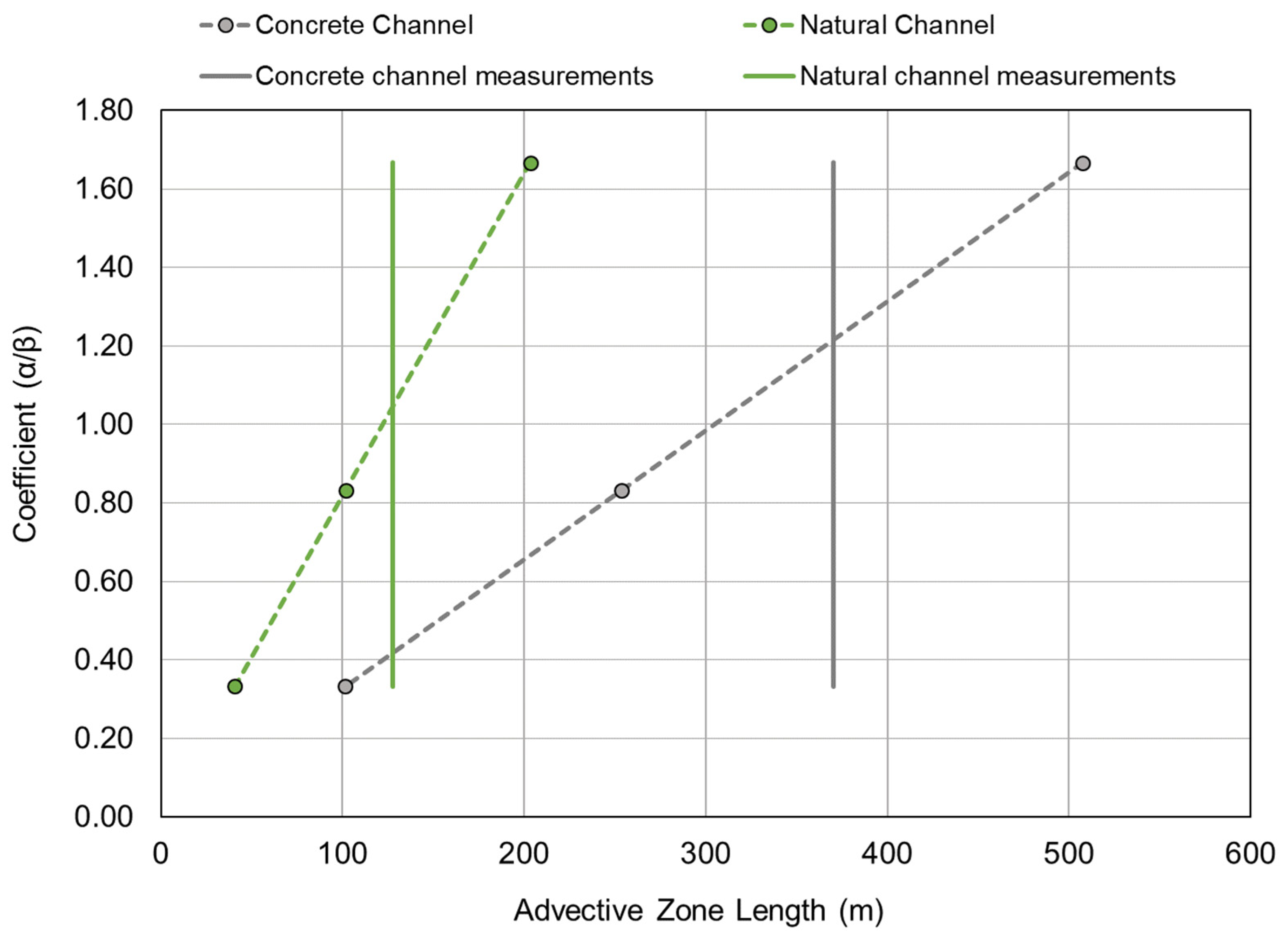
“from a practical point of view, if the convective influence extends downstream much farther than the length given by Equation (20) (Equation (A1) in this paper with α / β = 1.8), the one-dimensional model is not likely to be of much value because the dispersant would be completely out of the reach of interest before the theory applies.”
This is likely the reality for most small streams and creeks where channel characteristics can change rapidly over short distances, thereby leading to non-uniform flow conditions that pose serious challenges to a simple 1D model of dispersive processes.

References

  1. Camacho Suarez, V.V.; Schellart, A.N.A.; Brevis, W.; Shucksmith, J.D. Quantifying the impact of uncertainty within the longitudinal dispersion coefficient on concentration dynamics and regulatory compliance in rivers. Water Resour. Res. 2019, 55, 4393–4409. [Google Scholar] [CrossRef]
  2. Launay, M.; Le Coz, J.; Camenen, B.; Walter, C.; Angot, H.; Dramais, G.; Faure, J.B.; Coquery, M. Calibrating pollutant dispersion in 1-D hydraulic models of river networks. J. Hydro-Environ. Res. 2015, 9, 120–132. [Google Scholar] [CrossRef] [Green Version]
  3. Holley, E.R.; Siemons, J.; Abraham, G. Some aspects of analyzing transverse diffusion in rivers. J. Hydraul. Res. 1972, 10, 27–57. [Google Scholar] [CrossRef]
  4. Julien, P.Y. Erosion and Sedimentation, 2nd ed.; Cambridge University Press: Cambridge, UK, 2010; pp. 1–371. [Google Scholar] [CrossRef]
  5. Rutherford, V.J.C. River Mixing; John Wiley & Sons, Ltd.: New York, NY, USA, 1994; pp. 1–347. [Google Scholar] [CrossRef]
  6. Fick, A. On liquid diffusion. J. Membr. Sci. 1995, 100, 33–38. [Google Scholar] [CrossRef]
  7. Nordin, C.F.; Sabol, G.V. Empirical data on longitudinal dispersion in rivers. In US Geological Survey Water-Resources Investigations Report; U.S. Geological Survey: New York, NY, USA, 1974; Volume 74-20, 332p. [Google Scholar] [CrossRef]
  8. Van Genuchten, M.T.; Leij, F.J.; Skaggs, T.H.; Toride, N.; Bradford, S.A.; Pontedeiro, E.M. Exact analytical solutions for contaminant transport in rivers 1. The equilibrium advection-dispersion equation. J. Hydrol. Hydromech. 2013, 61, 146–160. [Google Scholar] [CrossRef]
  9. McQuivey, R.S.; Keefer, T.N. Simple method for predicting dispersion in streams. J. Environ. Eng. Div. 1974, 100, 977–1011. [Google Scholar] [CrossRef]
  10. Parker, F.L. Eddy diffusion in reservoirs and pipelines. J. Hydraul. Div. 1961, 87, 151–171. [Google Scholar] [CrossRef]
  11. Devens, J.A. Quantification of Longitudinal Dispersion Coefficient in Streams with the Use of Neutral Tracer. Master’s Thesis, Federal University of Ouro Preto, Ouro Preto, Brazil, 2006. Available online: http://www.repositorio.ufop.br/jspui/handle/123456789/2226 (accessed on 18 July 2022).
  12. Disley, T.; Gharabaghi, B.; Mahboubi, A.A.; Mcbean, E.A. Predictive equation for longitudinal dispersion coefficient. Hydrol. Process 2015, 29, 161–172. [Google Scholar] [CrossRef]
  13. Sattar, A.M.A.; Gharabaghi, B. Gene expression models for prediction of longitudinal dispersion coefficient in streams. J. Hydrol. 2015, 524, 587–596. [Google Scholar] [CrossRef]
  14. Sahay, R.R.; Dutta, S. Prediction of longitudinal dispersion coefficients in natural rivers using genetic algorithm. Hydrol. Res. 2009, 40, 544–552. [Google Scholar] [CrossRef]
  15. Etemad-Shahidi, A.; Taghipour, M. Predicting longitudinal dispersion coefficient in natural streams using M5′ model tree. J. Hydraul. Eng. 2012, 138, 542–554. [Google Scholar] [CrossRef]
  16. Alizadeh, M.J.; Ahmadyar, D.; Afghantoloee, A. Improvement on the existing equations for predicting longitudinal dispersion coefficient. Water Resour. Manag. 2017, 31, 1777–1794. [Google Scholar] [CrossRef]
  17. Wang, Y.F.; Huai, W.X.; Wang, W.J. Physically sound formula for longitudinal dispersion coefficients of natural rivers. J. Hydrol. 2017, 544, 511–523. [Google Scholar] [CrossRef]
  18. Deng, Z.-Q.; Singh, V.P.; Bengtsson, L. Longitudinal dispersion coefficients in straight rivers. J. Hydraul. Eng. 2001, 127, 919–927. [Google Scholar] [CrossRef]
  19. Wang, Y.; Huai, W. Estimating the longitudinal dispersion coefficient in straight natural rivers. J. Hydraul. Eng. 2016, 142. [Google Scholar] [CrossRef]
  20. Zeng, Y.H.; Huai, W.X. Estimation of longitudinal dispersion coefficient in rivers. J. Hydro-Environ. Res. 2014, 8, 2–8. [Google Scholar] [CrossRef]
  21. Oliveira, V.V.; Mateus, M.V.; Gonçalves, J.C.D.S.I.; Utsumi, A.G.; Giorgetti, M.F. Prediction of the longitudinal dispersion coefficient for small watercourses. Acta Sci. Technol. 2017, 39, 291–299. [Google Scholar] [CrossRef] [Green Version]
  22. El Kadi Abderrezzak, K.; Ata, R.; Zaoui, F. One-dimensional numerical modelling of solute transport in streams: The role of longitudinal dispersion coefficient. J. Hydrol. 2015, 527, 978–989. [Google Scholar] [CrossRef]
  23. Iwasa, Y.; Aya, S. Predicting Longitudinal Dispersion Coefficient in Open-Channel Flows. In Proceedings of the International Symposium on Environmental Hydraulics, Hong Kong, China, 16–18 December 1991; pp. 505–510. [Google Scholar]
  24. Hayami, H. On the of Propagation of Flood Waves, Disaster Prevention Research Institute, Bulletin No. 1; Kyoto University: Kyoto, Japan, 1951; Available online: http://hdl.handle.net/2433/123641 (accessed on 18 July 2022).
  25. Shucksmith, J.; Boxall, J.; Guymer, I. Importance of advective zone in longitudinal mixing experiments. Acta Geophys. 2007, 55, 95–103. [Google Scholar] [CrossRef]
  26. Taylor, G. The dispersion of matter in turbulent flow through a pipe. Proc. R. Soc. A Math. Phys. Eng. Sci. 1954, 223, 446–468. [Google Scholar] [CrossRef]
  27. Elder, J.W. The dispersion of marked fluid in turbulent shear flow. J. Fluid Mech. 1959, 5, 544–560. [Google Scholar] [CrossRef]
  28. Fischer, H.B. Discussion of “Simple method for predicting dispersion in streams”. J. Environ. Eng. Div. 1975, 101, 453–455. [Google Scholar] [CrossRef]
  29. Liu, H. Predicting dispersion coefficients of streams. J. Environ. Eng. Div. 1977, 103, 56–69. [Google Scholar] [CrossRef]
  30. Koussis, A.D.; Rodríguez-Mirasol, J. Hydraulic estimation of dispersion coefficient for streams. J. Hydraul. Eng. 1998, 124, 317–320. [Google Scholar] [CrossRef]
  31. Seo, W.; Cheong, T.S. Predicting longitudinal dispersion coefficient in natural streams. J. Hydraul. Eng. 1998, 124, 25–32. [Google Scholar] [CrossRef]
  32. Kashefipour, S.M.; Falconer, R.A. Longitudinal dispersion coefficients in natural streams. Water Res. 2002, 36, 1596–1608. [Google Scholar] [CrossRef]
  33. Ribeiro, C.B.M.; da Silva, D.D.; Soares, J.H.P.; Guedes, H.A.S. Development and validation of an equation to estimate longitudinal dispersion coefficient in medium-sized rivers. Eng. Sanit. E Ambient. 2010, 15, 393–400. [Google Scholar] [CrossRef] [Green Version]
  34. Li, X.; Liu, H.; Yin, M. Differential evolution for prediction of longitudinal dispersion coefficients in natural streams. Water Resour. Manag. 2013, 27, 5245–5260. [Google Scholar] [CrossRef]
  35. Sahay, R.R. Predicting longitudinal dispersion coefficients in sinuous rivers by genetic algorithm. J. Hydrol. Hydromech. 2013, 61, 214–221. [Google Scholar] [CrossRef] [Green Version]
  36. Carr, M.L. An Efficient Method for Measuring the Dispersion Coefficient in Rivers. Ph.D. Thesis, University of Illinois, Urbana, IL, USA, 2007. [Google Scholar]
  37. Ahsan, N. Estimating the coefficient of dispersion for a natural stream. World Acad. Sci. Eng. Technol. 2008, 44, 131–135. [Google Scholar]
  38. Fischer, H.B.; List, E.J.; Koh, R.C.Y.; Imberger, J.; Brooks, N.H. Mixing in Inland and Coastal Waters; Academic Press, INC.: New York, NY, USA, 1979; p. 4. [Google Scholar]
  39. Fischer, H.B. The mechanics of dispersion in natural streams. J. Hydraul. Div. 1967, 93, 187–216. [Google Scholar] [CrossRef]
  40. Sharma, H.; Ahmad, Z. Transverse mixing of pollutants in streams: A review. Can. J. Civ. Eng. 2014, 41, 472–482. [Google Scholar] [CrossRef]
  41. Fischer, H.B. Longitudinal dispersion and turbulent mixing in open channel flow. Ann. Rev. Fluid Mech. 1973, 5, 59–78. [Google Scholar] [CrossRef]
  42. Sayre, W.W. Dispersion of Mass in Open Channel Flow. Ph.D. Thesis, Colorado State University, Fort Collins, CO, USA, 1968. [Google Scholar]
  43. Chatwin, P.C. The cumulants of the distribution of concentration of a solute in a solvent flowing along a straight tube. J. Fluid Mech. 1972, 51, 63–67. [Google Scholar] [CrossRef]
  44. Pannone, M. An analytical model of Fickian and non-Fickian dispersion in evolving-scale log-conductivity distributions. Water 2017, 9, 751. [Google Scholar] [CrossRef] [Green Version]
  45. Fischer, H.B. Dispersion predictions in natural streams. J. Sanit. Eng. Div. 1968, 94, 927–944. [Google Scholar] [CrossRef]
  46. Pannone, M.; Mirauda, D.; De Vincenzo, A.; Molino, B. Longitudinal Dispersion in Straight Open Channels: Anomalous Breakthrough Curves and First-Order Analytical Solution for the Depth-Averaged Concentration. Water 2018, 10, 478. [Google Scholar] [CrossRef] [Green Version]
  47. Aquino, T.; Aubeneau, A.; Bolster, D. Peak and tail scaling of breakthrough curves in hydrologic tracer tests. Adv. Water Resour. 2015, 78, 1–8. [Google Scholar] [CrossRef]
  48. Koussis, A.D.; Saenz, M.A.; Tollis, I.G. Pollution routing in streams. J. Hydraul. Eng. 1983, 109, 1636–1651. [Google Scholar] [CrossRef]
Figure 1. Frequency distribution of channel width in the data utilized to derive the predictive formulae of the longitudinal dispersion coefficient (Table S1).
Geosciences 12 00281 g001
Figure 2. Conductivity sensors in the middle section of the concrete channel, looking upstream toward the injection site in the far distance.
Geosciences 12 00281 g002
Figure 3. Conductivity sensors in the natural channel, looking upstream.
Geosciences 12 00281 g003
Figure 4. Instrument deployment configurations used in multiple experiments in the concrete channel.
Geosciences 12 00281 g004
Figure 5. Instrument deployment configurations used in multiple experiments in the natural channel.
Geosciences 12 00281 g005
Figure 6. Level of agreement between modeled and observed parameters based on the relative percent error.
Geosciences 12 00281 g006
Figure 7. Modeled concentration curves based on the equilibrium longitudinal dispersion coefficient versus measured concentration curves. (a) Concrete channel; sampling locations x = 80.75 m and x = 139.95 m were located in the advective zone, and x = 370.15 m was located in the equilibrium zone. (b) Natural stream; sampling locations x = 36 m and x = 92 m were located in the advective zone, and x = 127.9 m was located in the equilibrium zone.
Geosciences 12 00281 g007
Figure 8. Percent error of the longitudinal dispersion coefficient value obtained with the predictive formulas when compared with the best-fit average value from the Hayami solution for the concrete channel (red line).
Geosciences 12 00281 g008
Figure 9. Percent error of the longitudinal dispersion coefficient value obtained with the predictive formulas when compared with the best-fit average value from the Hayami solution for the natural channel (red line).
Geosciences 12 00281 g009
Figure 10. Modeled concentration curves utilizing the longitudinal dispersion coefficients obtained from a sample of predictive formulae in the concrete channel, 370.15 m downstream of the injection. Curve with round symbols shows the observed plume, which is a common reference for both graphs (note the scale change on both axes). (a) Formulae that underestimated the peak concentration. (b) Formulae that overestimated the peak concentration.
Geosciences 12 00281 g010
Figure 11. Modeled concentration curves utilizing the longitudinal dispersion coefficients obtained from a sample of predictive formulae in the natural channel, 127.9 m downstream of the injection location. Curve with round symbols shows the observed plume, which is a common reference for both graphs (note the scale change on both axes). (a) Formulae that underestimated the peak concentration. (b) Formulae that overestimated the peak concentration.
Geosciences 12 00281 g011
Figure 12. Peak concentration relative error for the concrete and natural channels.
Geosciences 12 00281 g012
Figure 13. Frequency distribution of the data utilized to calibrate the empirical formulas for the longitudinal dispersion coefficient in Table 1. (a) W/H frequency distribution; (b) U/ u frequency distribution. The red arrows indicate the ranges corresponding to channels in this study.
Geosciences 12 00281 g013
Table 1. Reach-averaged hydraulic characteristics of the study channels.
ChannelVelocity (m s−1)Flow Depth (m)Top Width (m)Shear
Velocity (m s−1)
Froude Number
Concrete1.290.052.240.111.86
Natural
(runs NC 1.1–1.3)
0.180.114.900.090.17
Natural
(runs NC 2.1–2.6)
0.150.083.710.080.17
Table 2. Observed longitudinal dispersion coefficients and Peclet numbers for the concentration curves located in the equilibrium zone.
Concrete Channel (Measurement Mocation 370.15 m)
RunKx (m2 s−1)Peclet NumberR2
CC-11.002.950.89
CC-2---
CC-31.122.630.79
CC-41.102.610.71
CC-51.302.220.84
CC-61.152.590.87
CC-71.651.770.95
CC-81.202.460.92
CC-91.232.400.91
AVG1.232.45
SD0.200.35
CV16%14
Natural Channel (Measurement Location 127.9 m)
RunKx (m2 s−1)Peclet NumberR2
NC-50.331.500.96
NC-60.311.600.86
AVG is the average; SD is the standard deviation; CV is the coefficient of variation; R2 is the coefficient of determination.
Table 3. Reach-averaged hydraulic characteristics for locations in the equilibrium zone of the two experimental channels.
VariableConcrete ChannelNatural Channel
Location (m)370.15127.9
W (m)2.273.58
H (m)0.050.09
U ¯ (m s−1)1.300.14
A (m2)0.110.31
Q (m3 s−1)0.1430.042
u (m s−1)0.110.08
W/H4539.78
U ¯ / u 121.75
S0.0250.012
Fr1.870.16
Si1.001.54
W = top width, H = flow depth, U ¯ = cross-sectional average flow velocity, A = flow area (m2), Q = discharge (m3s−1), u = shear velocity, W/H = aspect ratio, U ¯ / u = surface roughness ratio, S = frictional slope, Fr = Froude number, Si = sinuosity factor.
Table 4. Longitudinal dispersion coefficients for the concrete channel and natural stream estimated from the 26 predictive formulae (presented here in chronological order) in comparison to the observed value (top line, italics). The largest and smallest values are underlined and in bold type.
ReferenceConcrete ChannelNatural Stream
Kx (m2 s−1)Kx (m2 s−1)
Observed value (Hayami solution best-fit)1.230.32
Taylor (1954) [26]0.060.07
Elder (1959) [27]0.030.04
Parker (1961) [10]0.110.19
McQuivey and Keefer (1974) [9]0.150.06
Fischer (1975) [28]17.420.38
Liu (1977) [29]7.012.71
Iwasa and Aya (1991) [23]3.363.61
Koussis and Mirassol (1998) [30]6.806.84
Seo and Cheong (1998) [31]9.050.02
Deng et al. (2001) [18]6.620.04
Kashefipour and Falconer (2002) [32] (Formula (1))8.150.23
Kashefipour and Falconer (2002) [32] (Formula (2))9.100.44
Devens (2006) [11]0.080.25
Sahay and Dutta (2009) [14]9.390.99
Ribeiro et al. (2010) [33]0.150.01
Etemad-Shahidi and Taghipour (2012) [15]6.501.55
Li et al. (2013) [34]8.670.62
Sahay (2013) [35]5.060.84
Zeng and Huai (2014) [20]6.990.96
Disley et al. (2015) [12]3.560.07
Sattar and Gharabaghi (2015) [13] (Formula (1))1.130.10
Sattar and Gharabaghi (2015) [13] (Formula (2))1.231.90
Wang and Huai (2016) [19]6.770.92
Alizadeh et al. (2017) [16]9.550.39
Oliveira et al. (2017) [21]79.263.51
Wang et al. (2017) [17]5.230.96
Table 5. Relative error according to predictive formulas in the concrete channel.
ReferenceKxRelative % Error
M o d e l e d   V a l u e O b s e r v e d   V a l u e O b s e r v e d   V a l u e
Level of
Agreement
CpeaktpeaktstartDuration
Elder (1959) [27]0.03506415−83P
Taylor (1954) [26]0.06365413−77P
Devens (2006) [11]0.08299412−74P
Parker (1961) [10]0.11228411−68P
McQuivey and Keefer (1974) [9]0.1518349−64P
Ribeiro et al. (2010) [33]0.1518049−63P
Sattar and Gharabaghi (2015) [13] (Formula (1))1.1343−7−5E
Sattar and Gharabaghi (2015) [13] (Formula (2))1.2303−7−2E
Iwasa and Aya (1991) [23]3.36−392−2156F
Disley et al. (2015) [12]3.56−411−2260F
Sahay (2013) [35]5.06−501−2888F
Wang et al. (2017) [17]5.23−511−2992F
Etemad-Shahidi and Taghipour (2012) [15]6.50−560−33111P
Deng et al. (2001) [18]6.62−560−33113P
Wang and Huai (2016) [19]6.77−560−34115P
Koussis and Mirassol (1998) [30]6.80−560−34116P
Zeng and Huai (2014) [20]6.99−570−34118P
Liu (1977) [29]7.01−570−34119P
Kashefipour and Falconer (2002) [32] (Formula (1))8.15−60−1−37134P
Li et al. (2013) [34]8.67−61−2−39141P
Seo and Cheong (1998) [31]9.05−62−2−39146P
Kashefipour and Falconer (2002) [32] (Formula (2))9.10−62−2−39146P
Sahay and Dutta (2009) [14]9.39−62−2−40149P
Alizadeh et al. (2017) [16]9.55−63−2−40151P
Fischer (1975) [28]17.42−71−7−53229P
Oliveira et al. (2017) [21]79.26−82−35−82520P
Table 6. Relative error according to predictive formulae in the natural channel.
ReferenceKxRelative % Error
M o d e l e d   V a l u e O b s e r v e d   V a l u e O b s e r v e d   V a l u e
Level of
Agreement
CpeaktpeaktstartDuration
Ribeiro et al. (2010) [33]0.013381833−78P
Seo and Cheong (1998) [31]0.022671830−75P
Elder (1959) [27]0.041551820−64P
Deng et al. (2001) [18]0.041541820−64P
McQuivey and Keefer (1974) [9]0.061161715−58P
Taylor (1954) [26]0.07961712−54F
Disley et al. (2015) [12]0.07941711−53F
Sattar and Gharabaghi (2015) [13] (Formula (1))0.1066175−46F
Parker (1961) [10]0.192415−8−29G
Kashefipour and Falconer (2002) [32] (Formula (1))0.231214−13−21E
Devens (2006) [11]0.25814−15−19E
Fischer (1975) [28]0.38−1111−26−2G
Alizadeh et al. (2017) [16]0.39−1211−26−1G
Kashefipour and Falconer (2002) [32] (Formula (2))0.44−1610−294G
Li et al. (2013) [34]0.62−287−3822G
Sahay (2013) [35]0.84−373−4740G
Wang and Huai (2016) [19]0.92−392−4945G
Wang et al. (2017) [17]0.96−401−5048G
Zeng and Huai (2014) [20]0.96−401−5148F
Sahay and Dutta (2009) [14]0.99−400−5150F
Etemad-Shahidi and Taghipour (2012) [15]1.55−49−8−6381F
Sattar and Gharabaghi (2015) [13] (Formula (2))1.90−52−13−6898F
Liu (1977) [29]2.71−55−24−75129P
Oliveira et al. (2017) [21]3.51−57−32−80153P
Iwasa and Aya (1991) [23]3.61−57−33−80156P
Koussis and Mirassol (1998) [30]6.84−56−55−89221P
Table 7. Comparison of the longitudinal dispersion coefficients obtained from the 26 evaluated formulae in relation to observed values.
ReferenceConsistent
Overestimate
Consistent
Underestimate
CC Overestimate, NC Underestimate
Taylor (1954) [26]
Elder (1959) [27]
Parker (1961) [10]
McQuivey and Keefer (1974) [9]
Fischer (1975) [28]
Liu (1977) [29]
Iwasa and Aya (1991) [23]
Koussis and Mirassol (1998) [30]
Seo and Cheong (1998) [31]
Deng et al. (2001) [18]
Kashefipour and Falconer (2002) [32] (Formula (1))
Kashefipour and Falconer (2002) [32] (Formula (2))
Devens (2006) [11]
Sahay and Dutta (2009) [14]
Ribeiro et al. (2010) [33]
Etemad-Shahidi and Taghipour (2012) [15]
Li et al. (2013) [34]
Sahay (2013) [35]
Zeng and Huai (2014) [20]
Disley et al. (2015) [12]
Sattar and Gharabaghi (2015) [13] (Formula (1))
Sattar and Gharabaghi (2015) [13] (Formula (2))
Wang and Huai (2016) [19]
Alizadeh et al. (2017) [16]
Oliveira et al. (2017) [21]
Wang et al. (2017) [17]
CC = concrete channel, NC = natural channel.
Publisher’s Note: MDPI stays neutral with regard to jurisdictional claims in published maps and institutional affiliations.

