Abstract
This paper presents the diatom and palynomorph data from a sediment trap deployed in the northern part of the East Barents Sea for an annual cycle from August 2017 to August 2018. The average monthly fluxes of diatoms and dinoflagellate cysts in the photic layer of the northeastern part of the Barents Sea varies from 10.4 × 10³ to 640.8 × 10³ valves m−2 day−1 and from 0.3 × 10³ to 90.0 × 10³ cysts m−2 day−1, respectively. Their fluxes are related to the low irradiance of the photic layer during the sea-ice cover period, dominance of southward currents, modern climate, and nepheloid layer conditions. Based on redundancy analysis of the relationship between the fluxes of diatoms and dinoflagellate cysts and organic carbon fluxes, sea-ice covers, and the seasonal cycle of light availability we determined the following. First, sea-ice-associated diatoms and dinocysts are exported to the sediment trap from the melting sea ice with a two-week delay. Second, the appearance of freshwater diatoms and green algae in the sinking material accumulating from March 2018 to July 2018 is also related to the melting of sea ice. And third, the presence of Coscinodiscus radiatus, C. perforatus, Shionodiscus oestrupii and Operculodinium centrocarpum in the diatoms and dinocysts species composition throughout the year indicates the advection of Atlantic waters into the Barents Sea up to 80° N.
1. Introduction
The Barents Sea is the westernmost among the Russian Arctic seas and is characterized by a shallow wide shelf and a complex hydrology that has a complicated zonal structure and vertical stratification of the different water masses [1,2,3,4]. The Barents Sea has a connection both with the North Atlantic and the Central Arctic Basins. The waters of the latter are carried into the Barents Sea along two main routes: between Spitsbergen and Franz Josef Land and between Franz Josef Land and Novaya Zemlya. The North Atlantic Current (NAC) in the southwestern part of the Barents Sea is divided into two main branches. The North Cape Current enters the Barents Sea and the West Spitsbergen Current turns north along the continental slope (Figure 1a). The NAC provides a substantial advection of heat, salt, nutrients and biomass [5]. The main source of freshwater runoff into the Barents Sea is the Pechora River (70%), which freshens the southeastern part of the sea [6]. Annually, first-year ice can cover up to 90% of the sea surface in the winter and the ice-edge zone crosses most of the Barents Sea shelf during the spring bloom [7,8]. This, along with a combination of high latitude light conditions, large distances from the shores and shallowness, and nutrients’ supply from the deeper layers to the euphotic zone, make the Barents Sea one of the most interesting regions for microfossil fluxes research in the Arctic Ocean [9,10,11,12,13].
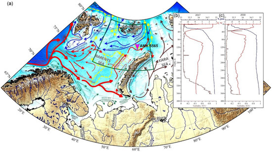
Figure 1.
Location of the mooring—Automatic Deep-Sea Sedimentary Observatory (station AMK-5565) and general directions of currents: (a) Red arrows—warm currents; blue arrows—cold currents, green arrows—coastal currents, yellow dashed arrows—subsurface (>100 m) currents, brown arrows—general circulation in the Kara Sea after [4,14,15]. Vertical profiles of temperature, salinity and turbidity before the deployment (b) and after the retrieval (c) of the ADOS. Green frame shows the position of Figure 2.
Marine phytoplankton is considered to be one of the tracers of changes in the environmental conditions, notably, light availability, temperature, water-column stability and salinity, since species distribution is strictly dependent on these environmental factors [16,17,18,19,20]. Over more than a century, comprehensive data have been accumulated on the composition of phytoplankton communities [19,21,22,23], remains of phytoplankton in the surface sediments [24,25,26,27,28,29] and in the Neogene, Pleistocene and Holocene sediments [19,24,25,26,30,31,32] of the Barents Sea.
One of the dominant phytoplankton groups in the Barents Sea are diatoms and dinoflagellates. The latter form cysts that are well-preserved in sediments during their life cycle. Dinoflagellate cysts are among the most studied components of the non-pollen palynomorph (NPP), which also includes green algae, acritarchs, copepod eggs, tintinnid loricae, etc. [33]. Despite numerous differences in feeding types within planktonic dinoflagellate, their cysts are represented in sediments mainly by phototrophic (light-dependent) and heterotrophic species (one possible factor is the presence of diatom algae and other phytoplankton [33,34]). The Barents Sea sediments are characterized by low concentrations of microfossils, and often their complete absence, associated mainly with the redistribution of fine-grained particles over the elements of the bottom relief and the dissolution of individual silica valves [35,36]. Although dinocyst cell walls contain dinosporin, which allows them to persist in the sediment [37] we still do not know enough about their distribution in the Arctic seas. Benthic resting cysts differ from the planktonic dinoflagellates they were produced from both morphologically and structurally [33]. In this regard, a detailed study of diatoms and NPP assemblage in the sinking material is necessary, as it provides a unique source of information on sedimentation conditions, and particularly on the influence of natural-climatic and biological processes.
Particle fluxes in the ocean are one of the main quantitative sedimentation parameters. This allows study of the dynamics of sedimentation processes, analysis of the transformation of sinking material during migration through the water column, and evaluation of the amount and composition of the matter accumulated at the bottom. Studying the annual particle flux and composition is of particular importance, as it provides information about the seasonal variability of sedimentation processes and seasonal dynamics of the structure and functioning of the epipelagic ecosystems [38,39,40,41].
The annual study of the settling matter with sediment traps in the northeastern part of the Barents Sea was performed for the first time. Most of the previous studies were concentrated in the central and western parts of the sea [42,43,44,45,46], as well as in the adjacent areas of the Arctic Ocean [47,48,49,50,51,52], and were limited to short-term deployments of sediment traps. Annual deployments were only carried out in the adjacent seas; in particular, in the Kara Sea [53,54] and in the central part of the Arctic Ocean [49,52] at a considerable distance from the location of this study.
At the nearest annual mooring in the Kara Sea, high fluxes were revealed in September and during the ice-cover season in February and April [54]. Formation of polynya is most likely one of the factors responsible for the increase in the vertical particle flux during the winter in that region.
This paper presents the results of a detailed study of diatoms, NPP, pollen and spores assemblages in the sinking material from a high-latitude mooring station. We attempt to reveal the features of the annual dynamics of diatoms’ and dinoflagellate cysts’ assemblages in the photic layer of the northeastern part of the Barents Sea under the harsh conditions influenced by low irradiance during the sea-ice covering period, dominance of southward currents, modern climate and the presence of the nepheloid layer. Over the past two decades three phenomena have been observed in the Barents Sea: upper-ocean warming, retreating sea-ice cover, and an increase of Atlantic water influence [55,56,57,58]. The main driver of interannual variability in SST is the variability of the Atlantic water temperature, which has increased significantly since 2005 [59]. Therefore, a special task was to find out whether the sinking material of the Eastern Barents Sea contains species of diatoms and dinoflagellate cysts, such as Coscinodiscus radiatus, C. perforatus, Shionodiscus oestrupii [25,60,61] and Operculodinium centrocarpum [62,63], which are indicators of the advection of transformed Atlantic waters into the Arctic seas.
2. Materials and Methods
The data for the study were obtained in the Eastern Barents Sea (East Barents Sea Depression) over the course of a year, from 9 August 2017 (cruise 68 of the R/V Akademik Mstislav Keldysh [64]) to 4 August 2018 (cruise 71 of the R/V Akademik Mstislav Keldysh [65]), using the Automatic Deep-Water Sedimentary Observatory (ADOS [66])—mooring with sediment trap) at the site of 77°59.933 N and 61°06.823 E at the sea depth of 370 m (Figure 1). The SBE 911plus CTD was used to study the water column during deployment and raising of the ADOS. Acoustic Doppler current profiler (ADCP) Teledyne RD Instruments DVS with a recording interval of 1 h was positioned 5 m above the trap to study the currents during the deployment period of the ADOS.
Sinking material was sampled with a sediment trap at 350 m depths to evaluate the flux reaching the bottom and contributing to the sediment formation. The deposited material was collected with the LOTOS-3 12-cup conical sediment trap with a sampling area of 0.5 m2 (produced by the Experimental Design Bureau of Oceanological Engineering, Russian Academy of Sciences) programmed for a temporal resolution of 30 days.
The cup samplers of the traps were filled with a HgCl2 solution (1% saturated solution) to avoid biological transformation of the sampled material. The salinity of the fixing solution was increased by adding NaCl to double the salinity of the seawater (~70 PSU) to prevent leaking of the fixing solution from the samplers. Each trap’s sample was prefiltered through a sieve with a mesh size of 1 mm to remove “swimmers” [41,54,67]. Particles >1 mm retained in the sieve were placed in a separate vial.
A total of 12 cups were used to collect settling sediments—one for each month during the year. The sedimentary material was filtered under 400 mbar vacuum through membrane nuclearpore filters (0.45 μm pore size and 47 mm filter diameter). The mass concentration was determined by weighing the filters with an accuracy of ±0.01 mg [41].
For elemental analysis, a CHNS EuroEa 3000 EuroVector elemental analyzer was used to measure particulate total carbon and total nitrogen. The analysis was performed by catalytic combustion, followed by packed column gas chromatographic separation with thermal conductivity detection. The analytical accuracy was 0.3–0.5 wt.%. Particulate total carbon (PTC) and particulate inorganic carbon (PIC) were measured with a Shimadzu TOC-L analyzer with SSM-5000A module. PIC was measured directly by coulometry, which is the measurement of CO2 following closed-system conversion of PIC to CO2 upon addition of phosphoric acid [39]. Particulate organic carbon (POC) was determined by the difference between PTC and PIC. The analytical accuracy was 1.0 wt.%.
The samples for diatom analysis were treated using standard preparation techniques [19] and then mounted on slides with Naphrax at the IO RAS. The sediments of the Barents Sea are characterized by low diatom concentrations, and sometimes their complete absence [36]. The amount of the sinking material obtained using the sediment trap and processed for diatom analysis is small. Therefore, we counted all valves contained in the studied sinking material. In most cases, 100 specimens were found in each sample, using an Axiostar Plus microscope (Carl Zeiss) (oil immersion CP-Apochromat lens, magnification 1000×, numerical aperture 1.25). Diatom identification was performed at the species’, varietal, or forma levels. Diatom total concentrations per gram of dry sediment (valves g−1) were calculated using the Battarbee method [68]. Then, based on the total mass flux data [69] and diatom concentrations, the average monthly number of diatom valves per m2 per day (diatom flux, valves m−2 day−1) was calculated.
The classification of diatoms is based on the system by Round F.E., Crawford R.M., Mann D.G. [70] with additions from later publications [71,72], as well as catalogs of genera and species of diatoms published in print and on the Internet: Fourtanier, Kociolek, [73], Kusber, Jahn, [74], Morphbank, [75], Diatoms of North America [76], AlgaeBase, [77].
Palynomorphs were extracted as per following the standard palynological techniques at the IO RAS [78] and concentrations were calculated using calibrated tablets of Lycopodium clavatum spores [79]. Dinoflagellate cysts were mainly identified on slides, with the help of an Axio Imager.A2 light microscope with EC “Plan-Neofluar” 400×, 1000× magnifications and N-Achroplan 630× magnification. Other organic-walled microfossils, such as pollen grains and spores, zooplankton remains (foraminifer linings, copepod eggs, tintinnid loricae), were examined at the same time. Because of the extremely low weights of the samples, we could only measure concentrations (specimens per g of dry sediment) to be counted. Dinocyst and Lycopodium spore counts in the whole sample ranged from less than 10 to ~200 and from 10 to ~120 specimens, respectively. Thus, for low-count samples [63] taken during the months with strong sea-ice cover, the statistical error can exceed 30% [79]. However, we believe that these data are still worthy of presentation due to the fact that our mooring station is located in a unique region where the sediment fluxes and abundance of palynomorphs are extremely low, and similar studies have never been conducted before. Similar to the diatoms, concentrations were subsequently converted to average monthly flux values (specimen’s m−2 day−1).
Dinoflagellate cyst taxonomy is in line with well-known systematic publications (Fensome et al. [80], Van Nieuwenhove et al. [81], Limoges et al. [82], Mertens et al. [83], etc.). The cysts of Polarella glacialis and cf. Biecheleria sp., which can be found mainly in the more recent sediments [18], were included in the dinocyst group due to the overall low content of dinocysts. Tintinnid loricae and ciliate cysts were identified based on Heikkilä et al. [18] and Dolan et al. [84].
Multivariate analyses were performed to extract the dominate factors of the diatoms and dinocysts fluxes variability in relation with environmental variables (sea-ice cover (SIC), solar radiation (Solar), POC and N flux) (Figure 2). A preliminary detrended canonical analysis (DCA) yielded a gradient of 2.8 for dinocyst and 3.0 SD for diatoms, indicating that redundancy analysis (RDA) can be used [85]. DCA and RDA were performed using the CANOCO software [Canonical Community Ordination: version 5.15 for Windows, 85]. Temperature and salinity were not included in the RDA, as their values from the World Ocean Atlas are highly averaged and are not available for all months during which fluxes were measured.
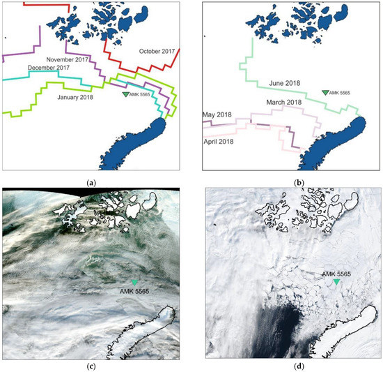
Figure 2.
Sea-ice cover boundaries according to the National Ice Center Arctic and Antarctic Sea Ice data [86,87]: (a) in October 2017–January 2018, when the sediment trap location was in close proximity to the sea-ice edge and (b) in March 2018–June 2018, when the sediment trap location was covered with sea ice. Satellite images show ice distribution: (c) 6 October 2017 and (d) 10 April 2017 (VIIRS instrument, [88]).
To assess the sea-ice conditions and ice concentration in the area of the trap deployment, we used data from the U.S. National Ice Center Arctic and Antarctic Sea Ice [86] and the Arctic and Antarctic Research Institute [87]. The 10.7 cm solar flux data were provided as a service by the National Research Council of Canada [89,90]. The radar system is operated at a frequency of 2800 MHz, that is a wavelength of 10.7 cm. The 10.7 cm solar flux is currently one of the best indices of solar activity, presented in “solar flux units”, (s.f.u.) [90,91].
Back trajectories of air masses were calculated using the HYSPLIT Trajectory Model [92,93] available from the READY website [94].
3. Results
3.1. Environmental Parameters at the Mooring Site
The temperature, salinity and turbidity profiles were recorded before the deployment and after the retrieval of the mooring (see Figure 1b,c). In August 2017, the temperature in the mixed layer was 2.50 °C; while salinity was 33.3 PSU. Deeper, down, to a depth of 40 m, there was a cold intermediate layer with a temperature decrease to −1.4 °C and salinity increase up to 34.3 PSU (cold and fresh Arctic waters). In the 40–100 m layer, the temperature increased to >1 °C, and salinity was up to 34.8 PSU (warm and salted subsurface Atlantic waters). In the deepest layer, the temperature gradually dropped to 0.1 °C, while the salinity varied slightly. Turbidity values remained practically unchanged to the depth of 280 m and increased up to 0.8 NTU in the near-bottom layer at 280–360 m depths. After the retrieval of the sediment trap (Figure 1c) in July 2018, the temperature in the mixed layer was lower than in August 2017 by about 1.8–2.0 °C, while salinity was slightly higher, increasing from 33.4 to 33.5 PSU. The temperature of the cold intermediate layer (16–40 m) decreased to −1.0 °C, and salinity increased to 34.5 PSU. Turbidity peaked up to 0.5 NTU at the depth of 34.6 m. In the 40–60 m layer, the temperature and salinity increased to 0.9 °C and 34.8 PSU, respectively. At a depth of 360 m, the salinity changes imperceptibly to 34.9 PSU from top to bottom. Temperature decreased gradually from 0.9 to −0.6 °C at the 60–290 m layer and then increased slowly to 0 °C at a depth of 365 m. Turbidity, except for the aforementioned peak, increased from top to bottom and reached maximum values (0.2–2.4 NTU) in the near-bottom layer at 310–365 m depths.
ADCP data recorded mainly currents directed to the southwest in the sediment trap location. The maximum current velocity (16 cm per second) was registered in the southwesterly direction in December 2017 and January 2018 (Figure 3).
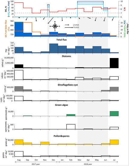
Figure 3.
Annual data from AMK-5565 ADOS: Sea-ice cover (concentration in %), C:N and monthly averaged current vectors; particulate organic carbon (POC) and solar flux; total mass flux; overall concentrations (filled silhouettes) and fluxes (empty silhouettes) of diatoms, dinoflagellate cysts, green algae, pollen and spores. Light gray rectangles mark the ice-covered season (SIC > 50%).
3.2. Monthly Changes of Sea-Ice Covers and Seasonal Cycle of Solar Light Availability
An analysis of the sea-ice cover maps (Figure 2a,b) of the Barents Sea showed that from August to October 2017, the East Barents Sea depression in the sediment trap location was ice-free. In November, the sediment trap was located right on the border of the sea-ice cover, the thickness of which varied from 10 to 30 cm. From December 2017 to February 2018, the study site was free of sea ice, but was in close proximity to its edge. During March, April, May and June 2018, the study area was covered with sea ice, the concentration of which was 70–100% and the thickness was from 30 to 200 cm. In July 2018, the study area was ice-free [86,87].
Analysis of the monthly climatic time series of solar light flux (10.7 cm) showed that over the mooring period there was an increase in solar activity in August–November 2017, February 2018 and from April to June 2018 (Figure 3).
3.3. Mass, Carbon and Total Fluxes
The seasonal variability of total mass, total carbon, POC fluxes, C:N were investigated in relation to the general fluxes of diatoms, dinocysts, green algae, pollen and spores and other NPP (Figure 3 and Table S1). Seasonal ice cover and solar flux were also considered for interpretation. Due to low carbonate content, the fluxes of total and organic carbon are almost identical.
The high total mass and carbon fluxes were measured in August 2017 (187 mg m−2 day−1 and 32.8 mg C m−2 day−1). From September to November 2017 and in July 2018, the total mass fluxes were reduced to 22–53 mg m−2 day−1, while carbon fluxes were reduced to 2–8 mg C m−2 day−1. From December 2017 to May 2018, the total mass fluxes were highest (up to 293 mg m−2 day−1 in winter season), while maximum current velocity (up to 16 cm/s) were recorded in the southwesterly direction. Carbon fluxes during the period varied between 5–10 mg C m−2 day−1. It is interesting to note that the strong seasonal ice cover from March to June 2018 had practically no effect on the total fluxes. Nevertheless, annual C:N ratio over 7 indicates an ongoing particulate terrigenous matter supply. Therefore, it seems unfeasible to separate vertical and lateral fluxes.
The diatoms and palynomorphs fluxes did not always coincide with total mass due to the strong influence of terrigenous matter. The maximum fluxes of the diatoms, dinocysts as well as pollen and spores are observed in August 2017 (640.9 × 10³ valves m−2 day−1, 90 × 103 species m−2 day−1, 16 × 103 grans m−2 day−1) and June–July 2018 (216.9 × 10³ valves m−2 day−1, 16 × 103 species m−2 day−1, 3 × 10³ grains m−2 day−1) after the ice cover breakup. The green algae fluxes were relatively high in February and July 2018 (up to 860 specimens m−2 day−1).
3.4. Diatom Fluxes and Assemblages
Diatom assemblages were analyzed in all 12 samples. The diatom concentrations range from the minimum value of 153.5 × 10³ valves g−1 in February 2018 to the maximum of 9626.1 × 103 valves g−1 in July 2018 (Figure 3 and Table S1). The average monthly number of diatom valves per m2 per day was the highest in August 2017 and equaled 640.9 × 10³ valves m−2 day−1. Local peaks were recorded in March and July 2018, when the average monthly number of diatom valves per m2 per day was 162.4 and 216.9 × 10³ valves m−2 day−1, respectively.
The taxonomic diversity of diatoms in the sinking material is rather high for this region [36,95], with approximately 29 diatom taxa identified, of which 21 were marine and brackish, while the eight remaining ones were freshwater species (Figure 4 and Figure 5. Table S1).
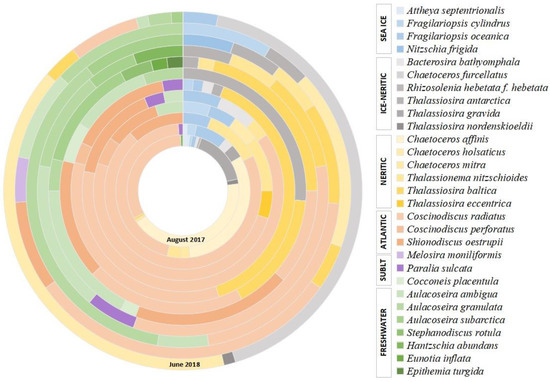
Figure 4.
Diatom assemblage’s composition (%) in the sinking material of the East Barents Sea Depression. “SUBLT” means sublittoral.
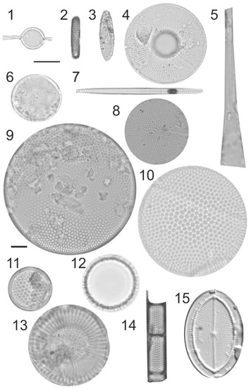
Figure 5.
Photomicrographs (bright-field images) of diatoms recovered from 2017 to 2018 sediment trap moorings in the Barents Sea, taken with an Axiocam 305 color microscope camera mounted on a Zeiss Axio Imager.A2 light microscope with EC “Plan-Neofluar” 100x/1.30 Oil objectiv. (1). Attheya septentrionalis, August 2017. (2). Fragilariopsis cylindrus, September 2017. (3). Fragilariopsis oceanica, September 2017. (4). Bacterosira bathyomphala, September 2017. (5). Rhizosolenia hebetata f. hebetata, August 2017. (6). Thalassiosira nordenskioeldii, August 2017. (7). Thalassionema nitzschioides, October 2017. (8). Thalassiosira eccentrica, November 2017. (9). Coscinodiscus perforatus, January 2018. (10). Coscinodiscus radiatus, August 2017. (11). Shionodiscus oestrupii, March 2018. (12). Paralia sulcata, April 2018. (13). Stephanodiscus rotula, March 2018. (14). Aulacoseira granulata, May, 2018. (15). Cocconeis placentula, March 2018. Scale bar 10 µm.
Among the former, neritic species predominate (55.5–97.7%). Approximately half of them are ice-neritic species (up to 45%) represented by Thalassiosira nordenskieldii, Th. gravida, Th. antarctica, Bacterosira bathyomphala, Rhizosolenia hebetata f. hebetata, Chaetoceros furcellatus, which develop in the plankton of the marginal ice zone, often at close to zero or negative surface water temperatures [19,96]. Indicators of the Atlantic waters advection into the western Arctic seas, such as relatively warm-water Coscinodiscus radiatus, C. perforatus and Shionodiscus oestrupii [25,60], were also found in great abundance (up to 82%, 1112.7 × 103 valves g−1 and 210 × 103 valves m−2 day−1) and among them, Coscinodiscus radiatus constantly dominated. Sublittoral meroplanktonic Paralia sulcata and Melosira moniliformis are rare (0–5.8%). The proportions of planktonic freshwater species Aulacoseira ambigua, A. granulata, A. subarctica, Stephanodiscus rotula and benthic Eunotia inflata, Epithemia turgida, Hantzschia abundans in sinking material’s diatom assemblages vary from 0 to 52.6%. Sea-ice species, whose lifecycle is associated with the sea ice [25,97,98] are represented by single valves of Fragilariopsis cylindrus, F. oceanica and Attheya septentrionalis and Nitzschia frigida and their proportions do not exceed 11%.
The sediment trap was deployed in August of 2017. Total diatom concentration of sinking material in this period was 3430.8 × 103 valves g−1. Diatom flux value was 640.9 × 10³ valves m−2 day−1, the highest for the entire accumulation period. The composition of diatom assemblages in the August 2017 sinking material is dominated by marine planktonic neritic species, mainly Coscinodiscus radiatus and Chaetoceros affinis (97.3%). The complex of ice-neritic species is widely represented (18.9%) by Bacterosira bathyomphala, Rhizosolenia hebetata f. hebetata, Thalassiosira gravida and Th. nordenskioeldii. The proportion of sea-ice species, namely Attheya septentrionalis, Fragilariopsis cylindrus, F. oceanica, is 4.05%. Freshwater species are represented by single valves of Hantzschia abundans (0.68%, 4.3 × 10³ valves m−2 day−1; Figure 5 and Figure 6).
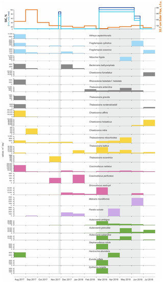
Figure 6.
Annual diatom fluxes in the East Barents Sea Depression. Legend: sea-ice diatom species—blue, ice-neritic species—grey, neritic species—yellow, Atlantic species—magenta, sublittoral species—purple, freshwater species—green. The top shows the sea-ice cover (concentration in %), and solar flux, light gray rectangles mark the ice-covered season (SIC > 50%).
In the sinking material accumulated in the autumn of 2017, diatom concentrations consistently decrease from 561.4 × 10³ valves g−1 to 311.1 × 10³ valves g−1. Diatom fluxes were recorded at 29.8, 10.5, 15.5 × 10³ valves m−2 day−1 in the September, October and November sinking material, respectively. Diatom composition is represented by 8 neritic, 2 ice-neritic, 3 sea ice, 1 sublittoral and 1 freshwater species. Planktonic neritic species dominate (85–94%) and among them Coscinodiscus radiatus (46–70%; 7–13 × 103 valves m−2 day−1). Ice-neritic Bacterosira bathyomphala and Thalassiosira gravida species (up to 5.5%) were only found in the September sinking material.
The proportion of sea-ice species Fragilariopsis cylindrus, F. oceanica and Attheya septentrionalis varies from 6 to 11%. Freshwater species were only found in the November sinking material and are represented by single valves of Aulacoseira ambiqua (0.9 × 10³ valves m−2 day−1). The proportion of these species is low and does not exceed 5%.
In the winter of 2017–2018, the total diatom concentrations were the lowest during the year, decreasing from 210.7 × 10³ valves g−1 to 153.5 × 10³ valves g−1. At the same time, the relative abundance of Coscinodiscus radiatus in the diatom assemblages, which is an indicator of the Atlantic waters advection into the western Arctic seas [25,60], decreased from 64 to 23%. The winter diatom flux values varied from 61.7 to 21.6 × 10³ valves m−2 day−1, consistently decreasing by three times from December to February and were generally higher than those in autumn. Ice-neritic species Thalassiosira antarctica appeared in the sinking material, which accumulated in January and February. The other ice-neritic species Bacterosira bathyomphala was found in the sinking material that accumulated in December and January (3.9 and 0.7 × 10³ valves m−2 day−1), and in other months of the year Bacterosira bathyomphala is not characteristic for the diatom composition, while Th. antarctica was found in the sinking material up until June. Neritic species were fairly abundant, falling below 80% only in February due to the appearance of a large number of freshwater species (21%; 32.3 × 10³ valves g−1; 5.5 × 10³ valves m−2 day−1), including freshwater plankton species Aulacoseira ambiqua and A. granulosa (15.8%). Sea-ice species were only found in the sinking material of the first two winter months and their proportion almost halved during this period (6.25–2.98%).
In the sinking material accumulated during the spring months of 2018, the concentrations of diatoms increased up to 753.5 × 10³ valves g−1, while diatom flux varied from 162.4 × 10³ valves m−2 day−1 in March to 63.9 × 10³ valves m−2 day−1 in April and to 108.7 × 10³ valves m−2 day−1 in May. Planktonic neritic species Coscinodiscus radiatus, Thalassiosira baltica, Shionodiscus oestrupii, Thalassionema nitzschioides dominated constantly in diatom assemblages. However, the content of marine planktonic neritic species did not exceed 60% (55.8–42.7%) and was the lowest in May. Sea ice species were only found in small numbers (5.3%; 9.8 × 10³ valves m−2 day−1), and the proportion of ice-neritic species increased from March to May (1.9–5.3%). The freshwater species proportion was the highest for the whole year and was 38.8–52.6%. The greatest diversity of freshwater species was recorded in the March sinking material. Most species are represented by river plankton Aulacoseira subarctica, A. ambigua, Stephanodiscus rotula, usually entering shelf seas with rivers runoff, as well as benthic freshwater species Eunotia inflata, Hantzschia abundans and Cocconeis placentula. The latter is found both in freshwater reservoirs and in the littoral of the seas.
In the first two summer months of 2018 the abundance of diatoms in the sinking material increased, reaching 9.626 × 10³ valves g−1 in July. Diatom flux varied from 61.3 and 216.9 × 10³ valves m−2 day−1. The proportion of marine planktonic neritic species increased (65–92%) at the expense of Chaetoceros holsaticus and Thalassiosira baltica. The proportion of ice-neritic species represented by Chaetoceros furcellatus, Thalassiosira antarctica and Th. nordenskieldii increased significantly. The latter is particularly characteristic for the sinking material of the summer months, namely July 2018 and August 2017. Marine planktonic ice-neritic species Chaetoceros furcellatus, Thalassiosira nordenskioeldii, Rhizosolenia hebetata f. hebetata, and cold-water neritic Ch. holsaticus dominated in diatom assemblages. Sea-ice species Fragilariopsis oceanica, F. cylindrus (8.7–3.15%; 7.2 × 10³ valves m−2 day−1) were found singly. In June and July, the number of freshwater species reduced significantly—down to 21.7% and 4.2%, respectively, and they were only represented by river planktonic Aulacoseira sp.
3.5. NPP, Pollen and Spores Fluxes and Assemblages
The NPP assemblages in annual sediment trap samples were mainly represented by dinoflagellate cyst (avg. 113.2 × 10³ cyst g−1), green algae (avg. 2.18 × 10³ specimen’s g−1), tintinnid loricae and cysts (avg. 1.48 × 10³ specimen’s g−1). Pollen and spore concentrations (avg. 27.8 × 10³ grains g−1) were comparable to those of dinocysts (Figure 3).
The average dinocyst flux was 12.4 × 10³ cysts (min 344 cysts m−2 day−1, max 90.0 × 10³ cysts m−2 day−1). The significant contribution of normally poorly preserved cysts of Polarella glacialis and cf. Biecheleria sp. in the sediments increased the fluxes mainly in August 2017 and July 2018 (Figure 6). Dinocyst flux has clear seasonal dynamics, resulting in the change of the main dominants in the associations through the year. Due to the high-latitude location of the station, seasonal variability occurs with an offset in relation to calendar seasons. The “warm” season includes July, August and September, while the “cold” season lasts from March to June and is characterized by a stable seasonal ice cover.
In total, 13 taxa of dinoflagellate cysts typical of the Barents Sea were identified in trap samples (Figure 7 and Figure 8; Table S1). Heterotrophic species, which are the most common group in this region [28,62,99,100,101], are represented by Echinidinium karaense, Islandinium minutum subsp. minutum, Islandinium? cezare and Brigantedinium spp. These species normally dominate in the cold Arctic surface water mass distribution area with strong seasonal ice cover [102,103]. The cosmopolitan autotrophic species Operculodinium centrocarpum (with short processes and its Arctic morphotype), Spiniferites ramosus, Spiniferites elongatus, Bitectatodinium tepikiense and Pentapharsodinium dalei indicate the influence of the Atlantic waters in the Western Arctic [102,103,104]. The cysts of Polarella glacialis and cf. Biecheleria sp. made the greatest contribution to the NPP associations after the ice season. Polarella glacialis and its cysts were found in sea-ice brine channels in the Arctic and Antarctic [105,106,107]. According to Hegseth and von Quillfeldt [108], in the western part of the Barents Sea, these bipolar dinoflagellates inhabited the ice, both as vegetative cells and cysts. They suggest that the algae are pulled out of the ice and begin to sink in late spring, when melting begins [108]. The other thin-walled cyst in the annual trap association is the specimen of cf. Biecheleria sp. It was associated with cysts of Biecheleria baltica described in the brackish northern Baltic Sea [109]. Both types of cysts are also described in the sediment trap and surface sediments of Hudson Bay [18,109].
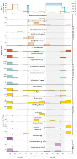
Figure 7.
Annual dinoflagellate cyst fluxes at the mooring station of AMK-5565 ADOS. Phototrophic taxa are indicated in orange and heterotrophic in blue, while darker shades of orange and blue indicate the proportion of cysts found with cell content. Pollen and spore flux is shown in yellow and organic-walled remains flux in purple. The top shows the sea-ice cover (concentration in %), and solar flux, light gray rectangles mark the ice-covered season (SIC > 50%).
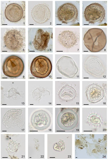
Figure 8.
Photomicrographs (bright-field images) of dinoflagellate cysts and NPP recovered from 2017 to 2018 sediment trap moorings in the Barents Sea, taken with an Axiocam 305 color microscope camera mounted on a Zeiss Axio Imager.A2 light microscope with N-Achroplan 10x/0.25 (image 22, 24), EC “Plan-Neofluar” 40x/0.75 (images 1–17, 23), N-Achroplan 63x/0.85 (images 18–21) objectives. Black scale bar is 10 μm. (1). Islandinium minutum subsp. minutum, optical section, August 2017. (2). Islandinium sp., optical section, March 2018. (3–6). Three Echinidinium karaense, high and mid-focus, (3,4) August 2017, optical section, (5) November 2017 and (6) August 2017. 7. Echinidinium sp., optical section, May 2018. (8–10). Two Brigantedinium spp., (8) optical section, (9,10) high and mid-focus, August 2017. (11,12). Bitectatodinium tepikiense, high and low-focus, October 2017. (13). Spiniferites ramosus, optical section, March 2018. (14,15). Operculodinium centrocarpum, optical section, (14) December 2017 and (15) January 2018. (16,17). Operculodinium centrocarpum short processes, optical section, (16) January 2018 and (17) March 2018. (18,19). cf. Biecheleria sp., optical section, (18) August 2017 and (19) September 2017. (20–22). Polarella glacialis, optical section, (20,21) August 2017 and (22) March 2018. (23). Botryococcus cf. braunii, February 2018. (24). Parafavella sp. lorica, August 2017.
Therefore, there are two main groups distinguished mainly by the type of feeding and relation to seasonal ice cover. The first group includes poorly preserved autotrophic cysts of Polarella glacialis and cf. Biecheleria sp., whose fluxes increase sharply immediately after the melting of seasonal ice in June, July 2018 and August 2017. Some increase in their fluxes (up to 8.2 cysts m−2 day−1) was observed even after a brief approach of the ice field edge in late November 2017 and continued until January 2018. Some fluxes of heterotrophic dinoflagellate cysts observed during and just after the ice season (June 2018) are E. karaense and I. minutum subsp. minutum, while Brigantedinium spp. and maximum fluxes (up to 14.6 cysts m−2 day−1) of E. karaense, I. minutum subsp. minutum and I.? cezare were found also during the summer months in open water (August–September 2017).
Cyst fluxes of autotrophic dinoflagellates (P. dalei, O. centrocarpum, B. tepikiense S. ramosus, and S. elongatus), which belong to the second group, were common from December 2017 to February 2018. The lowest total fluxes were responsible for the low content of dinocysts and other palynomorphs in the autumn period from the end of September to November 2017 and corresponded to the polar night season. During almost all of the ice season in early spring from March to May, autotrophic dinocyst species occurred sporadically, while heterotrophic species were completely absent until June 2018 (Figure 7).
The green algae fluxes (ca. 860 specimens m−2 day−1) are only half those of dinocysts and occur mostly in September 2017, February, and July 2018. The green algae diversity is presented by Botryococcus cf. braunii and Pediastrum boryanum.
Pollen fluxes are probably associated with the wind transport during the high-latitude seasonal bloom [110] and reach their peaks from June to August 2017 (up to 16 × 103 grains m−2 day−1). In June–July 2018, shrubs (Betula nana) with Lycopodiacea and Sphagnum spores were present, and were then replaced by conifer tree pollen (Pinus and Picea). Thus, the summer pollen fluxes may be associated with wind influxes from the northern parts of European Russia (Figure 9a,c). However, the second increase in fluxes during the autumn–winter season from November to February with Pinus and Picea pollen occurs along with shrubs, single herbs and mosses. The area of the winter wind pollen inflow does not extend beyond the boundaries of the seasonal snow cover zone (Figure 9b), thus, water masses and re-suspension of deposited matter are the main source of pollen and spores.
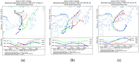
Figure 9.
Typical backward trajectories by month: (a) in August 2017, (b) in February 2018 and (c) July 2018.
Other organic-walled remains (ciliate loricae and cysts, copepod eggs) fluxes are timed to August 2018 (up to 1.4 × 10³ specimens m−2 day−1), when the maximum fluxes of dinocysts were recorded. Moreover, Acanthostomella sp. lorica was found in May 2018 during the strong seasonal ice-cover along with the arctic-boreal genera Parafavella sp. lorica (Figure 7).
3.6. Relation of Diatoms and Dinocyst Species to Light Availability, SIC, POC and N fluxes
Redundancy analysis provides additional insight into the relationship between the annual distribution of diatoms and dinocysts and environmental parameters. The dinocyst RDA results showed that the first two axes explain, respectively, 41.05% and 12.2% of the total variance (Table 1). The POC, N and solar fluxes correlate with the first axis (R2 = 0.6089, 0.4782 and 0.6539 respectively), whereas the SIC is linked to axis 2 (R2 = 0.8181; Table 2). Axis RDA1 shows the best positive correlations with Islandinium? cezare (97.96%), Brigantedinium spp. (83.19%), Islandinium minutum subsp. minutum (78.43%) and Echinidinium karaense (65.81%; Figure 10). The RDA triplot (Figure 10) shows that, in general, cyst fluxes are negatively correlated or unrelated to the sea-ice concentrations. The cysts of cf. Biecheleria sp. (72.05%) and Polarella glacialis (47.87%) have shown the strongest negative relation with SIC. Other autotrophic dinocyst species also fit to the second axis (RDA2) the least, while heterotrophic species showed a better relation to it.

Table 1.
Results of redundancy analysis.
Table 2.
Coefficient of correlation between environmental parameters and the scores of the two first axes of redundancy analysis. Parameter abbreviations are shown below Figure 10. Bold numbers correspond to parameters which are best correlated to axes.
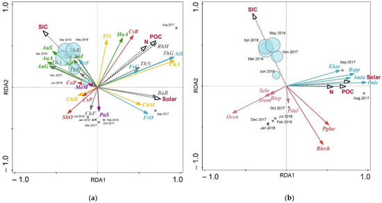
Figure 10.
Correlation triplot of redundancy analysis (RDA) of diatom and (a) dinocyst (b) fluxes displaying the species responses to sea-ice concentration (SIC), POC, N and solar fluxes (Solar). Months when the sediment trap location was covered with sea ice are marked in light blue circles (size matches the concentration, while crosses correspond to SIC = 0%). Sea-ice diatom species are marked blue, ice-neritic—grey, neritic—yellow, Atlantic—red, sublittoral—purple, freshwater—green. Autotrophic dinocysts are marked pink, autotrophic sea-ice dinocysts—red, heterotrophic—blue.
The diatoms RDA results show that the first ordination axis (RDA1) explains only 27.54% of the variance and the second axis (RDA2) only 10.8% (Table 1). Similar to the dinocysts case, a positive correlation with the first axis POC (R2 = 0.6391), N (R2 = 0.5344) and solar (R2 = 0.6912) fluxes was established, while RDA2 showed a positive correlation with SIC (R2 = 0.5637) and POC (R2 = 0.4647; Table 2). The best fit for the first axis are the Attheya septentrionalis (92.17%), Chaetoceros affinis (92.77%), Thalassiosira gravida (92.03%) species, ordinated on the positive side, while Aulacoseira ambiqua (60.68%), A. granulata (58.14%), A. subarctica (54.41%) are ordinated on the negative side. Coscinodiscus radiatus show the best fit (62.81%) for the second ordination axis in addition to Thalassionema nitzschioides (59.53%), Hantzschia abundans (57.02%).
4. Discussion
This study presents the results of annual continuous measurements of microfossils fluxes (diatoms, dinoflagellate cyst and other palynomorpths) in a high-latitude marine sedimentary system with seasonal ice cover. First, the unique location of the station at the point of interaction of several types of water masses affects the species assemblages in general, and its annual variability is mainly due to the irradiance of the photic layer and the duration of sea ice cover period. Second, the ongoing Atlantification of the Barents Sea [13,59] has resulted in the penetration of relatively warm Atlantic species not being limited to the summer season, but continuing throughout the year. The analysis of high-latitude data under conditions of low values of sediment fluxes imposes significant limitations on the use of traditional research methods.
4.1. The Specifics of Obtaining and Interpreting High-Latitude Sediment Trap Data
Previously, analysis of satellite data and the results of a short-term deployment of sediment traps in the Barents Sea showed that the vertical distribution of chlorophyll “a” fluxes, as an indicator of the settling of freshly produced particles (flocculent phytodetritus), corresponds to the temporal variability of chlorophyll “a” concentrations in the surface layer of the sea [46]. Thus, the minimum level of chlorophyll flux at the 100 m layer corresponded to the minimum level of chlorophyll concentrations in the surface layer of the sea during the collection of the matter by traps. At the same time, the maximum level of chlorophyll “a” flux in the 200 m layer corresponded to the maximum level of chlorophyll “a” concentration on the sea surface 8 days before the traps were deployed. Therefore, the sedimentation of planktonic cells from the upper active layer to a depth of 200 m can take about 8 days. By extrapolation, it can be calculated that the particles can arrive at a depth of 345–350 m with a delay of about 14 days. The microalgae found in the sediment matter were part of the phytoplankton two weeks earlier. In addition to the physical factor of delayed signal arrival from the planktonic assemblage to the seabed, its initial composition contributes greatly to the disposal of microalgae remains.
The annual composition of microfossils is determined by the unique high-latitude position of the station, which is located at the site of interaction between the northern cold Arctic water mass, the relatively warm and salty transformed southern Barents Sea mass, and the subsurface North Atlantic mass entering the St. Anna from the continental slope (Figure 1). The diatom assemblages of sinking material include 29 species and only reflect a relatively small sample of the Barents Sea diatom plankton diversity, which includes more than 100 taxa [13,25,36,111,112]. At the same time, the number of diatom species in the bottom sediments’ surface layer does not exceed 23 and the distribution of planktonic diatom species on the surface of the sea bottom strictly corresponds to their modern ranges. Most of the ice-neritic and sea-ice diatoms appear during a short period of under two weeks [25,36]. A study of the western and southwestern parts of the Barents Sea revealed 22 to 25 dinocysts species in the surface sediments [26,27,28,102,103,113]. At the same time, at our mooring station located in the north-east of the Barents Sea, only 13 species were observed during the year. With more than 125 planktonic species observed in the Barents Sea [114], only about 10–20% of dinoflagellates can be found in sediments as resting cysts, which does not contradict the commonly accepted data on the response of planktonic communities [33,115,116]. Thus, the depleted composition of microfossils in the annual sediment trap is explained by its high-latitude location and low fluxes of organic matter.
Turbidity values before deployment and after the retrieval of the mooring (Figure 1b,c) assume that sinking material has an admix of sea-bed-derived organic matter. This indicates a prominent role of resettled material, causing the need to be cautious in interpreting the data. The presence of sublittoral diatoms in the sinking material of this deep-water region of the Barents Sea (370 m) can only be associated with their transportation by bottom currents. We noted low counts of diatoms and dinoflagellates and low percentage of cysts with live contents, mostly overlapping microfossil flux peaks with general fluxes, and the appearance of pollen and spore fluxes outside the vegetation season from October to February 2017. Similar problems have also been noted by other researchers of sediment traps [18,116,117]. Furthermore, due to the harsh arctic environmental conditions for planktonic diatoms and dinoflagellates in the Barents Sea and the structures of diatom cells, which dissolve before reaching the bottom under the conditions of silicic acid deficiency [25,36,118,119], the Barents Sea sediments are characterized by low concentrations of microfossils, and often their complete absence. On top of that, in many cases, the phytoplankton biomass fails to accumulate due to an extensive grazing by zooplankton [120]. The studied material also lacks theca of dinoflagellate, which may be due to extremely low amounts of sinking material and collection of re-suspended sediments from the seafloor.
4.2. The Role of Sea-Ice Cover and Light Availability
From March to May 2018, the study area was covered with sea ice (SIC = 100%), and the only sediment trap deployed there allowed the obtaining of unique data on the features of sedimentation and the seasonal microfossils composition.
Sea-ice diatoms are practically absent in the sediments of March, April and May 2018 (Figure 6), only single valves of Nitzschia frigida are found in the May sediment matter. This is probably due to the fact that sea-ice diatoms did not enter the sinking material during the ice cover period, and began to come in only once the ice began to melt with a delay of at least two weeks due to the sink-factor. The flux of ice-neritic species T. antarctica is quite large, which is probably because of the proximity to the ice edge. T. antarctica is one of the dominant species in the marginal ice zone of the Barents Sea during the phytoplankton spring bloom [95].
The dinoflagellate cyst flux during the months with strong SIC is practically negligible (Figure 3 and Figure 7). The exceptions are single cosmopolitan dinocysts probably re-suspended from sediments. Nevertheless, some of them are represented by O. centrocarpum cysts with live content. When SIC decreases to 50%, early spring bloom is observed in dinocyst associations, starting in the sea-ice brine channels and peaking at the ice margin in July 2018. There is a change in the dominant cyst species from sea-ice autotrophic species Polarella glacialis and heterotrophic I. minutum subsp. minutum, E. karaense to the autotrophic cf. Biecheleria sp. and O. centrocarpum. Similar to Hudson Bay [18], there is some displacement in peaks Polarella glacialis and cf. Biecheleria sp., since the former species is an ice dweller and the latter prefers under-ice blooming. The time lag between the entry of these species from the ice into the water and their subsequent settling is clearly reflected in the RDA results, where the SIC contrasted with the presence of Polarella glacialis and cf. Biecheleria sp. cysts in the sediment trap matter.
Maximum values of diatom concentrations in July 2018 (Figure 3) are apparently related to the spring peak of blooming, which occurs in the Barents Sea in June–late July and is associated with the process of ice melting and the formation of a marginal zone enriched with nutrients—Si, P, N [13]. The retreat of the sea-ice cover edge is accompanied by phytoplankton bloom. Taking into account the fact that the sedimentation of the material occurs after two weeks, the maximum concentrations of diatoms in the composition of phytoplankton apparently were in mid-June. As part of diatom assemblages, sea-ice and ice-neritic species (Fragilariopsis oceanica, Fr. cylindrus, Thalassiosira nordenskioeldii, T. antarctica) appear in large numbers, which is characteristic of the spring phytoplankton of the Barents Sea.
From late summer to early autumn (August–September 2017), when the ice margin was farthest to the north of the station, heterotrophic cosmopolitan species Brigantedinium spp. dominated, even though fluxes of autotrophic ice species were still high possibly due to both vertical and lateral transport. One of the most favorable light and nutrient conditions during the “polar summer” led to diatom bloom and provided unlimited access to food for heterotrophs. However, from October 2017 to February 2018, autotrophic dinocyst species began to dominate the assemblages, which serves as an indicator of ice-free open-water conditions.
Freshwater diatom species appeared in large abundance in March 2018 and remained in fairly high proportions until July 2018. Since river planktonic species show a negative correlation with the RDA1 and a weakly positive correlation with the RDA2 (Figure 10), we assume that their appearance in the sinking material accumulating from March 2018 to July 2018 is associated with the thawing of sea ice. The source of freshwater diatoms (Figure 6) in sea ice is freshwater streams on Franz Josef Land. This is also confirmed by the maximum fluxes of freshwater algae in July 2018. The contributions of pollen and spores of terrestrial plants depend mainly on the direction of the wind during the blooming season and on their transport with seasonal ice during the winter months.
Thus, the main factors responsible for changes in the seasonal assemblages of both diatoms and dinocysts are seasonal ice cover and irradiance, which are also indirectly related to the temperature and salinity of water masses, their stratification, amount of nutrients, etc.
4.3. The Influx of Relatively Warm-Water Species as A Result of the Barents Sea Atlantification
The Barents Sea is a “hot spot” for Arctic climate change, with significant interannual variability in the ice extent and an overall northward retreat of the ice edge observed over the past two decades [55,56,57,58]. One of the reasons for this is the increased influence of the Atlantic water in the region termed the “Atlantification” of the Arctic Ocean [121,122].
Indicators of the Atlantic waters advection into the western Arctic seas in the diatom (Coscinodiscus radiatus, C. perforates and Shionodiscus oestrupii) and autotrophic dinocyst (mainly Operculodinium centrocarpum) communities observed in the annual sinking material indicates the penetration of transformed Atlantic waters into this zone. It should be noted that high latitudes are undoubtedly sterile areas of eviction [123], where the cells of these algae are carried by currents and cannot develop. The transformed Atlantic waters enter the Eastern Barents Sea from the south with the continuation of the North Atlantic Current, and from the north with subsurface (>100 m) currents, which are probably passing through the St. Anna Trough [2,124]. In addition to diatoms and dinoflagetate cysts, another indicator of the Atlantic waters (namely, the cold-water coccolithophore Coccolithus pelagicus) was found up to 80° N in the plankton of the Barents Sea [13]. According to our data, regardless of the direction of the inflow, the transformed North Atlantic waters from mid-2017 to mid-2018 brought in the relatively warm microalgae species even during the winter and spring (with stable ice cover) seasons. This also aligns well with the previous investigations of spatiotemporal heat budgets [58], that show the Atlantic water penetration pathways and the increasing influence of Atlantification on the Barents Sea up to 80° N, which results in the significant warming of the water column.
5. Conclusions
Here, we discussed the annual diatom and NPP assemblages’ production, composition and flux in the northeastern part of the Barents Sea, formed under low irradiance of the photic layer during the sea-ice covering period, dominance of southward currents, modern climate changes and nepheloid layer conditions.
The main factors of seasonal variability of microfossils composition are the seasonal ice cover and irradiance. The inflow of sea-ice diatoms and dinocyst into the sinking material was practically negligible during the ice cover period, and began only with the onset of sea ice melting with probably a 1–2 weeks delay. Maximum values of diatom concentrations in July 2018 correspond to the spring bloom peak, which occurred in the Barents Sea in June–late July and were associated with the process of ice melting. High dinocyst fluxes in July were also associated with the melting of seasonal ice cover, while the maximum values of heterotrophic species fluxes in August were probably associated with their feeding.
Diatoms and dinocysts indicate the advection of the Atlantic waters into the Barents Sea up to 80°N. According to the microalgae analysis during the deployment of the sediment traps from mid-2017 to mid-2018, the inflow of these waters did not stop even in the winter months and during the stable ice cover from May to June 2018, due to the ongoing Atlantification of the Barents Sea [13,59].
The revealed features of diatoms and non-pollen palynomorphs assemblages in the sinking material of the northeastern part of the Barents Sea will serve as a methodological basis for Holocene paleoreconstructions, including the Atlantic waters advection into the Arctic Ocean, sea-ice cover and freshwater runoff.
Supplementary Materials
The following are available online at https://www.mdpi.com/article/10.3390/geosciences13010001/s1, Table S1: Lithological, geochemical and micropaleontological data from the annual sedimentation trap AMK-5565.
Author Contributions
Conceptualization, E.A. and E.N.; methodology, E.A., E.N. and M.K.; validation, M.K., investigation, E.A., E.N., A.K. and M.K; data curation, A.N. and M.K.; writing—original draft preparation, E.A., E.N., A.K. and A.N; visualization, E.A., E.N., A.K. and A.B.; organization, M.K., A.N. and A.K., field work, M.K., A.N., A.K. and A.B. All authors have read and agreed to the published version of the manuscript.
Funding
The study and the article were funded through a grant of the Ministry of Science and Higher Education of the Russian Federation (grant no. 075-15-2021-934) “Study of anthropogenic and natural factors of changes in the composition of air and environmental objects in Siberia and the Russian sector of the Arctic in conditions of rapid climate change using unique scientific facility Tu-134 Optik Flying Laboratory”. Field studies were supported by the state assignment of the Shirshov Institute of Oceanology RAS (no. FMWE-2021-0006).
Institutional Review Board Statement
Not applicable.
Informed Consent Statement
Not applicable.
Data Availability Statement
Not applicable.
Acknowledgments
The authors are grateful to Yelena Polyakova (MSU) for her invaluable advice and diatom atlases and Sergey Pisarev (IO RAS) for his consultations on hydrology conditions. We would also like to thank Elena Kudryavtseva (IO RAS) for her assistance in CN analysis. We also acknowledge the crew of the R/V Akademik Mstislav Keldysh. The authors gratefully acknowledge the NOAA Air Resources Laboratory (ARL) for the provision of the HYSPLIT transport and dispersion model and the READY website (https://www.ready.noaa.gov (accessed on 21 October 2022)) used in this publication.
Conflicts of Interest
The authors declare no conflict of interest.
References
- Sakshaug, E. Biomass and productivity distributions and their variability in the Barents Sea. ICES J. Mar. Sci. 1997, 54, 341–350. [Google Scholar] [CrossRef]
- Schauer, U.; Loeng, H.; Rudels, B.; Ozhigin, V.K.; Dieck, W. Atlantic water Flow through the Barents and Kara Seas. Deep-Sea Res. Part I. Oceanogr. Res. Pap. 2002, 49, 2281–2298. [Google Scholar] [CrossRef]
- Lind, S.; Ingvaldsen, R.B. Variability and impacts of Atlantic Water entering the Barents Sea from the north. Deep-Sea Res. Part I. 2012, 62, 70–88. [Google Scholar] [CrossRef]
- Pisarev, S.V. Review of the Barents Sea hydrological conditions. In The Barents Sea System; Lisitzin, A.P., Ed.; GEOS: Moscow, Russia, 2021; pp. 153–166, (In Russian). [Google Scholar] [CrossRef]
- Oziel, L.; Sirven, J.; Gascard, J.-C. The Barents Sea frontal zones and water masses variability (1980–2011). Ocean Sci. 2016, 12, 169–184. [Google Scholar] [CrossRef]
- Gordeev, V.V.; Demina, L.L.; Alekseeva, T.N. Some geochemical features of the major element composition of the surface bottom sediments of the Barents Sea. In The Barents Sea System; Lisitzin, A.P., Ed.; GEOS: Moscow, Russia, 2021; pp. 415–430, (In Russian). [Google Scholar] [CrossRef]
- Sakshaug, E.; Skjoldal, H.R. Life at the ice edge. Ambio 1989, 18, 60–67. [Google Scholar]
- Vinje, T.; Kvambekk, A.S. Barents Sea drift ice characteristics. Polar Res. 1991, 10, 59–68. [Google Scholar] [CrossRef]
- Backhaus, J.O.; Wehde, H.; Nøst Hegseth, E.; Kämpf, J. Phyto-convection: The role of oceanic convection in primary production. Mar. Ecol. Prog. Ser. 1999, 189, 77–92. [Google Scholar] [CrossRef]
- Wassmann, P.; Ratkova, T.N.; Andreassen, I.J.; Vernet, M.; Pedersen, G.; Rey, F. Spring bloom development in the marginal ice zone and the central Barents Sea. Mar. Ecol. 1999, 20, 321–346. [Google Scholar] [CrossRef]
- Zernova, V.V.; Shevchenko, V.P.; Vetrov, A.A.; Politova, N.V. Distribution of phytoplankton and suspended organic matter in the Barents Sea in autumn 1997. Arkt. Antarkt. 2005, 4, 115–129. (In Russian) [Google Scholar]
- Zernova, V.V.; Shevchenko, V.P.; Politova, N.V. Features of the phytoene structure of the Barents Sea over a meridional section at 37–40°E (September 1997). Oceanology 2003, 43, 395–403. [Google Scholar]
- Pautova, L.A. Phytoplankton of the Barents Sea. In The Barents Sea System; Lisitzin, A.P., Ed.; GEOS: Moscow, Russia, 2021; pp. 317–330, (In Russian). [Google Scholar] [CrossRef]
- Loeng, H. Features of the physical oceanographic conditions of the Barents Sea. Polar Res. 1991, 10, 5–18. [Google Scholar] [CrossRef]
- Pavlov, V.K.; Pfirman, S.L. Hydrographic structure and variability of the Kara Sea: Implications for pollutant distribution. Deep Sea Res. Part II Top. Stud. Oceanogr. 1995, 42, 1369–1390. [Google Scholar] [CrossRef]
- Cloern, J.E.; Jassby, A.D. Complex seasonal patterns of primary producers at the land–sea interface. Ecol. Lett. 2008, 11, 1294–1303. [Google Scholar] [CrossRef]
- Marinov, I.; Doney, S.C.; Lima, I.D. Response of ocean phytoplankton community structure to climate change over the 21st century: Partitioning the effects of nutrients, temperature and light. Biogeosciences 2010, 7, 3941–3959. [Google Scholar] [CrossRef]
- Heikkilä, M.; Pospelova, V.; Forest, A.; Stern, G.A.; Fortier, L.; Macdonald, R.W. Dinoflagellate cyst production over an annual cycle in seasonally ice-covered Hudson Bay. Mar. Micro. 2016, 125, 1–24. [Google Scholar] [CrossRef]
- Diatoms of the USSR (Fossil and Modern); Science: Moscow/Leningrad, Russia, 1974; 403p. (In Russian)
- Loseva, E.I. Beautiful Invisible Diatoms; Ural Division RAS: Yekaterinburg, Russia, 2002; 146p. (In Russian) [Google Scholar]
- Kiselev, I.A. On the distribution and composition of phytoplankton in the Barents Sea. Proc. Inst. Study North. 1928, 37, 28–42. [Google Scholar]
- Roukhiyainen, M.I. Vertical distribution of phytoplankton in the southern part of the Barents Sea. In Composition and Distribution of Plankton and Benthos in the Southern Part of the Barents Sea; Science: Moscow/Leningrad, Russia, 1966; pp. 24–33. [Google Scholar]
- Ardyna, M.; Babin, M.; Gosselin, M.; Devred, E.; Rainville, L.; Tremblay, J.-E. Recent Arctic Ocean sea ice loss triggers novel fall phytoplankton blooms. Geophys. Res. Lett. 2014, 41, 6207–6212. [Google Scholar] [CrossRef]
- Polyakova, Y.I.; Pavlidis, Y.A.; Levin, A.I. Peculiarities of formation of diatoms thanatocenoses in the surface layer of bottom sediments of the Barents Sea shelf. Oceanology 1992, 32, 166–175. [Google Scholar]
- Polyakova, Y.I. Arctic Seas of Eurasia in the Late Cenozoic; Scientific World: Moscow, Russia, 1997; 145p. (In Russian) [Google Scholar]
- Voronina, E.; Polyak, L.; de Vernal, A.; Peyron, O. Holocene variations of sea-surface conditions in the southeastern Barents sea, reconstructed from dinoflagellate cyst assemblages. J. Quat. Sci. 2001, 16, 717–726. [Google Scholar] [CrossRef]
- Harland, R. Recent dinoflagellate cyst assemblages from the Southern Barents Sea. Palynology 1982, 6, 9–18. [Google Scholar] [CrossRef]
- Zonneveld, K.A.F.; Marret, F.; Versteegh, G.J.M.; Bogus, K.; Bonnet, S.; Bouimetarhan, I.; Crouch, E.; de Vernal, A.; Elshanawany, R.; Edwards, L.; et al. Atlas of modern dinoflagellate cyst distribution based on 2405 data points. Rev. Palaeobot. Palynol. 2013, 191, 1–197. [Google Scholar] [CrossRef]
- Dzhinoridze, R.N. Diatoms in bottom sediments of the Barents Sea. In Marine Micropaleontology: Diatoms, Radiolarians, Silicoflagellates, Foraminifers and Calcareous Nanoplankton; Nauka: Moscow, Russia, 1978; pp. 41–44. [Google Scholar]
- Kagan, L.Y. Diatom analysis of late Cenozoic deposits of the Arctic seas. In Newest deposits and paleogeography of the northern seas; Publishing House of the KSC of the Academy of Sciences of the USSR: Apatity, Russia, 1989; pp. 83–93. [Google Scholar]
- Ivanova, E.; Murdmaa, I.; de Vernal, A.; Risebrobakken, B.; Peyve, A.; Brice, C.; Seitkalieva, E.; Pisarev, S. Postglacial paleoceanography and paleoenvironments in the northwestern Barents Sea. Quat. Res. 2019, 92, 430–449. [Google Scholar] [CrossRef]
- Brice, C.; de Vernal, A.; Ivanova, E.; van Bellen, S.; Van Nieuwenhove, N. Palynological evidence of sea-surface conditions in the Barents Sea off Northeast Svalbard during the postglacial period. Quat. Res. 2020, 108, 1–15. [Google Scholar] [CrossRef]
- Mudie, P.J.; Marret, F.; Gurdebeke, P.R.; Hartman, J.D.; Reid, P.C. Marine dinocysts, acritarchs and less well-known NPP: Tintinnids, ostracod and foraminiferal linings, copepod and worm remains. Geol. Soc. Spec. Publ. 2021, 511, 159–232. [Google Scholar] [CrossRef]
- Taylor, F.J.R.; Pallingher, U. Ecology of dinoflagellates. In The Biology of Dinoflagellates Botanical Monographs, Vol. 21.; Taylor, F.J.R., Ed.; Blackwell Scientific: Oxford, UK, 1987; pp. 399–529. [Google Scholar]
- Klenova, M.V. Geology of the Barents Sea; AN SSSR: Moscow/Leningrad, Russia, 1960; 367p. [Google Scholar]
- Polyakova, Y.I.; Novichkova, E.A.; Agafonova, E.A. Diatoms and aquatic palynomorphs in the bottom sediments of the Barents Sea: Main patterns of distribution and use in paleooceanological studies. In The Barents Sea System, Lisitzin, A.P.; GEOS: Moscow, Russia, 2021; pp. 64–95, (In Russian). [Google Scholar] [CrossRef]
- Bogus, K.; Mertens, K.N.; Lauwaert, J.; Harding, I.C.; Vrielinck, H.; Zonneveld, K.A.F.; Versteegh, G.J.M. Differences in the chemical composition of organic-walled dinoflagellate resting cysts from phototrophic and heterotrophic dinoflagellates. J. Phycol. 2014, 50, 254–266. [Google Scholar] [CrossRef]
- Honjo, S.; Manganini, S.J.; Krishfield, R.A.; Francois, R. Particulate organic carbon fluxes to the ocean interior and factors controlling the biological pump: A synthesis of global sediment trap programs since 1983. Prog. Oceanogr. 2008, 76, 217–285. [Google Scholar] [CrossRef]
- Honjo, S.; Krishfield, R.A.; Eglinton, T.I.; Manganini, S.J.; Kemp, J.N.; Doherty, K.; Hwangac, J.; McKee, T.K.; Takizawa, T. Biological pump processes in the cryopelagic and hemipelagic Arctic Ocean: Canada Basin and Chukchi Rise. Prog. Oceanogr. 2010, 85, 137–170. [Google Scholar] [CrossRef]
- Lisitzin, A.P. Marine ice-rafting as a new type of sedimentogenesis in the Arctic and novel approaches to studying sedimentary processes. Russ. Geol. Geophys. 2010, 51, 12–47. [Google Scholar] [CrossRef]
- Drits, A.V.; Klyuvitkin, A.A.; Kravchishina, M.D.; Novigatsky, A.N.; Karmanov, V.A. Fluxes of Sedimentary Material in the Lofoten Basin of the Norwegian Sea: Seasonal Dynamics and the Role of Zooplankton. Oceanology 2020, 60, 501–517. [Google Scholar] [CrossRef]
- Andreassen, I.J.; Wassmann, P. Vertical flux of phytoplankton and particulate biogenic matter in the marginal ice zone of the Barents Sea in May 1993. Mar. Ecol. Prog. Ser. 1998, 170, 1–14. [Google Scholar] [CrossRef][Green Version]
- Coppola, L.; Roy-Barman, M.; Wassmann, P.; Mulsow, S.; Jeandel, C. Calibration of sediment traps and particulate organic carbon export using 234Th in the Barents Sea. Mar. Chem. 2002, 80, 11–26. [Google Scholar] [CrossRef]
- Olli, K.; Wexels Riser, C.; Wassmann, P.; Ratkova, T.; Arashkevich, E.; Pasternak, A. Seasonal variation in vertical flux of biogenic matter in the marginal ice zone and the central Barents Sea. J. Mar. Syst. 2002, 38, 189–204. [Google Scholar] [CrossRef]
- Reigstad, M.; Wexels Riser, C.; Wassmann, P.; Ratkova, T. Vertical export of particulate organic carbon: Attenuation, composition and loss rates in the northern Barents Sea. Deep. Sea Res. Part II: Top. Stud. Oceanogr. 2008, 55, 2308–2319. [Google Scholar] [CrossRef]
- Klyuvitkin, A.A.; Novigatsky, A.N.; Politova, N.V.; Bulokhov, A.V.; Kravchishina, M.D. Vertical particle fluxes in the Barents Sea on materials of short-time operation of automatic deep-water sedimentary observatory. In Proceedings of the 28th International Symposium on Atmospheric and Ocean Optics: Atmospheric Physics, Tomsk, Russia, 4–8 July 2022; Volume 12341, pp. 992–997. [Google Scholar]
- Shevchenko, V.P.; Ivanov, G.I.; Burovkin, A.A.; Dzhinoridze, R.N.; Zernova, V.V.; Polyak, L.V.; Shanin, S.S. Sedimentary material flows in the St. Anna Trough and eastern Barents Sea. Dokl. Earth Sci. 1998, 359, 400–403. [Google Scholar]
- Zernova, V.V.; Nöthig, E.-M.; Shevchenko, V.P. Vertical mircoalga flux in the northern Laptev Sea (from the data collected by the Yearlong Sediment trap). Oceanology 2000, 40, 801–808. [Google Scholar]
- Fahl, K.; Nöthig, E.-M. Lithogenic and biogenic particle fluxes on the Lomonosov Ridge (central Arctic Ocean) and their relevance for sediment accumulation: Vertical vs. lateral transport. Deep Sea Res. Part I: Oceanogr. Res. Pap. 2007, 54, 1256–1272. [Google Scholar] [CrossRef]
- Politova, N.V.; Shevchenko, V.P.; Zernova, V.V. Distribution, composition, and vertical fluxes of particulate matter in bays of Novaya Zemlya Archipelago, Vaigach Island at the end of summer. Adv. Meteorol. 2012, 2012, 259316. [Google Scholar] [CrossRef]
- Lalande, C.; Nöthig, E.-M.; Somavilla, R.; Bauerfeind, E.; Shevchenko, V.; Okolodkov, Y. Variability in under-ice export fluxes of biogenic matter in the Arctic Ocean. Glob. Biogeochem. Cycles 2014, 28, 571–583. [Google Scholar] [CrossRef]
- Nöthig, E.-M.; Lalande, C.; Fahl, K.; Metfies, K.; Salter, I.; Bauerfeind, E. Annual cycle of downward particle fluxes on each side of the Gakkel Ridge in the central Arctic Ocean. Philos. Trans. R. Soc. 2020, 378, 2181. [Google Scholar] [CrossRef]
- Gaye, B.; Fahl, K.; Kodina, L.A.; Lahajnar, N.; Nagel, B.; Unger, D.; Gebhardt, A.C. Particulate matter fluxes in the southern and central Kara Sea compared to sediments: Bulk fluxes, amino acids, stable carbon and nitrogen isotopes, sterols and fatty acids. Cont. Shelf Res. 2007, 27, 2570–2594. [Google Scholar] [CrossRef]
- Drits, A.V.; Kravchishina, M.D.; Sukhanova, I.N.; Belyaev, N.A.; Karmanov, V.A.; Flint, M.V. Seasonal Variability in the Sedimentary Matter Flux on the Shelf of the Northern Kara Sea. Oceanology 2021, 61, 984–993. [Google Scholar] [CrossRef]
- Lind, S.; Ingvaldsen, R.B.; Furevik, T. Arctic warming hotspot in the northern Barents Sea linked to declining sea-ice import. Nat. Clim. Change 2018, 8, 634–639. [Google Scholar] [CrossRef]
- Schlichtholz, P. Subsurface ocean flywheel of coupled climate variability in the Barents Sea hotspot of global warming. Sci. Rep. 2019, 9, 692. [Google Scholar] [CrossRef]
- Skagseth, Ø.; Eldevik, T.; Årthun, M.; Asbjørnsen, H.; Lien, V.S.; Smedsrud, L.H. Reduced efficiency of the Barents Sea cooling machine. Nat. Clim. Change 2020, 10, 661–666. [Google Scholar] [CrossRef]
- Asbjørnsen, H.; Årthun, M.; Skagseth, Ø.; Eldevik, T. Mechanisms underlying recent Arctic Atlantification. Geophys. Res. Lett. 2020, 47, e2020GL088036. [Google Scholar] [CrossRef]
- Barton, B.I.; Lenn, Y.-D.; Lique, C. Observed Atlantification of the Barents Sea Causes the Polar Front to Limit the Expansion of Winter Sea Ice. J. Phys. Oceanogr. 2018, 48, 1849–1866. [Google Scholar] [CrossRef]
- Polyakova, Y.I. Diatoms of Arctic seas of the USSR and their significance in the study of bottom sediments. Oceanology 1988, 28, 221–225. [Google Scholar]
- Polyakova, Y.I.; Novichkova, Y.A.; Klyuvitkina, T.S. Diatoms and palynomorphs in surface sediments of the Arctic seas and their significance for paleoceanological studies at high latitudes. In The White Sea System. Vol. IV The Processes of Sedimentation, Geology and History; Lisitzin, A.P., Shevchenko, V.P., Vorontsova, V.G., Eds.; Scientific World: Moscow, Russia, 2017; pp. 796–859. (In Russian) [Google Scholar]
- Matthiessen, J.; de Vernal, A.; Head, M.; Okolodkov, Y.; Zonneveld, K.; Harland, R. Modern organic-walled dinoflagellate cysts in Arctic marine environments and their (paleo-) environmental significance. Palaeontologische Zietschrift. 2005, 79, 3–51. [Google Scholar] [CrossRef]
- Matthiessen, J.; Schreck, M.; De Schepper, S.; Coralie, Z.; de Vernal, A. Quaternary dinoflagellate cysts in the Arctic Ocean: Potential and limitations for stratigraphy and paleoenvironmental reconstructions. Quat. Sci. Rev. 2018, 192, 1–26. [Google Scholar] [CrossRef]
- Kravchishina, M.D.; Novigatskii, A.N.; Savvichev, A.S.; Pautova, L.A.; Lisitsyn, A.P. Studies on sedimentary systems in the Barents Sea and Norwegian–Greenland basin during cruise 68 of the R/V Akademik Mstislav Keldysh. Oceanology 2019, 59, 158–160. [Google Scholar] [CrossRef]
- Novigatsky, A.N.; Gladyshev, S.V.; Klyuvitkin, A.A.; Kozina, N.V.; Artemev, V.A.; Kochenkova, A.I. Multidisciplinary research in the North Atlantic and Arctic on cruise 71 of the R/V Akademik Mstislav Keldysh. Oceanology 2019, 59, 464–466. [Google Scholar] [CrossRef]
- Lisitsyn, A.P.; Lukashin, V.N.; Novigatskii, A.N.; Ambrosimov, A.; Klyuvitkin, A.; Filippov, A. Deep-water observatories in the Trans-Caspian cross section: Continuous studies of scattered sedimentary matter. Dokl. Earth Sci. 2014, 456, 709–713. [Google Scholar] [CrossRef]
- Klyuvitkin, A.A.; Novigatsky, A.N.; Politova, N.V.; Koltovskaya, E.V. Studies of sedimentary matter fluxes along a long-term transoceanic transect in the North Atlantic and Arctic interaction area. Oceanology 2019, 59, 411–421. [Google Scholar] [CrossRef]
- Battarbee, R.W. A new method for estimation of absolute microfossil numbers, with reference especially to diatoms. Limnol. Oceanogr. 1973, 18, 647–653. [Google Scholar] [CrossRef]
- Novigatsky, A.N.; Lisitsyn, A.P.; Shevchenko, V.P.; Klyuvitkin, A.A.; Kravchishina, M.D.; Politova, N.V. Vertical fluxes of settling particles in the Arctic Ocean. In The Barents Sea System; Lisitzin, A.P., Ed.; GEOS: Moscow, Russia, 2021; pp. 278–286, (In Russian). [Google Scholar] [CrossRef]
- Round, F.E.; Crawford, R.M.; Mann, D.G. The Diatoms. Biology and Morphology of the Genera; Cambridge University Press: Cambridge, UK, 1990; p. 747. [Google Scholar]
- Krammer, K. Diatoms of Europe: Diatoms of the European Inland Waters and Comparable Habitats; Lange-Bertalot, H., Ed.; A.R.G. Gantner Verlag K.G.: Ruggell, Liechtenstein, 2003; Volume 4, 584p. [Google Scholar]
- Witkowski, A.; Lange-Bertalot, H.; Metzeltin, D. Diatom Flora of Marine Coasts I. Iconographia Diatomologica; A.R.G. Gantner Verlag K.G.: Ruggell, Liechtenstein, 2000; Volume 7, 925p. [Google Scholar]
- Fourtanier, E.; Kociolek, J.P. Catalogue of the diatom genera. Diatom Res. 1999, 14, 1–190. [Google Scholar] [CrossRef]
- Jahn, R.; Kusber, W.-H. (Eds.) AlgaTerra Information System. Botanic Garden and Botanical Museum. Berlin-Dahlem, Freie Universität Berlin. Annotated List of Diatom Names by Horst Lange-Bertalot and Coworker. Available online: http://160.45.63.31/Names_Version3_0.pdf (accessed on 21 October 2022).
- Morphbank: Biological Imaging. Florida State University, Department of Scientific Computing, Tallahassee, FL 32306-4026 USA. Available online: https://www.morphbank.net/ (accessed on 21 October 2022).
- Spaulding, S.A.; Potapova, M.; Bishop, I.W.; Lee, S.; Gasperak, T.; Jovanovska, E.; Furey, P.C.; Edlund, M.B. Diatoms.org: Supporting taxonomists, connecting communities. Diatom Res. 2021, 4, 291–304. [Google Scholar] [CrossRef]
- Guiry, M.D.; Guiry, G.M.; AlgaeBase. World-Wide Electronic Publication, National University of Ireland, Galway. Available online: http://www.algaebase.org (accessed on 21 October 2022).
- Klyuvitkina, T.S.; Novichkova, E.A. Laboratory processing in the aquatic palynomorph analysis: Problems and solutions. Oceanology 2022, 62, 270–277. [Google Scholar] [CrossRef]
- Stockmarr, J. Tablets with spores used in absolute pollen analysis. Pollen Spores 1971, 13, 615–621. [Google Scholar]
- Fensome, R.A.; Taylor, F.J.R.; Norris, G.; Sarjeant, W.A.S.; Wharton, D.I.; Williams, G.L. A classification of living and fossil dinoflagellates. American Museum of Natural History. Micropaleontology 1993, 7, 1–351. [Google Scholar]
- Van Nieuwenhove, N.; Head, M.J.; Limoges, A.; Pospelova, V.; Mertens, K.N.; Matthiessen, J.; De Schepper, S.; de Vernal, A.; Eynaud, F.; Londeix, L.; et al. An overview and brief description of common marine organic-walled dinoflagellate cyst taxa occurring in surface sediments of the Northern Hemisphere. Mar. Micropaleontol. 2020, 159, 101814. [Google Scholar] [CrossRef]
- Limoges, A.; Van Nieuwenhove, N.; Head, M.J.; Mertens, K.N.; Pospelova, V.; Rochon, A. A review of rare and less well known extant marine organic-walled dinoflagellate cyst taxa of the orders Gonyaulacales and Suessiales from the Northern Hemisphere. Mar. Micropaleontol. 2020, 159, 101801. [Google Scholar] [CrossRef]
- Mertens, K.N.; Gu, H.; Gurdebeke, P.R.; Takano, Y.; Clarke, D.; Aydin, H.; Li, Z.; Pospelova, V.; Shin, H.H.; Li, Z.; et al. A Review of rare, poorly known, and morphologically problematic extant marine organic-walled dinoflagellate cyst taxa of the orders Gymnodiniales and Peridiniales from the Northern Hemisphere. Mar. Micropaleontol. 2020, 159, 101773. [Google Scholar] [CrossRef]
- Dolan, J.R.; Pierce, R.W.; Yang, E.J. Tintinnid ciliates of the marine microzooplankton in Arctic seas: A compilation and analysis of species records. Polar Biol. 2017, 40, 1247–1260. [Google Scholar] [CrossRef]
- Ter Braak, C.J.F.; Smilauer, P. CANOCO Reference Manual and User’s Guide to Canoco for Windows: Software for Canonical Community Ordination (version 5.15) Paperback—January 1, 1998; Centre for Biometry: Lausanne, Switzerland, 1998. [Google Scholar]
- U.S. National Ice Center Arctic and Antarctic Sea Ice Concentration and Climatologies in Gridded Format, Version 1 | National Snow and Ice Data Center. Compiled by F. Fetterer and J. S. Stewart. 2020. Available online: https://nsidc.org/data/G10033/versions/1 (accessed on 29 August 2022).
- Arctic and Antarctic Research Institute. Available online: https://www.aari.ru/departments/tsentr-ledovoi-gidrometeorologicheskoi-informatsii (accessed on 29 August 2022).
- NASA Worldview. Available online: https://worldview.earthdata.nasa.gov (accessed on 22 October 2022).
- The 10.7cm Solar Flux Data are Provided as a Service by the National Research Council of Canada. Available online: http://www.drao.nrc.ca/index_eng.shtml (accessed on 21 October 2022).
- NOAA. Physical Science Laboratory. Monthly Climate Timeseries: Solar Flux (10.7cm). Available online: https://psl.noaa.gov/data/timeseries/monthly/SOLAR (accessed on 21 October 2022).
- Tapping, K.F. The 10.7 cm solar radio flux (F10.7). Space Weather 2013, 11, 394–406. [Google Scholar] [CrossRef]
- Stein, A.F.; Draxler, R.R.; Rolph, G.D.; Stunder, B.J.B.; Cohen, M.D.; and Ngan, F. NOAA’s HYSPLIT atmospheric transport and dispersion modeling system. Bull. Amer. Meteor. Soc. 2015, 96, 2059–2077. [Google Scholar] [CrossRef]
- Rolph, G.; Stein, A.; Stunder, B. Real-time Environmental Applications and Display sYstem: READY. Environ. Model. Softw. 2017, 95, 210–228. [Google Scholar] [CrossRef]
- READY - Real-time Environmental Applications and Display sYstem. Available online: https://www.ready.noaa.gov/index.php (accessed on 22 October 2022).
- Rat’kova, T.; Wassmann, P. Seasonal variation and spatial distribution of phytoplankton protozooplankton in the central Barents Sea. Journ. Marine Syst. 2002, 38, 47–75. [Google Scholar] [CrossRef]
- Melnikov, I.A.; Dikarev, S.N.; Egorov, V.G.; Kolosova, E.G.; Zhitina, L.S. Structure of the coastal ice ecosystem in the river-sea interaction zone. Oceanology 2005, 45, 511–519. [Google Scholar]
- Usachov, P.I. Microflora of polar ice. Proceedings of Oceanology Institut of USSR Academy of Science 1949, 3, 216–259. (In Russian) [Google Scholar]
- Horner, R. Arctic sea-ice biota. In The Arctic Seas. Climatology, Oceanography. Geology, and Biology; Herman, Y., Ed.; Van Nostrand Reinhold: New York, NY, USA, 1989; pp. 123–146. [Google Scholar]
- Rochon, A.; de Vernal, A.; Turon, J.-L.; Matthiessen, J.; Head, M.J. Distribution of recent dinoflagellate cysts in surface sediments from the North Atlantic ocean and adjacent seas in relation to sea-surface parameters. Am. Assoc. Stratigr. Palynol. 1999, 35, 1–146. [Google Scholar] [CrossRef]
- De Vernal, A.; Radi, T.; Zaragosi, S.; Van Nieuwenhove, N.; Rochon, A.; Allan, E.; De Schepper, S.; Eynaud, F.; Head, M.J.; Limoges, A.; et al. Distribution of common modern dinoflagellate cyst taxa in surface sediments of the Northern Hemisphere in relation to environmental parameters: The new N = 1968 database. Mar. Micropaleontol. 2020, 159, 101796. [Google Scholar] [CrossRef]
- De Vernal, A.; Rochon, A.; Fréchette, B.; Henry, M.; Radi, T.; Solignac, S. Reconstructing past sea ice cover of the northern hemisphere from dinocyst assemblages: Status of the approach. Quat. Sci. Rev. 2013, 79, 122–134. [Google Scholar] [CrossRef]
- Grøsfjeld, K.; Harland, R.; Howe, J. Dinoflagellate cyst assemblages inshore and offshore Svalbard reflecting their modern hydrography and climate. Nor. Geol. Tidsskr. 2009, 89, 121–134. [Google Scholar]
- Solignac, S.; Grosfjeld, K.; Giraudeau, J.; de Vernal, A. Distribution of recent dinocyst assemblages in the Western Barents Sea. Nor. Geol. Tidsskr. 2009, 89, 109–119. [Google Scholar]
- Howe, J.A.; Harland, R.; Cottier, F.R.; Brand, T.; Willis, K.J.; Berge, J.R.; Grøsfjeld, K.; Eriksson, A. Dinoflagellate cysts as proxies for palaeoceanographic conditions in Arctic fjords. Geol. Soc. Lond. Spec. Publ. 2010, 344, 61–74. [Google Scholar] [CrossRef]
- Stoecker, D.K.; Gustafson, D.E.; Merrell, J.R.; Black, M.M.D.; Baier, C.T. Excystment and growth of chrysophytes and dinoflagellates at low temperatures and high salinities in Antarctic sea-ice. J. Phycol. 1997, 33, 585–595. [Google Scholar] [CrossRef]
- Montresor, M.; Lovejoy, C.; Orsini, L.; Procaccini, G.; Roy, S. Bipolar distribution of the cyst-forming dinoflagellate Polarella glacialis. Polar Biol. 2003, 26, 186–194. [Google Scholar] [CrossRef]
- Montresor, M.; Procaccini, G.; Stoecker, D.K. Polarella glacialis, gen. nov., sp. nov. (Dinophyceae): Suessiaceae are still alive! J. Phycol. 1999, 35, 186–197. [Google Scholar] [CrossRef]
- Hegseth, E.N.; von Quillfeldt, C. The sub-ice algal communities of the Barents Sea pack ice: Temporal and spatial distribution of biomass and species. J. Mar. Sci. Eng. 2022, 10, 164. [Google Scholar] [CrossRef]
- Heikkilä, M.; Pospelova, V.; Hochheim, K.P.; Kuzyk, Z.Z.A.; Stern, G.A.; Barber, D.G.; Macdonald, R.W. Surface sediment dinoflagellate cysts from the Hudson Bay system and their relation to freshwater and nutrient cycling. Mar. Micropaleontol. 2014, 106, 79–109. [Google Scholar] [CrossRef]
- Kraus, M.; Matthiessen, J.; Stein, R. A Holocene marine pollen record from the northern part Yenisei Estuary (southeastern Kara Sea, Siberia). In Siberian River Run-Off in the Kara Sea; Stein, R.K., Fahl, D.K., Futterer, E.M., Galimov, O.V., Stepanets, G., Eds.; Elsevier: Amsterdam, The Netherlands, 2003; pp. 433–456. [Google Scholar]
- Kuznetsov, A.A.; Shoshina, E.V. Phytocenoses of the Barents Sea (Physiological and Structural Characteristics); KSC RAN: Apatity, Russia, 2003; 308p. [Google Scholar]
- Poulin, M.; Daugbjerg, N.; Gradinger, R.; Ilyash, L.; Ratkova, T.; von Quillfeldt, C. The Pan-Arctic biodiversity of marine pelagic and sea-ice unicellular eukaryotes: A first-attempt assessment. Mar. Biodivers. 2011, 41, 13–28. [Google Scholar] [CrossRef]
- De Vernal, A.; Henry, M.; Matthiessen, J.; Mudie, P.J.; Rochon, A.; Boessenkool, K.P.; Eynaud, F.; Grosfjeld, K.; Guiot, J.; Hamel, D.; et al. Dinoflagellate cyst assemblages as tracers of sea-surface conditions in the northern North Atlantic, Arctic and Sub-Arctic seas: The new “n = 677” data base and its application for quantitative palaeoceanographic reconstruction. J. Quat. Sci. 2001, 16, 681–698. [Google Scholar] [CrossRef]
- Okolodkov, Y.B.; Dodge, J.D. Biodiversity and biogeography of planktonic dinoflagellates in the Arctic Ocean. J. Exp. Mar. Biol. Ecol. 1996, 202, 19–27. [Google Scholar] [CrossRef]
- Head, M.J. Modern dinoflagellate cysts and their biological affinities, p. 1197–1248. In Palynology: Principles and Applications; Jansonius, J., McGregor, D.C., Eds.; American Association of Stratigraphic Palynologists Foundation: Dallas, TX, USA, 1996; Volume 3. [Google Scholar]
- Penaud, A.; Hardy, W.; Lambert, C.; Marret, F.; Masure, E.; Servais, T.; Siano, R.; Wary, M.; Mertens, K.N. Dinoflagellate fossils: Geological and biological applications. Rev. Micropaleontol. 2018, 61, 235–254. [Google Scholar] [CrossRef]
- Bauerfeind, E.; Nöthig, E.M.; Beszczynska, A.; Fahl, K.; Kaleschke, L.; Kreker, K.; Klages, M.; Soltwedel, T.; Lorenzen, C.; Wegner, J. Particle sedimentation patterns in the eastern Fram Strait during 2000–2005: Results from the Arctic long-term observatory HAUSGARTEN. Deep. Res. Part I Oceanogr. Res. 2009, 56, 1471–1487. [Google Scholar] [CrossRef]
- Wassmann, P.; Egge, J.K.; Reigstad, M.; Aksnes, D.L. Influence of dissolved silicate on vertical flux of particulate biogenic matter. Mar. Pollut. Bull. 1997, 33, 10–21. [Google Scholar] [CrossRef]
- Krause, J.; Duarte, C.M.; Marquez, I.A.; Assmy, P.; Fernandez-Mendez, M.; Wiedmann, I.; Wassmann, P.; Kristiansen, S.; Agusti, S. Biogenic silica production and diatom dynamics in the Svalbard region during spring. Biogeosciences 2018, 15, 6503–6517. [Google Scholar] [CrossRef]
- Wassmann, P. Vernal export and retention of biogenic matter in the north-eastern North Atlantic and adjacent Arctic Ocean: The role of the Norwegian Atlantic Current and topography. Mem. Natl. Inst. Polar Res. 2001, 54, 377–392. [Google Scholar]
- Årthun, M.; Eldevik, T.; Smedsrud, L.H.; Skagseth, O.; Ingvaldsen, R.B. Quantifying the influence of Atlantic heat on Barents Sea ice variability and retreat. J. Clim. 2012, 25, 4736–4743. [Google Scholar] [CrossRef]
- Polyakov, I.V.; Pnyushkov, A.V.; Alkire, M.B.; Ashik, I.M.; Baumann, T.M.; Carmack, E.C.; Goszczko, I.; Guthrie, J.; Ivanov, V.V.; Kanzow, T.; et al. Greater role for Atlantic inflowson sea-ice loss in the Eurasian Basin of the Arctic Ocean. Science 2017, 356, 285–291. [Google Scholar] [CrossRef]
- Semina, G.I. Phytoplankton of the Pacific Ocean; Science: Moscow, Russia, 1974; 239p. [Google Scholar]
- Dmitrenko, I.A.; Rudels, B.; Kirillov, S.A.; Aksenov, Y.O.; Lien, V.S.; Ivanov, V.V.; Shauer, U.; Polyakov, I.V.; Coward, A.; Barber, D.G. Atlantic water flow into the Arctic Ocean through the St. AnnaTrough in the northern Kara Sea. J. Geophys. Res. Oceans 2015, 120, 5158–5178. [Google Scholar] [CrossRef]


Disclaimer/Publisher’s Note: The statements, opinions and data contained in all publications are solely those of the individual author(s) and contributor(s) and not of MDPI and/or the editor(s). MDPI and/or the editor(s) disclaim responsibility for any injury to people or property resulting from any ideas, methods, instructions or products referred to in the content. |
© 2022 by the authors. Licensee MDPI, Basel, Switzerland. This article is an open access article distributed under the terms and conditions of the Creative Commons Attribution (CC BY) license (https://creativecommons.org/licenses/by/4.0/).