Abstract
In this work, we evaluated the influence of root structure on shallow landslide distribution. Root density measurements were acquired in the field and the corresponding root cohesion was estimated. Data were acquired from 150 hillslope deposit trenches dug in areas either devoid or affected by shallow landslides within the Garfagnana Valley (northern Tuscany, Italy). Results highlighted a correlation between the root reinforcement and the location of measurement sites. Namely, lower root density was detected within shallow landslides, with respect to neighboring areas. Root area ratio (RAR) data allowed us to estimate root cohesion by the application of the revised version of the Wu and Waldron Model. Then, we propose a new method for the assimilation of the lateral root reinforcement into the infinite slope model and the limit equilibrium approach by introducing the equivalent root cohesion parameter. The results fall within the range of root cohesion values adopted in most of the physically based shallow landslide susceptibility models known in the literature (mean values ranging between ca. 2 and 3 kPa). Moreover, the results are in line with the scientific literature that has demonstrated the link between root mechanical properties, spatial variability of root reinforcement, and shallow landslide locations.
1. Introduction
Rainfall-induced shallow landslides represent the most common gravitational mass movements on slopes [1]. These slope failures act as landscape processes of sediment transfer and erosion, and they represent one of the most hazardous categories of mass movements occurring in the world [2,3,4], even though they are characterized by both a ruptured surface that rarely extends beyond two meters depth and a small scar area [5,6]. According to the last Intergovernmental Panel on Climate Change (IPCC) report [7], climate modeling suggests increases in the frequency and magnitude of extreme precipitation events that may trigger increases in the frequency and possibly magnitude of instability phenomena [8], including shallow landslides.
Under the various complex effects of climate change, the IPCC has emphasized the assessment of future forecasts to prevent increasing risk and vulnerability under limited adaptation capacity [7]. In this context, the scientific community relies mainly on two approaches to provide support to the administrations and civil protection agencies in the mitigation of this particular risk: hazard assessment in support of the land management and the forecasting of the temporal and spatial distribution of these events. The first approach concerns the assessment of the hazard and risk zoning of a slope failure-prone area at a regional scale [5,9]. Regarding the second approach, the forecasting of shallow landslides adopts different models. A comprehensive overview of these models can be found in [1,9,10]. In detail, the quantitative assessment of shallow landslide susceptibility can be evaluated by implementing data-driven and physically based models. In data-driven landslide susceptibility assessment methods, the combinations of parameters that have triggered instability phenomena in the past are evaluated with the implementation of a statistical approach. Instead, physically based landslide susceptibility assessment methods are based on the numerical modeling of slope failure processes [9,10], which are often based on the infinite slope model, which assumes a planar rupture surface parallel to the topographic surface, usually corresponding to the bedrock/hillslope deposit discontinuity [11]. This approach has been implemented in a wide range of numerical models that differ in the analysis and evaluation procedures used to assess shear stress, soil shear strength, hydraulic conditions and vegetation reinforcement ([1] and references therein).
When implementing a shallow landslide physically based model, the attention is focused on the geotechnical parameterization of materials involved, hydraulic conditions and the soil/rupture surface [2,5]. It is well known from the literature that vegetation may play a favorable role in slope stability (e.g., [12,13,14,15,16,17,18]), and over recent years, many efforts have been made to implement this kind of information in slope stability models (e.g., [19,20,21,22]). Basically, there are two main vegetation effects: hydrological (e.g., reduction in the water pore pressure through tree rainfall interception) and mechanical (increase in the soil strength due to the presence of roots and increase in both normal and shear stresses due to the vegetation load) (e.g., [23,24,25,26,27,28]). Hydrological effects are mediated by above-ground tree attributes. Tree canopy attributes like canopy cover and leaf area index (LAI), defined, respectively, as the proportion of the forest floor covered by the vertical projection of the tree crowns and the maximum projected leaf area per unit of ground surface area, are the major determinations of rainfall interception, root water uptake and evapotranspiration [29]. Indeed, sparser canopy dominated by large between-crown gaps (smaller canopy cover and LAI) can favor more rainfall infiltrating into the soil with a subsequent increase in water pore pressure, which represents a triggering factor for the development of shallow landslides (e.g., [30,31,32]). In this context, even the rainfall duration, the return time related to a rainfall event [33], and the spatio-temporal hydrological processes in the soil should be taken into consideration [34].
Mechanical effects are mainly determined by below-ground tree attributes, as roots provide reinforcement to the soil in terms of additional cohesion. Root reinforcement can be expressed as the product of the combined action of their mechanical properties and root distribution and thus greatly depends on tree species and tree density. In detail, two main different mechanisms of root reinforcement can be distinguished: lateral root reinforcement and basal root reinforcement [35]. The first mechanism takes place at the transition between the sides of the rupture surface and the adjacent stable material; hence, it is significantly affected by the type of soil deformation, root density, and spatial distribution of the root system. Basal root reinforcement is mobilized if the surface of the rupture develops at a depth shallower than the root depth, so soil displacement may cause root pulling and shearing. This mechanism is relevant for shallow landslides but negligible for deep-seated landslides [35]. The root parameter that is usually implemented in quantitative models is the root area ratio (RAR), defined as the root’s cross-sectional area per unit area of soil [36]. Abernethy and Rutherford [37] state that interspecies differences in root strength are less remarkable in increasing soil shear strength than the same differences in root distribution. Simon and Collison [27] also report that root density is more important than root strength for increasing soil shear strength. For this reason, quantifying the spatial distribution of the RAR depending on tree species and position represents an important phase in the implementation and evaluation of root effects in shallow landslide physically based stability models [38]. In this context, the most widespread model for the estimation of root cohesion is the Wu and Waldron Model (WWM) [12], which takes into account both root failure strength and the RAR [9]. The original version of this model tends to overestimate the root reinforcement, essentially due to the assumptions that: (a) all the tensile strength of the roots is mobilized during the soil shearing, and (b) all roots break simultaneously [9]. In order to take into account the root orientation at root failure and to mitigate this overestimation, two additional factors, named k′ and k″, respectively, were successively implemented in the model’s original version [12,14].
Vegetation load can play an adverse role in slope stability depending on species, tree density, size of individual trees, and total stand biomass [15]. An important surcharge is due to the presence of trees with a diameter at breast height (DBH) > 0.3 m; such trees can add or reduce by 10% the factor of safety, depending on the tree location (at the toe or at the top of the potential rupture surface, respectively) [15]. As an example, the load provided by a forest consisting of trees characterized by heights between 30 and 50 m is equal to 0.5–2 kPa [39]. However, it has been observed that the surcharge due to the presence of trees on a slope has little influence on slope stability compared to soil mantle and other weight factors [32]. Moreover, the negative effect of the vegetation load depends on the slope steepness [28]. Most studies focusing on the relationships between vegetation and slope stability have considered one of the aspects previously mentioned: the beneficial effect provided by the presence of root systems in the soil in terms of root density, root strength, root cohesion and root contents [6,12,18,40,41]; the adverse effect due to the vegetation load [15,16,39]; or the influences of canopy properties, forest litter and water preferential paths developed by continuous root channels [42,43,44].
In this work, an integrated approach coupling geological, engineering geological and forestry expertise was developed to evaluate the influence of root structure on shallow landslide occurrence. For this purpose, an intensive field survey was carried out in the Garfagnana Valley (northern Apennines, Italy) with the specific aims of: (i) comparing the root features data acquired inside, in the neighbor of, and far from shallow landslide locations; (ii) implementing root features into the infinite slope model and the limit equilibrium approach; and (iii) evaluating the influences of the vegetation types, geology and morphometry towards the root density.
2. Materials and Methods
The methods described here were developed to investigate the role of vegetation in shallow landslides, by acquiring and processing novel fieldwork data for sites chosen on the basis of an available landslide inventory [45]. On each site, root vegetation data were collected in order to estimate the stabilizing effect due to the presence of vegetation. Lithological and morphological features related to the same sites were used for the purpose of seeking any correlations between these data and the vegetation features. Figure 1 summarizes the main tasks of the whole procedure. More details are provided in the following sub-paragraphs.
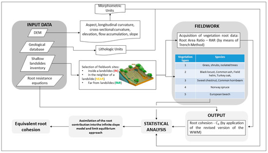
Figure 1.
Flow diagram outlining input data, materials and methods.
2.1. Geological and Vegetational Framework of the Study Area
The study area is located in the Garfagnana Valley in the Northern Apennines (Italy; Figure 2). The area extends for about 240 km2 along the Serchio River Valley, reaching the maximum altitude of about 2000 m a.s.l. The Garfagnana Valley can be described as a tectonic graben located within a series of NW-SE-oriented extensional structures that dissect the contractional structures related to the Apennine orogeny [45,46,47,48]. The high landslide susceptibility in Northern Tuscany can be explained in terms of geological, geomorphological and climatic characteristics [49,50]. Due to the proximity of the Ligurian Sea to the Northern Apennines ridges, this is one of the rainiest areas in the whole Italian peninsula, where the mean annual precipitation ranges from 1500 mm/year to 2300 mm/year [45]. Climatic conditions are directly related to the morphological features present in the study area; indeed, Alpi Apuane exerts a screening action towards humid air flows with a consequent condensation, which results in heavy rainy events [2]. As an example, in the period 2008–2014, 45 intense rainfall events were recorded [50]. About 81% of the study area is covered by forests, which are mainly represented by broadleaf forests with chestnut (Castanea sativa Mill.), beech (Fagus sylvatica L.) and oak (Quercus spp.) trees being the dominant species, and needleleaf forests dominated by Norway spruce (Picea abies (L.) H. Karst.) [6]. The geological, tectonic and geomorphological evolution has made this area particularly interesting for research activities aimed at studying shallow landslide phenomena (Figure 3).
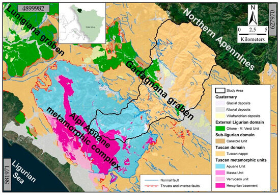
Figure 2.
Tectonic setting of the study area, adapted from “DB Geologico Regionale” [51] (Coordinate system: RDN2008, TM32).
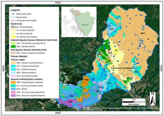
Figure 3.
Location and geology of the study area, adapted from “DB Geologico Regionale” [51] (Coordinate system: RDN2008, TM32).
The geology of the valley includes almost all the tectonic units (Ligurian and Subligurian Units, the Tuscan Nappe and the Tuscan Metamorphic Units) that make up the Northern Apennines (Figure 3) [52]. In the western sector, the valley ridges are usually made up of carbonate rocks with slope gradients greater than 60° (Figure 3). Here, rock usually crops out, with discontinuous vegetation and local scattered forest areas. Moving downslope, metamorphic sandstone and schists prevail, with the bedrock usually covered by talus and scree deposits. Slope steepness is usually moderate (ca. 25–40°), and hillslope deposits mantled by dense forest (mainly chestnut forests) are widespread. The hillslope deposits covering metamorphic sandstone and schists are usually 0.5–2 m thick and are often involved in landsliding. The eastern sector shows more uniform outcropping conditions with the occurrence of the Macigno (MAC) silico-clastic arenaceous flysch (about 45% of the study area; Figure 3), which is composed of thick layers of sandstones with siltstones and subordinate pelitic interbeds [5,45]. In the mid and upper sectors of the valley, layers (1.5–5 m thick) of colluvial deposits overlie the bedrock.
2.2. Input Data
An intensive field survey was carried out to check the available landslide inventory accuracy and to acquire further engineering–geological information about landslides. For the study area, a new multitemporal shallow landslide inventory was obtained by undertaking a visual interpretation of orthophoto maps acquired between 2003 and 2016 [53]. Lithologic data and morphometric parameters (aspect, longitudinal curvature, cross-sectional curvature, elevation, slope and flow accumulation (i.e., contributing area)) were extracted using the available geological map of Tuscany (scale 1:10,000) and the DEM (10 m pixel size) [51]. Indeed, the extraction of landforms was performed by means of unsupervised classification based on the Iterative Self-Organizing Data Analysis (ISODATA) technique [54]. This method is a classification technique that allows us to extract regions of contiguous pixels based on the analysis of a certain number of continuous variables. This technique is often used for the geomorphological classification of landscapes using DEM derivates [54]. ISODATA uses a maximum-likelihood decision rule to calculate class means that are uniformly distributed in the space and then iteratively clusters the remaining pixels using minimum-distance techniques so that clusters are the results of grouping pixels in a multivariate space. Four lithologic classes (Table 1) and five morphometric units (Table 2) were identified in order to evaluate the root data distribution towards lithologic and morphometric features. The above-mentioned features were also analyzed with respect to landslide distribution.

Table 1.
Lithologic classes within the study area (square brackets represent marginal-extent lithologies).
Table 2.
Morphometric units detected in the study area.
2.3. Fieldwork and Outputs
In order to assess the role of vegetation in shallow landslide occurrence, field measurements of root data (root area ratio—RAR) were carried out inside (IN), in the neighbor of (NEAR, within 10 m) and far from (FAR, < ca. 1 km) shallow landslide locations following the strategy adopted by Marzini et al. [6] (Figure 4). Root features were assessed within soil by digging vertical trenches [55]. A total number of 150 measurement sites were identified during the one-year field survey (March 2018–March 2019) (Table 3). In detail, for any visited landslides, characters commonly reported in the literature [56,57] were acquired, such as: involved materials, type of movement [58], depth of hillslope deposits, height of the main scarp, width of the crown and length of the depletion zone. Measurement sites were classified according to their different dominant vegetation types (Table 4).
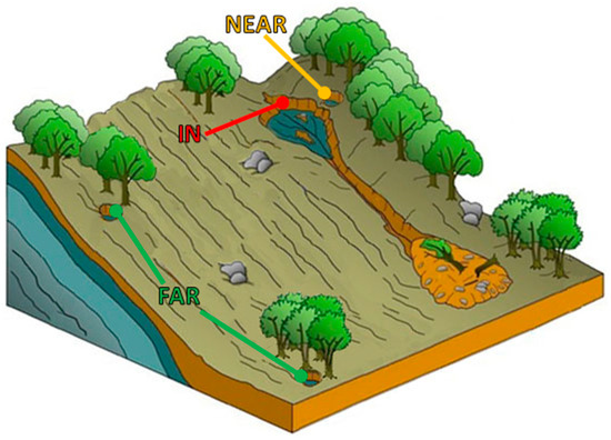
Figure 4.
Acquisition data field strategy adopted during the survey: vegetation data acquired inside (IN), in the neighbor of (NEAR) and far from (FAR; <1 km) shallow landslide locations (from [6]).
Table 3.
Number of measurement sites according to the adopted sampling scheme.
Table 4.
Vegetation types observed in the sampled plots.
The RAR and root strength (Tr) were evaluated in the trenches. RAR data were estimated through the direct application of the trench method [12,18,55,59], with a typical trench width of 0.6–0.8 m and depth of 1–1.5 m (hillslope deposit/bedrock discontinuity depth). In detail, RAR data were acquired through root counting by on-site manual measurements using a digital caliper. Trenches near the landslide main scarps (IN) and at NEAR and FAR measurement sites were dug so that for each measurement three different near-vertical profiles could be obtained: left side, frontal and right side profiles (Figure 5).
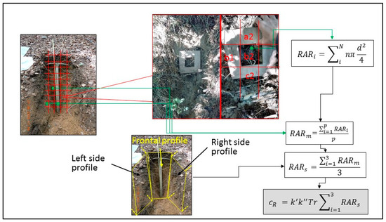
Figure 5.
RAR acquisition field strategy adopted during the survey and method for root cohesion cR estimation (N: number of diameter classes; n: number of analyzed root features; d: diameter class size; p: number of cells within the grid of each profile; RARi: RAR related to each cell; RARm: RAR related to each profile grid; RARs: RAR related to a single measurement site; k′ and k″: additional factors of the revised version of the Wu and Waldron Model; Tr: root strength; b1, a2, b2, c2: examples of grid cells).
Each trench was realized away from the trees’ location, so as to collect RAR data where unfavorable conditions are expected in terms of root reinforcement for slope stability (i.e., where root density is lower). Indeed, it can be assumed that landslide failure surfaces tend to develop where stability factors (i.e., soil cohesion and root reinforcement) are unfavorable. In other words, the field data acquisition strategy allowed us to collect RAR data in the most representative locations for the assessment of stability conditions. A grid of cells of 100 cm2 was overlapped on each profile in order to obtain RAR data (red grid in Figure 5). For each cell, roots were counted and grouped into different diameter classes, then RARi was calculated by using the following formula [12,42,60]:
where “i” is the root diameter class, “n” is number of analyzed root features, “N” indicates the number of diameter classes. For each profile grid, the corresponding RARm was calculated using the following formula:
where “RARi” is related to a single cell and “p” indicates the number of cells within the grid. Finally, the RAR related to a single measurement site (RARs) was determined with the following formula:
where “p” represents the portions of the profile: left side, frontal and right side (Figure 5).
The Wu and Waldron Model (WWM) was applied in order to estimate the additional cohesion cR provided by roots in the soil. This model was proposed several years ago by Wu [22] and Waldron [21] and requires RAR and root strength (Tr) data. It assumes that roots are cylindrical and elastic, they extend perpendicular to the shear surface, and they do not influence the soil friction angle [23,40]. Two additional factors, named k’ and k’’, respectively, were successively implemented in the model’s original version to take into account the root inclination before the enforcement by shear forces and the corresponding deformation, as well as to reduce the root cohesion overestimation [14,61]. Once RARs and root strength were calculated, cR was estimated by the application of the revised version of the WWM:
Regarding the mobilized root strength, two different conditions can be distinguished within a landslide: the main scarp, in which roots undergo tensile and pullout stresses, and lateral scarps, in which roots undergo shear and pullout stresses [28,41,62,63]. Focusing on the main scarp, roots will break or pullout depending on, respectively, their tensile and pullout strength [62,64]. In detail, a single root undergoes either breakage or pullout depending on the magnitude of the peak strength towards either traction or pullout behavior. A root will break if, as strain increases, the tensile peak strength is lower than soil-root friction; a root will slip out if opposite conditions develop. Similar rules apply to roots located in the lateral scarps (Figure 6).
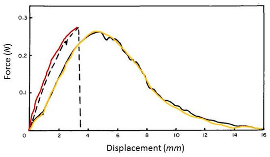
Figure 6.
Force–displacement curves for a broken root (red dashed line) and a pulled-out root (yellow continuous line), adapted from [41].
Root tensile and pullout strength data were obtained through the application of strength–diameter relationships from the literature, commonly associated with a power-law form [28,64]:
where Tr is the root strength for each root diameter class, while a and b are species-dependent parameters (Table 5) and d is the root diameter.
Table 5.
Coefficients a and b related to root tensile and pullout strengths; because of the lack of pullout coefficients for species different from the Norway spruce, we have adopted the Norway spruce coefficients for all the vegetation types.
As every measurement site is characterized by three different profiles (Figure 5), for each measurement site the root cohesion cR (related to both the tensile and pullout root strengths) was determined as defined in the Equation (4). Therefore, the root cohesion cR is based on the average of three independent RAR measurements. Assuming the same RAR and k parameters (see below), cR will correspond to the least value between the tensile or pullout cR (i.e., the strength actually mobilized during shallow landsliding). Regarding k′ and k″, Table 6 and Table 7 report the values commonly adopted in the literature. Both parameters show a wide variability; regarding the first one, despite the common value utilized being equal to 1.2 [21,61], Thomas and Pollen-Bankhead [68] show that the adoption of a unit value is more appropriate to prevent cR overestimation. Therefore, in this work, we have considered two different scenarios to evaluate cR: a conservative scenario (named “a”), in which k′ = 1 and k″ = 0.12, and a non-conservative scenario (named “b”), in which k′ = 1.2 and k″ = 0.5 [69].
Table 6.
Values of k′ adopted in the literature.
Table 7.
Values of k″ adopted in the literature.
Finally, due to the challenging task represented by the integration of root reinforcement into the slope stability models (especially when large areas are considered), a method for the assimilation of the lateral root reinforcement into the infinite slope model and limit equilibrium approach is presented and applied (see Section 4).
2.4. Statistical Analysis
The Chi-square test was applied in order to verify the normal distribution of root vegetation data relative to the three location types: inside (IN), in the neighbor (NEAR) and far (FAR) from shallow-landslide locations; it showed the absence of normal distributions. Significant statistical differences between datasets were determined by the non-parametric Kruskal–Wallis test. For all the tests, the significance level was set to 0.05. Statistical analyses were performed using Origin 2018 (Origin Lab Corporation, Northampton, MA, USA, 2018) and Real Statistics Resource Pack software (Release 5.4).
3. Results
Table 8 reports the shallow landslide frequency distribution for the study area with respect to lithologic classes, morphometric units and vegetation types. The results highlight that shallow landslides are more frequent in the lithologic class L1, including arenaceous and meta-arenaceous flysch, which correspond to the most widespread lithologies in the study area (45%). These considerations can also be extended to the morphometric unit E (upper portion of slopes and valleys), representing 37% of the study area. Finally, vegetation type 3 (including sweet chestnut and common hornbeam) includes the largest number of shallow landslides, depending on the fact that the Castanetum zone, which develops up to 900 m a.s.l., covers most of the study area.
Table 8.
Shallow-landslide frequency distribution for the study area. For a total number of 40 shallow landslides (IN sites), the absolute frequencies (Abs. freq.) related to lithologic classes, morphometric units and vegetation types are listed. For the meaning of lithologic classes, morphometric units and vegetation types, see Table 1, Table 2 and Table 4, respectively.
As for the results of RAR measurement, we could collect these data for 129 sites over the total number of sites (150) under analysis. Figure 7 shows the values of RAR distribution within the three different location types: IN, NEAR and FAR. The application of the Kruskal–Wallis test highlights that NEAR data are statistically separated from IN and FAR data populations (p-values of 0.006 and 0.004, respectively). In detail, the NEAR population shows a median value equal to 1.44, whereas the IN and FAR data populations show median values equal to 0.77 and 0.89, respectively.
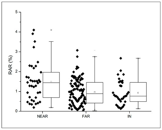
Figure 7.
Boxplots of RAR data in the three main data-acquisition location types. The box represents data within the first and the third quartile, the square symbol represents the mean value, × symbol represents the outlier, and lines extending parallel from the box are the whiskers in the 10–90 range.
The application of the Kruskal–Wallis test shows that, when considering lithologic classes and morphometric units, RAR data statistically belong to a single population (Figure 8 and Figure 9), whereas, when focusing on vegetation types, RAR data show the distribution reported in Figure 10. In detail, lithologic classes L1 (arenaceous and meta-arenaceous flysch), L2 (limestone, calcareous flysch, dolostone, marble), L3 (marl, claystone, siltstone, basalt and ultramaphites) and L4 (lacustrine shale, sandy shale, terraced alluvial deposits) show median values of 0.90, 0.50, 0.86 and 1.28, respectively (Figure 8). Based on these results, it can be stated that geology exhibits a limited control on root density distribution. The same considerations hold for the morphometric analysis. Indeed, morphometric units A (gentle ridges and alluvial areas (<200 m a. s. l.)), B (steep ridges (>600 m a. s. l.)), C (gentle slopes and gentle ridges (200–600 m a. s. l.), D (flat to convex slopes) and E (upper portion of slopes) show median values equal to 0.73, 0.44, 1.28, 0.88, and 0.76, respectively (Figure 9). Based on these results, it can be stated that even morphology exhibits a limited control on root density distribution. The apparent lack of lithologic and morphometric influence on vegetation data may be an effect of the spatial sampling strategy adopted, this latter being not based on catchment scale acquisition criteria. The same considerations can be drawn for the vegetation types. Indeed, focusing on the vegetation types, the Kruskal–Wallis test highlights that type 1 (characterized by grass, shrubs and isolated trees), is separated from the other types. In detail, vegetation type 1, type 2 (Black locust, Common ash, Field helm, Turkey oak), type 3 (Sweet chestnut, Common hornbeam), type 4 (Norway spruce) and type 5 (European beech) show median values equal to 0.14, 1.06, 1.23, 0.85 and 0.86, respectively (Figure 10).
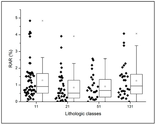
Figure 8.
Boxplots of RAR data for the four lithological classes considered. The box represents data within the first and the third quartile, the square symbol represents the mean value, × symbol represents the outlier, and lines extending parallel from the box are the whiskers in the 10–90 range. For the meaning of lithologic classes, see Table 1.
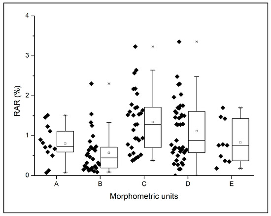
Figure 9.
Boxplots of RAR data for the five morphological classes considered. The box represents data within the first and the third quartile, the square symbol represents the mean value, × symbol represents the outlier, and lines extending parallel from the box are the whiskers in the 10–90 range. For the meaning of morphometric units, see Table 2.
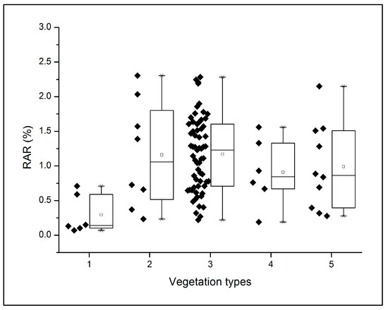
Figure 10.
Boxplots of RAR data for the five vegetation types considered. The box represents data within the first and the third quartile, the square symbol represents the mean value, × symbol represents the outlier, and lines extending parallel from the box are the whiskers in the 10–90 range. For the meaning of vegetation types, see Table 4.
RAR data were also analyzed as a function of measurement depth. Indeed, the development of vegetation (including roots) is strongly influenced by ecological, geological, genetic and climatic factors [23,33]; generally, root density decreases as the depth increases and this is due to changes in nutrients and moisture availability [12]. In agreement with the literature [78], in this study, a RAR reduction with depth was observed, as shown in Figure 11. Namely, the RAR tends toward nil values when approaching to depth of ca. 0.70–0.80 m. This behavior does not show any correlation with the spatial distribution of shallow landslides (IN, NEAR and FAR curves in Figure 11).
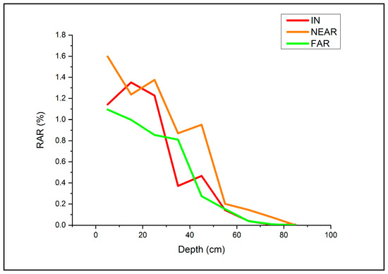
Figure 11.
Variation of the RAR with depth for the different location types (“FAR”—green line, “NEAR”—orange line and “IN”—red line).
4. Assimilating the Contribution of Root Reinforcement into the Infinite Slope Model and Limit Equilibrium Approach
Focusing on shallow landslides, the infinite slope model and limit equilibrium approach assume the basal-failure plane (fpSD-S) to be parallel to the ground surface and close to the hillslope deposits/substratum contact (SD-S) (Figure 12).
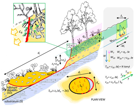
Figure 12.
Effects of vegetation on shallow slope stability and scheme of acting/reacting forces for the infinite slope model and limit equilibrium approach (water effects are neglected in order to simplify the representation). Heavenly color: substratum (S); yellow: hillslope deposits (SD); orange: landslide mass body. Symbols: dl: landslide length, dw: landslide scarp width, fpSD-S: hillslope deposits/substratum contact (basal-failure plane for the infinite slope model), zS: substratum depth, zSD: hillslope deposits depth, zR: roots maximum depth, Δx: width of the slope element potentially unstable representative of the hillslope deposits, Δdl: projection of Δx on fpSD-S, SB: landslide basal area, SLR: landslide root lateral area, qV: vegetation load (assumed uniformly distributed), γ: hillslope deposits unit weight, cR: root cohesion, ceR: equivalent root cohesion, cSD: hillslope deposits cohesion, ϕ: hillslope deposits friction angle. Symbols related to the forces acting at the base of the slope element: W: total weight, WV: vegetation weight, WSD: hillslope deposits weight, FN: component of W normal to fpSD-S, FT: component of W parallel to fpSD-S (destabilizing shear stress), T: total shear strength, TR: root shear strength (stabilizing lateral root reinforcement), TSD: hillslope deposits shear strength (stabilizing). Adapted from [79].
Moreover, the balance between shear stress (FT) and shear strength (T) is evaluated along the fpSD-S. Therefore, the strength mobilized along the landslide flanks, where root reinforcement develops, is neglected. Zhou et al. [80] found that different hillslope configurations related to the lateral root reinforcement. In detail, three different scenarios related to the root extraction dynamics were described: (1) roots anchored in the sliding mass across a tension crack, (2) roots originating from the stable mass, and (3) roots originating from the stable mass with multiple block failures [81]. Our scheme reported in Figure 12 refers to the combination of the first and second scenario, with roots occurring within both the stable and sliding masses.
Lateral root reinforcement represents a key factor in shallow landslide development [82]. Indeed, crucially, roots do not reach the depth of the shallow landslide basal failure plane (usually 1–2 m) [82]. In Figure 13, the morphometric characters (basal failure plane depth, landslide length and landslide scarp width) of the shallow landslides visited are reported. The basal-failure plane depth shows a median value of ca. 0.8 m, so, considering the root density decrease with depth (Figure 11), roots within the mobilized landslide volume do not crucially provide significant reinforcement along the basal-failure plane. On the contrary, those roots occurring within both the landslide scarp and flanks clearly contribute to shear strength.
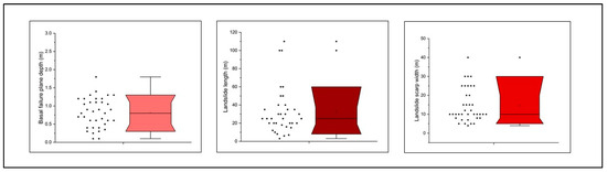
Figure 13.
Boxplots of shallow landslide basal failure plane (left, pink boxplot), length (center, dark red boxplot) and scarp width (right, red boxplot) for the shallow landslides visited during fieldwork. The boxes represent data within the first and third quartiles, the square symbols represent the mean value, and lines extending parallel from the box are the whiskers in the 10–90 range.
Furthermore, 2D infinite slope stability models assume that root cohesion influences stability along the base of the slide mass only, despite lateral root reinforcement controlling shallow landslide initiation [1,83]. Therefore, the contribution of the roots located within both the scarp and flanks must be introduced within these models as an equivalent root cohesion ceR, which is assumed to be mobilized along the landslide basal failure plane. In detail, the lateral root reinforcement TR is assumed to develop to the depth zR on the landslide scarp and flanks (extent SLR); hence:
Therefore, a contribution equivalent to TR is assumed to be mobilized at the basal failure plane fpSD-S (extent SB), so that:
where ceR is the equivalent root cohesion, corresponding to (Figure 12):
Figure 14 shows the distribution of ceR obtained by considering, for each of the 40 visited landslides (Table 3), the local values of SB, SLR, root maximum depth zR, landslide length dl and landslide scarp width dw. These values are obtained for two k′ and k″ scenarios (k′a = 1 and k′b = 1.2; k″a = 0.12 and k″b = 0.5) [68]. For the conservative scenario (a), the mean ceR is ca. 2 kPa, whereas ceR ≅ 3 kPa is obtained for the non-conservative scenario (b). In addition, the third quartile of the two ceR distributions are ca. 4 kPa and 10 kPa, respectively.
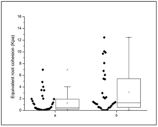
Figure 14.
Boxplots of the equivalent root cohesion ceR values estimated considering a conservative scenario (a) and a non-conservative scenario (b). The boxes represent data within the first and the third quartile, the square symbols represent the mean value, × symbol represents the outlier, and lines extending parallel from the box are the whiskers in the 10–90 range.
5. Discussion
The results of this research show that root reinforcement plays a relevant role in the development of shallow landslides. Indeed, the analysis of the root vegetation data showed a RAR differentiation according to the class of measurement sites (inside a shallow landslide—IN, in the neighbor of a shallow landslide—NEAR, far from shallow landslides—FAR). Particularly, the stability of slopes for the FAR sites can be considered the result of the combined action of different predisposing factors (lithology, soil geotechnical properties, slope, elevation, land use, climatic conditions, etc.), including vegetation [84,85]. Instead, the identification of higher RAR values at NEAR sites compared to IN site values allows us to state that vegetation, at least RAR features, exerts a control action on shallow landslide development, assuming that typical predisposing factor conditions can occur in the landslide areas and are reasonably constant in the neighbor of shallow landslides.
Therefore, this approach allowed us to make a new RAR dataset available describing the spatial variability of root systems for the Garfagnana study area. The analysis of this dataset highlights the role of root systems in shallow landslides, in agreement with Roering et al. [17] and Moos et al. [86]. These authors provided results concerning the characteristics of roots close to landslide scarps and the clear link between landslide susceptibility and root reinforcement. In detail, in the work by Roering et al. [17], the tree position, along with the characteristics of trees, represented an important factor in the study of the spatial variability of root strength, as well as shallow landslides occurring within forests. Indeed, root reinforcement could be predicted by mapping the presence of trees on potentially unstable slopes, suggesting that vegetation distribution plays an important role. Moos et al. [86] found that the occurrence of landslides was higher in zones with low root reinforcement (which correspond to IN locations in our study). From the perspective of the local-scale spatial variability of root reinforcement, some similarities with our approach can be found in the work of Hales et al. [87], where the influence of the positions on both the distribution and root reinforcement in an instability-phenomena-prone landscape was studied. According to their results, topographic position significantly affected the root reinforcement, as nose locations showed significantly higher values than hollows. These results agree, in turn, with the work of Dietrich et al. [88], which states that landslides most commonly occur in flow accumulation zones. Moreover, our results agree with the findings of Marzini et al. [6], in which differences in terms of lignin and cellulose proportions (structural chemical components that provide root mechanical properties) were found moving from landslides (i.e., IN sites) to stable locations (decrease in the lignin/cellulose ratio moving from landslides to stable areas).
RAR values, as obtained by the implementation of the trench method, resulted in the order of 5% or lower, and they are coherent with values known from the literature for similar environmental conditions [23,32,61]. Regarding the depth reached by roots, results are smaller compared to the literature [78,89,90] and show maximum RAR values at a depth of 0.20–0.50 m, in agreement with Li et al. [24]. This evidence represents the result of the combined action of nutrient decrease, aeration, water availability and layer compaction. Smaller depths may be explained by the acquisition data strategy adopted during the field survey: the trench method was applied not close to trees so as to collect RAR data in locations unfavorable for root reinforcement (i.e., lower root density and resulting worse stability conditions in terms of additional cohesion). Indeed, according to the fact that landslide failure planes tend to develop following weakness zones (i.e., poor geotechnical properties of the hillslope deposit), RAR data collected near trees are not representative, because the failure plane will barely develop where root reinforcement is greater.
Many studies have highlighted the role of the roots in hillslope stability considering only basal root reinforcement [1,19]. To the best of our knowledge, the geometrical representation of a shallow landslide has led to a distinction between basal root reinforcement and lateral root reinforcement [82]. The former acts on the basal shear surface of the landslide and would be the most effective reinforcement mechanism if uniformly distributed along with the profile [64]. However, generally, roots do not reach the shallow landslide basal failure plane depth (usually 1–2 m) and, as depicted from our root density data, the progressive RAR reduction with depth affects the role of root reinforcement. Namely, our findings show that roots within the mobilized landslide volume cannot contribute to the basal reinforcement of shallow landsliding. Moreover, some studies highlighted that lateral root reinforcement may be activated along the potential landslide flanks, also influencing their size [1]. In fact, the stabilizing role exercised by lateral roots was shown to be important for landslides with areas up to 1000 m2 [82], where roots do not cross the basal failure plane. Therefore, this literature framework, along with our field observations, make the proposed method for the implementation of the lateral root reinforcement into the infinite slope model and limit equilibrium approach, by introducing the equivalent root cohesion parameter (ceR)—a relevant outcome of this research. The ceR values estimated for two scenarios corresponding to different values of k′ and k″ (Table 6 and Table 7) were satisfactory and reliable (mean of ca. 2–3 kPa and third quartile equal to ca. 4 kPa and 10 kPa for conservative and non-conservative scenarios, respectively (Figure 14)). Indeed, these values are in general agreement with the Schwarz et al. [82] findings about the Vinchiana landslide case study (Tuscany, Italy). Results from these authors are based on the implementation of lateral root reinforcement into the fiber bundle model [35] and indicate the mobilization of a root reinforcement contribution always lower than 20 kPa along the landslide scarp. Nevertheless, based on our findings, the implementation and calibration of the k additional factors into the WWM model represent both a fundamental and critical step in the root reinforcement estimation for landslide stability analysis and, therefore, caution must be taken in the selection of these numerical values [19,23].
An issue to be considered when analyzing the results of our research is represented by the spatio-temporal heterogeneity of forest stand properties. Our approach is based on root reinforcement parameters obtained from an intensive and spatially distributed field survey carried out within almost one year. The temporal variation of root reinforcement may depend on two types of processes: one is the seasonal dynamics of root distribution and mechanical properties, and the second is the long-term dynamics of both tree and stand [35]. Moreover, the post-disturbance relationships between root reinforcement recovery dynamics in a forest stand and the shallow landslide susceptibility change must also be taken into account. Post-disturbance shallow landslide susceptibility mainly depends on the root decay of the dying trees, the recovery rate of the new stand in terms of roots and canopy cover, and the frequency and magnitude of rainfall events (e.g., [91]). In this spatio-temporal complex framework, the epoch of occurrence of a landslide, as well as the epoch of fieldwork survey, represent important conditions that may influence the accurate evaluation of root reinforcement at both seasonal and long-term scales. In principle, a survey should be performed immediately after the landslide event. In practice, this is a tricky task, as landslide inventories are generally obtained by either the interpretation or classification of remote sensing imagery [45] with a temporal resolution of several years; hence, they seldom provide the landslide activation epoch. Moreover, the inventories do not generally undergo real-time updating. The inventory we used in this research is a multitemporal inventory obtained by interpretation of 2003–2016 orthophotos with a temporal resolution of ca. 2–3 years. Therefore, our data may be affected by seasonal uncertainties as well as long-term effects related to a time span of less than 15 years. Nevertheless, the results show a correlation between root reinforcement and landslide distribution, suggesting that the effect of the above issues does not obliterate the main signal of the analyzed processes. The results are relevant for spatial landslide-susceptibility assessment [91].
The landslide frequency distribution analysis with respect to lithologic classes is consistent with D’Addario et al. [92], who analyzed the same distribution for Southern Lunigiana (Tuscany, Italy; Figure 2). Several physical and chemical properties of bedrock, as well as morphometric features, can play a role in the distribution of vegetation [93,94]. Despite this, our RAR results show no relevant differences following both lithologic classes and morphometric units. Our results are in contrast with the Tron et al. findings [90]. Indeed, according to the literature, pedology, rainfall distribution and plant stand age are more important than the species [90,95]. In detail, referring to the work of Laio et al. [96], the shape of the root distribution along a portion of a generic trench is mainly determined by the distribution of the rainfall. Moreover, root systems are deeper where the soils are coarse-textured and the evaporative demand slightly exceeds precipitation. Roots grow only as deeply as needed to fulfil plant needs [96]. The apparent lack of lithologic and morphometric influence on vegetation data may be an effect of the spatial sampling strategy adopted, with the latter not being based on catchment scale acquisition criteria. Regarding vegetation types, RAR data show the separation of type 1 (including grass, shrubs and isolated trees) from the other types. Type 1 values are higher than values related to herbaceous and shrub Mediterranean species [36,61]. This outcome may be explained by the occurrence of isolated trees (characterized by a more complex root system compared to grass and shrubs) in this category.
6. Conclusions
This work provides new insight into the correlation between root reinforcement and shallow landslides. Namely, differences in terms of root density (expressed by the RAR) moving from shallow landslides to neighboring areas were observed. Therefore, the RAR obtained in the field by implementing the trench method may be considered a relevant parameter for the evaluation of the vegetation contribution to shear strength in slope stability analyses.
RAR data allowed us to estimate root cohesion cR value intervals by means of the revised version of the WWM model, with the aim of quantifying the role of root reinforcement in the infinite slope model and limit equilibrium approach.
The analysis of root distribution with depth allowed us to observe that roots generally cannot reach the depth of shallow landslide basal failure plane. Therefore, we proposed and applied a new method for the implementation of lateral root reinforcement in the infinite slope model and limit equilibrium approach. The method introduces a parameter named equivalent root cohesion ceR, conveying information on both lateral root depth and extension to the shallow landslide basal surface. The method represents a quantitative achievement for the evaluation of roots’ contribution to physically based slope stability models for shallow landslides.
Further insights will be dedicated to the refinement of the field methodology, as well as to the integration of field data within fiber bundle models available in the literature. Moreover, new data concerning the ecological successions established in shallow landslides could be acquired.
Author Contributions
Conceptualization, L.D. and L.M.; methodology, L.D., L.M., E.D. and F.C.; software, L.M. and F.C.; validation, L.M., M.P.P. and E.D.; formal analysis, L.M.; investigation, L.M., M.P.P., E.D. and L.D.; resources, L.D.; data curation, L.M.; writing—original draft preparation, L.M.; writing—review and editing, L.D., L.M., E.D., M.P.P. and F.C.; visualization, equal contribution of all authors; supervision, L.D.; project administration, L.D.; funding acquisition, L.D. All authors have read and agreed to the published version of the manuscript.
Funding
This research was funded by Università di Siena—Dipartimento di Scienze Fisiche, della Terra e dell’Ambiente within the projects: “Accordo di collaborazione scientifica cofinanziato da Consorzio LaMMA e Università di Siena” (Project leader: L.D.), under grant agreement n. B53C22005240002.
Data Availability Statement
All data generated or analyzed for this study are included in this article, and the related datasets are available from the corresponding author on reasonable request.
Conflicts of Interest
The authors declare no conflict of interest.
References
- Murgia, I.; Giadrossich, F.; Mao, Z.; Cohen, D.; Capra, G.F.; Schwarz, M. Modeling shallow landslides and root reinforcement: A review. Ecol. Eng. 2022, 181, 106671. [Google Scholar] [CrossRef]
- Giannecchini, R.; Galanti, Y.; D’Amato Avanzi, G. Critical rainfall thresholds for triggering shallow landslides in the Serchio River Valley (Tuscany, Italy). Nat. Hazards Earth Syst. Sci. 2012, 12, 829–842. [Google Scholar] [CrossRef]
- Meisina, C.; Scarabelli, S. A comparative analysis of terrain stability models for predicting shallow landslides in colluvial soils. Geomorphology 2007, 87, 207–223. [Google Scholar] [CrossRef]
- Persichillo, M.G.; Bordoni, M.; Meisina, C.; Bartelletti, C.; Barsanti, M.; Giannecchini, R.; D’Amato Avanzi, G.; Galanti, Y.; Cevasco, A.; Brandolini, P.; et al. Shallow landslides susceptibility assessment in different environments. Geomat. Nat. Hazards Risk 2017, 8, 748–771. [Google Scholar] [CrossRef]
- Tofani, V.; Bicocchi, G.; Rossi, G.; Segoni, S.; D’Ambrosio, M.; Casagli, N.; Catani, F. Soil characterization for shallow landslides modeling: A case study in the Northern Apennines (Central Italy). Landslides 2017, 14, 755–770. [Google Scholar] [CrossRef]
- Marzini, L.; Ciofini, D.; Agresti, J.; Ciaccheri, L.; D’Addario, E.; Disperati, L.; Siano, S.; Osticioli, I. Exploring the Potential of Portable Spectroscopic Techniques for the Biochemical Characterization of Roots in Shallow Landslides. Forests 2023, 14, 825. [Google Scholar] [CrossRef]
- IPCC. Contribution of Working Groups I, II and III to the Assessment Report 6 of the Intergovernmental Panel on Climate Change; 2022: Synthesis Report; IPCC: Geneva, Switzerland, 2022. [Google Scholar]
- Amaddii, M.; Rosatti, G.; Zugliani, D.; Marzini, L.; Disperati, L. Back-Analysis of the Abbadia San Salvatore (Mt. Amiata, Italy) Debris Flow of 27–28 July 2019: An Integrated Multidisciplinary Approach to a Challenging Case Study. Geosciences 2022, 12, 385. [Google Scholar] [CrossRef]
- Masi, E.B.; Tofani, V.; Rossi, G.; Cuomo, S.; Wu, W.; Salciarini, D.; Caporali, E.; Catani, F. Effects of roots cohesion on regional distributed slope stability modelling. Catena 2023, 222, 106853. [Google Scholar] [CrossRef]
- Corominas, J.; van Westen, C.; Frattini, P.; Cascini, L.; Malet, J.P.; Fotopoulou, S.; Catani, F.; van den Eeckhaut, M.; Mavrouli, O.; Agliardi, F.; et al. Recommendations for the quantitative analysis of landslide risk. Bull. Eng. Geol. Environ. 2014, 73, 209–263. [Google Scholar] [CrossRef]
- Skempton, A.W.; Delory, F.A. Stability of natural slopes in London clay. In Selected Papers on Soil Mechanics; Thomas Telford Publishing: London, UK, 1957; pp. 378–381. [Google Scholar] [CrossRef]
- Bischetti, G.B.; Chiaradia, E.A.; Simonato, T.; Spaziali, B.; Vitali, B.; Vullo, P.; Zocco, A. Root strength and root area ratio of forest species in Lombardy (Northern Italy). Plant Soil 2005, 278, 11–22. [Google Scholar] [CrossRef]
- Pisano, M.; Cardile, G. Probabilistic Analyses of Root-Reinforced Slopes Using Monte Carlo Simulation. Geosciences 2023, 13, 75. [Google Scholar] [CrossRef]
- Giadrossich, F.; Schwarz, M.; Cohen, D.; Cislaghi, A.; Vergani, C.; Hubble, T.; Phillips, C.; Stokes, A. Methods to measure the mechanical behavior of tree roots: A review. Ecol. Eng. 2017, 109, 256–271. [Google Scholar] [CrossRef]
- Greenwood, J.R.; Norris, J.E.; Wint, J. Assessing the contribution of vegetation to slope stability. Proc. Inst. Civ. Eng.-Geotech. Eng. 2004, 157, 199–207. [Google Scholar] [CrossRef]
- Kokutse, N.K.; Temgoua AG, T.; Kavazović, Z. Slope stability and vegetation: Conceptual and numerical investigation of mechanical effects. Ecol. Eng. 2016, 86, 146–153. [Google Scholar] [CrossRef]
- Roering, J.J.; Schmidt, K.M.; Stock, J.D.; Dietrich, W.E.; Montgomery, D.R. Shallow landsliding, root reinforcement, and the spatial distribution of trees in the Oregon Coast Range. Canadian Geotech. J. 2003, 40, 237–253. [Google Scholar] [CrossRef]
- Tosi, M. Root tensile strength relationships and their slope stability implications of three shrub species in the Northern Apennines (Italy). Geomorphology 2007, 87, 268–283. [Google Scholar] [CrossRef]
- Masi, E.B.; Segoni, S.; Tofani, V. Root Reinforcement in Slope Stability Models: A Review. Geosciences 2021, 11, 212. [Google Scholar] [CrossRef]
- Schwarz, M.; Rist, A.; Cohen, D.; Giadrossich, F.; Egorov, P.; Büttner, D.; Stolz, M.; Thormann, J.J. Root reinforcement of soils under compression. J. Geophys. Res. Earth Surf. 2015, 120, 2103–2120. [Google Scholar] [CrossRef]
- Waldron, L.J.; Dakessian, S. Soil reinforcement by roots: Calculation of increased soil shear resistance from root properties. Soil Sci. 1981, 132, 427–435. [Google Scholar] [CrossRef]
- Wu, T.H.; McKinnell, W.P., III; Swanston, D.N. Strength of tree roots and landslides on Prince of Wales Island, Alaska. Can. Geotech. J. 1979, 16, 19–33. [Google Scholar] [CrossRef]
- Bischetti, G.B.; Chiaradia, E.A.; Epis, T.; Morlotti, E. Root cohesion of forest species in the Italian Alps. Plant Soil 2009, 324, 71–89. [Google Scholar] [CrossRef]
- Li, Y.; Wang, Y.; Ma, C.; Zhang, H.; Wang, Y.; Song, S.; Zhu, J. Influence of the spatial layout of plant roots on slope stability. Ecol. Eng. 2016, 91, 477–486. [Google Scholar] [CrossRef]
- Ni, J.J.; Leung, A.K.; Ng CW, W.; Shao, W. Modelling hydro-mechanical reinforcements of plants to slope stability. Comput. Geotech. 2018, 95, 99–109. [Google Scholar] [CrossRef]
- Reubens, B.; Poesen, J.; Danjon, F.; Geudens, G.; Muis, B. The role of fine and coarse roots in shallow slope stability and soil erosion control with a focus on root system architecture: A review. Trees 2007, 21, 385–402. [Google Scholar] [CrossRef]
- Simon, A.; Collison AJ, C. Quantifying the mechanical and hydrologic effects of riparian vegetation on streambank stability. Earth Surf. Process. Landf. 2002, 27, 527–546. [Google Scholar] [CrossRef]
- Vergani, C.; Chiaradia, E.A.; Bischetti, G.B. Variability in the tensile resistance of roots in Alpine forest tree species. Ecol. Eng. 2012, 46, 43–56. [Google Scholar] [CrossRef]
- Wilkinson, P.L.; Anderson, M.G.; Lloyd, D.M. An integrated hydrological model for rain-induced landslide prediction. Earth Surf. Process. Landf. 2002, 27, 1285–1297. [Google Scholar] [CrossRef]
- Iverson, R.M. Landslide triggering by rain infiltration. Water Resour. Res. 2000, 36, 1897–1910. [Google Scholar] [CrossRef]
- Sidle, R.C.; Ziegler, A.D. The canopy interception-landslide initiation conundrum: Insight from a tropical secondary forest in northern Thailand. Hydrol. Earth Syst. Sci. 2017, 21, 651–667. [Google Scholar] [CrossRef]
- Stokes, A.; Norris, J.E.; van Beek, L.P.H.; Bogaard, T.; Cammeraat, E.; Mickovski, S.B.; Jenner, A.; Di Iorio, A.; Fourcaud, T. How Vegetation Reinforces Soil on Slopes. In Slope Stability and Erosion Control: Ecotechnological Solutions; Norris, J.E., Stokes, A., Mickovski, S.B., Cammeraat, E., van Beek, R., Nicoli, B.C., Achim, A., et al., Eds.; Springer: Dordrecht, The Netherlands, 2008. [Google Scholar] [CrossRef]
- Preti, F. Forest protection and protection forest: Tree root degradation over hydrological shallow landslides triggering. Ecol. Eng. 2013, 61, 633–645. [Google Scholar] [CrossRef]
- Chirico, G.B.; Dani, A.; Preti, F. Coupling Root Reinforcement and Subsurface Flow Modeling in Shallow Landslides Triggering Assessment. In Landslide Science and Practice; Margottini, C., Canuti, P., Sassa, K., Eds.; Springer: Berlin/Heidelberg, Germany, 2013. [Google Scholar] [CrossRef]
- Ngo, H.M.; van Zadelhoff, F.B.; Gasparini, I.; Plaschy, J.; Flepp, G.; Dorren, L.; Phillips, C.; Giadrossich, F.; Schwarz, M. Analysis of Poplar’s (Populus nigra ita.) Root Systems for Quantifying Bio-Engineering Measures in New Zealand Pastoral Hill Country. Forests 2023, 14, 1240. [Google Scholar] [CrossRef]
- Gasser, E.; Perona, P.; Dorren, L.; Phillips, C.; Hübl, J.; Schwarz, M. A New Framework to Model Hydraulic Bank Erosion Considering the Effects of Roots. Water 2020, 12, 893. [Google Scholar] [CrossRef]
- Abernethy, B.; Rutherfurd, I.D. The distribution and strength of riparian tree roots in relation to riverbank reinforcement. Hydrol. Process. 2001, 15, 63–79. [Google Scholar] [CrossRef]
- De Baets, S.; Poesen, J.; Reubens, B.; Wemans, K.; de Baerdemaekers, J.; Muys, B. Root tensile strength and root distribution of typical Mediterranean plant species and their contribution to soil shear strength. Plant Soil 2008, 305, 207–226. [Google Scholar] [CrossRef]
- Coppin, N.J.; Richards, I.G. Use of Vegetation in Civil Engineering; Butterworth-Heinemann: Oxford, UK, 1990. [Google Scholar]
- Danjon, F.; Barker, D.H.; Drexhage, M.; Stokes, A. Using three-dimensional Plant Root Architecture in Models of Shallow-slope Stability. Ann. Bot. 2008, 101, 1281–1293. [Google Scholar] [CrossRef] [PubMed]
- Ennos, A.R. The anchorage of leek seedlings: The effect of root length and soil strength. Ann. Bot. 1990, 65, 409–416. [Google Scholar] [CrossRef]
- Gonzalez-Oullari, A.; Mickovski, S.B. Hydrological effect of vegetation against rainfall-induced landslides. J. Hydrol. 2017, 549, 374–387. [Google Scholar] [CrossRef]
- Zimmermann, A.; Zimmermann, B. Requirements for throughfall monitoring: The roles of temporal scale and canopy complexity. Agric. For. Meteorol. 2014, 189–190, 125–139. [Google Scholar] [CrossRef]
- Luo, Z.; Niu, J.; Xie, B.; Zhang, L.; Chen, X.; Berndtsson, R.; Du, J.; Ao, J.; Yang, L.; Zhu, S. Influence of Root Distribution on Preferential Flow in Deciduous and Coniferous Forest Soils. Forests 2019, 10, 986. [Google Scholar] [CrossRef]
- D’Addario, E. A New Approach to Assess the Susceptibility to Shallow Landslides at Regional Scale as Influenced by Bedrock Geo-Mechanical Properties. Ph.D. Thesis, University of Siena, Siena, Italy, 2021. [Google Scholar]
- Boschetti, T.; Toscani, L.; Barbieri, M.; Mucchino, C.; Marino, T. Low entalphy Na-chlorine waters from the Lunigiana and Garfagnana grabens: Northern Apenninnes, Italy: Tracing fluid connections and basement interaction via chemical and isotopic composition. J. Volcanol. Geotherm. Res. 2017, 348, 12–25. [Google Scholar] [CrossRef]
- Di Naccio, D.; Boncio, P.; Brozzetti, F.; Pazzaglia, F.J.; Lavecchia, G. Morphotectonic analysis of the Lunigiana and Garfagnana grabens (northern Apennines, Italy): Implication for active normal faulting. Geomorphology 2013, 201, 293–311. [Google Scholar] [CrossRef]
- Eva, E.; Solarino, S.; Boncio, P. HypoDD relocated seismicity in northern Apennines (Italy) preceding the 2013 seismic unrest: Seismotectonic implications for the Lunigiana-Garfagnana area. Boll. Geofis. Teor. Appl. 2014, 55, 739–754. [Google Scholar] [CrossRef]
- Maracchi, G.; Genesio, L.; Magno, R.; Ferrari, R.; Crisci, A.; Bottai, L. I Diagrammi del Clima in Toscana; Stampa: Florence, Italy, 2005. [Google Scholar]
- Lavorini, G.; Villoresi, C.; Bottai, L.; Perna, M.; Manetti, F.; Capecchi, V.; Betti, G.; Bartolini, G.; Crisci, A.; Corongiu, M. Analisi dei dissesti associati ad alcuni fenomeni di precipitazione intensa in Toscana attraverso l’analisi di immagini satellitari multi-spettrali. Il Geol. 2015, n.98. [Google Scholar]
- Regione Toscana–DB Geologico. Available online: http://www502.regione.toscana.it/geoscopio/geologia.html (accessed on 10 August 2023).
- Puccinelli, A.; D’Amato Avanzi, G.; Perilli, N. Note illustrative della carta geologica d’Italia alla scala 1:50.000. In Foglio 250 Castelnuovo di Garfagnana; The University of Pisa: Pisa, Italy, 2014. [Google Scholar]
- Regione Toscana-Fototeca. Available online: https://www502.regione.toscana.it/geoscopio/fototeca.html (accessed on 10 August 2023).
- Tou, J.T.; Gonzalez, R.C. Pattern Recognition Principles; Addison-Wesley Publishing: Boston MA, USA, 1974. [Google Scholar]
- Böhm, W. Methods of Studying Root System; Springer: Berlin/Heidelberg, Germany, 1979. [Google Scholar] [CrossRef]
- Amanti, M.; Bertolini, G.; Ceccone, G.; Chiessi, V.; de Nardo, M.T.; Ercolani, L.; Gasparo, F.; Guzzetti, F.; Landrini, C.; Martini, M.G.; et al. Scheda di Censimento dei Fenomeni Franosi Versione 2.33. In Guida al Censimento dei Fenomeni Franosi ed Alla Loro Archiviazione; Miscellanea VI; Servizio Geologico d’Italia: Rome, Italy, 1998. [Google Scholar]
- Pergalani, F.; Padovan, N.; Agostoni, A.; Belloni, A.; Costantini, R.; Crosta, G.; de Andrea, S.; Laffi, R.; Luzi, L.; Sterlacchini, S. Valutazione della Stabilità dei Versanti in Condizioni Statiche e Dinamiche Nella Zona Campione Dell’oltrepo Pavese; Regione Lombardia Settore Tutela Ambientale Servizio Geologico e Tutela delle Acque e Consiglio Nazionale Ricerche; Istituto di Ricerca sul Rischio Sismico: Milano, Italy, 1998; p. 80. [Google Scholar]
- Hungr, O.; Leroueil, S.; Picarelli, L. The Varnes classification of landslide types, an update. Landslides 2014, 11, 167–194. [Google Scholar] [CrossRef]
- Giambastiani, A.; Errico, F.; Preti, E.; Guastini, G. Censini Indirect root distribution characterization using electrical resistivity tomography in different soil conditions. Urban For. Urban Green. 2021, 67, 127442. [Google Scholar] [CrossRef]
- Lateh, H.; Avani, N.; Bibalani, G.H. Investigation of root distribution and tensile strength of Acacia mangium Willd (Fabaceae) in the rainforest. Greener J. Biol. Sci. 2014, 4, 45–52. [Google Scholar] [CrossRef]
- Preti, F.; Giadrossich, F. Root reinforcement and slope bioengineering stabilization by Spanish broom (Spartium junceum L.). Hydrol. Earth Syst. Sci. 2009, 13, 1713–1726. [Google Scholar] [CrossRef]
- Dias, A.S.; Pirone, M.; Urciuoli, G. Review of the Methods for Evaluation of Root Reinforcement in Shallow Landslides. In Advancing Culture of Living with Landslides; WLF2017; Springer: Berlin/Heidelberg, Germany, 2017. [Google Scholar] [CrossRef]
- Mickovski, S.B.; Bengough, A.C.; Bransby, M.F.; Davies MC, R.; Hallett, P.D.; Sonnenberg, R. Material stiffness, branching pattern and soil matric potential affect the pullout resistance of model root systems. Eur. J. Soil Sci. 2007, 58, 1471–1481. [Google Scholar] [CrossRef]
- Schwarz, M.; Cohen, D.; Or, D. Root-soil mechanical interactions during pullout and failure of root bundles. J. Geophys. Res. 2010, 115, F04035. [Google Scholar] [CrossRef]
- Bassanelli, C.; Bischetti, G.B.; Chiaradia, E.A.; Rossi, L.; Vergani, C. The contribution of chestnut coppice forest on slope stability in abandoned territory: A case study. J. Agric. Eng. 2013, 44, 254. [Google Scholar] [CrossRef][Green Version]
- Vergani, C.; Schwarz, M.; Soldati, M.; Corda, A.; Giadrossich, F.; Chiaradia, E.A.; Morando, P.; Bassanelli, C. Root reinforcement dynamics in subalpine spruce forests following timber harvest: A case study in Canton Schwyz, Switzerland. Catena 2016, 143, 275–288. [Google Scholar] [CrossRef]
- Epis, T. Valutazione del Rinforzo Radicale del Suolo Operato dalle Radici delle Principali Specie Forestali della Lombardia; Università degli Studi di Milano: Milano, Italy, 2010. [Google Scholar]
- Thomas, R.E.; Pollen-Bankhead, N. Modelling root-reinforcement with a fiber-bundle model and Monte Carlo Simulation. Ecol. Eng. 2010, 36, 47–61. [Google Scholar] [CrossRef]
- Mao, Z. Root reinforcement models: Classification, criticism and perspectives. Plant Soil 2022, 472, 17–28. [Google Scholar] [CrossRef]
- Wu, T.H. Investigations of Landslides on Prince of Wales Island; Geotechnical Engineering Report 5; Ohio State University: Columbus, OH, USA, 1976. [Google Scholar]
- Gray, D.H.; Leiser, A.T. Biotechnical Slope Protection and Erosion Control; Krieger Publishing Company: Malabar, FL, USA, 1982. [Google Scholar]
- Riestenberg, M.M.; Sovonik-Dunford, S. The role of woody vegetation in stabilizing slopes in the Cincinnati area, Ohio. Geol. Soc. Am. Bull. 1983, 94, 506–518. [Google Scholar] [CrossRef]
- Greenway, D. Vegetation and Slope Stability, Slope Stability; Anderson, M.G., Richards, K.S., Eds.; John Wiley & Sons: Chichester, UK, 1987; pp. 187–230. [Google Scholar]
- Docker, B.B.; Hubble, T.C.T. Quantifying root-reinforcement of river bank soils by four Australian tree species. Geomorphology 2008, 100, 401–418. [Google Scholar] [CrossRef]
- Preti, F. Stabilità dei Versanti Vegetati, Manuale di Ingegneria Naturalistica; Stampa: Rome, Italy, 2006; 3–Versanti: Capitolo 10. [Google Scholar]
- Pollen, N.; Simon, A. Estimating the mechanical effects of riparian vegetation on stream bank stability using a fiber bundle model. Water Resour. Res. 2005, 41. [Google Scholar] [CrossRef]
- Hammond, C.; Hall, D.; Miller, S.; Swetik, P. Level I. Stability Analysis (LISA) Documentation for Version 2.0; General Technical Report Int-285; USDA: Washington, DC, USA, 1992. [Google Scholar]
- Preti, A.D.; Noto, L.V.; Arnone, E. On the Leonardo’s rule for the assessment of root profile. Ecol. Eng. 2022, 179, 106620. [Google Scholar] [CrossRef]
- Potter, P.E.; Bower, M.; Maynard, J.B.; Crawford, M.W.; Weisenfluh, G.A.; Agnello, T. Landslides and Your Property; Indiana Geological Survey Miscellaneous Item 111; Duke Energy: Charlotte, NC, USA, 2013. [Google Scholar]
- Zhou, Y.; Watts, D.; Cheng, X.; Li, Y.; Luo, H.; Xiu, Q. The traction effect of lateral roots of Pinus yunnanensis on soil reinforcement: A direct in situ test. Plant Soil 1997, 190, 77–86. [Google Scholar] [CrossRef]
- Giadrossich, F.; Cohen, D.; Schwarz, M.; Ganga, A.; Marrosu, R.; Pirastru, M.; Capra, G.F. Large roots dominate the contribution of trees to slope stability. Earth Surf. Process. Landf. 2019, 44, 1602–1609. [Google Scholar] [CrossRef]
- Schwarz, M.; Preti, F.; Giadrossich, F.; Lehmann, P.; Or, D. Quantifying the role of vegetation in slope stability: A case study in Tuscany (Italy). Ecol. Eng. 2010, 36, 285–291. [Google Scholar] [CrossRef]
- Van Zadelhoff, F.B.; Albaba, A.; Cohen, D.; Phillips, C.; Schaefli, B.; Dorren, L.; Schwarz, M. Introducing SlideforMAP: A probabilistic finite slope approach for modelling shallow-landslide probability in forested situations. Nat. Hazards Earth Syst. Sci. 2022, 22, 2611–2635. [Google Scholar] [CrossRef]
- Gariano, S.L.; Guzzetti, F. Landslides in a changing climate. Earth Sci. Rev. 2016, 162, 227–252. [Google Scholar] [CrossRef]
- Van Westen, C.J.; Castellanos, E.; Kuriakose, S.L. Spatial data for landslide susceptibility, hazard, and vulnerability assessment: An overview. Eng. Geol. 2008, 102, 112–131. [Google Scholar] [CrossRef]
- Moos, C.; Bebi, P.; Graf, F.; Mattli, J.; Rickli, C.; Schwarz, M. How does forest structure affect root reinforcement and susceptibility to shallow landslides? Earth Surf. Process. Landf. 2016, 41, 951–960. [Google Scholar] [CrossRef]
- Hales, T.C.; Ford, C.R.; Hwang, T.; Vose, J.M.; Band, L.E. Topographic and ecologic controls on root reinforcement. J. Geophys. Res. Earth Surf. 2009, 114. [Google Scholar] [CrossRef]
- Dietrich, W.E.; Wilson, C.J.; Reneau, S.L. Hollows, colluvium, and landslides in soil-mantled landscapes. Hillslope Process. 1986, 27, 362–368. [Google Scholar] [CrossRef]
- Arnone, E.; Caracciolo, D.; Noto, L.V.; Preti, F.; Bras, L.R. Modeling the hydrological and mechanical effect of roots on shallow landslides. Water Resour. Res. 2016, 52, 8590–8612. [Google Scholar] [CrossRef]
- Tron, S.; Dani, A.; Laio, F.; Preti, F.; Ridolfi, L. Mean root depth estimation at landslide slopes. Ecol. Eng. 2014, 69, 118–125. [Google Scholar] [CrossRef]
- Flepp, G.; Robyr, R.; Scotti, R.; Giadrossich, F.; Conedera, M.; Vacchiano, G.; Fischer, C.; Ammann, P.; May, D.; Schwarz, M. Temporal Dynamics of Root Reinforcement in European Spruce Forests. Forests 2021, 12, 815. [Google Scholar] [CrossRef]
- D’ Addario, E.; Trefolini, E.; Mammoliti, E.; Papasidero, M.P.; Vacca, V.; Viti, F.; Disperati, L. A new shallow landslides inventory for Southern Lunigiana (Tuscany, Italy) and analysis of predisposing factors. Rend. Online Soc. Geol. Ital. 2018, 46, 149–154. [Google Scholar] [CrossRef]
- Hahm, W.J.; Riebe, C.S.; Lukens, C.E.; Araki, S. Bedrock composition regulates mountain ecosystems and landscape evolution. Proc. Natl. Acad. Sci. USA 2014, 111, 3338–3343. [Google Scholar] [CrossRef] [PubMed]
- Istanbulluoglu, E.; Bras, R.L. Vegetation-modulated landscape evolution: Effects of vegetation on landscape processes, drainage density, and topography. J. Geophys. Res. Earth Surf. 2005, 110, 249. [Google Scholar] [CrossRef]
- Preti, F.; Dani, A.; Laio, F. Root profile assessment by means of hydrological, pedological and above-ground vegetation information for bio-engineering purposes. Ecol. Eng. 2010, 36, 305–316. [Google Scholar] [CrossRef]
- Laio, F.; D’Odorico, P.; Ridolfi, L. An analytical model to relate the vertical root distribution to climate and soil properties. Geophys. Res. Lett. 2006, 33, 7331. [Google Scholar] [CrossRef]


Disclaimer/Publisher’s Note: The statements, opinions and data contained in all publications are solely those of the individual author(s) and contributor(s) and not of MDPI and/or the editor(s). MDPI and/or the editor(s) disclaim responsibility for any injury to people or property resulting from any ideas, methods, instructions or products referred to in the content. |
© 2023 by the authors. Licensee MDPI, Basel, Switzerland. This article is an open access article distributed under the terms and conditions of the Creative Commons Attribution (CC BY) license (https://creativecommons.org/licenses/by/4.0/).