Abstract
The increase in the concentration of geological gas emissions in the atmosphere and particularly the increase of methane is considered by the majority of the scientific community as the main cause of global climate change. The main reasons that place methane at the center of interest, lie in its high global warming potential (GWP) and its lifetime in the atmosphere. Anthropogenic processes, like engineering geology ones, highly affect the daily profile of gasses in the atmosphere. Should direct measures be taken to reduce emissions of methane, immediate global warming mitigation could be achieved. Due to its significance, methane has been monitored by many space missions over the years and as of 2017 by the Sentinel-5P mission. Considering the above, we conclude that monitoring and predicting future methane concentration based on past data is of vital importance for the course of climate change over the next decades. To that end, we introduce a method exploiting state-of-the-art recurrent neural networks (RNNs), which have been proven particularly effective in regression problems, such as time-series forecasting. Aligned with the green artificial intelligence (AI) initiative, the paper at hand investigates the ability of different RNN architectures to predict future methane concentration in the most active regions of Texas, Pennsylvania and West Virginia, by using Sentinel-5P methane data and focusing on computational and complexity efficiency. We conduct several empirical studies and utilize the obtained results to conclude the most effective architecture for the specific use case, establishing a competitive prediction performance that reaches up to a 0.7578 mean squared error on the evaluation set. Yet, taking into consideration the overall efficiency of the investigated models, we conclude that the exploitation of RNN architectures with less number of layers and a restricted number of units, i.e., one recurrent layer with 8 neurons, is able to better compensate for competitive prediction performance, meanwhile sustaining lower computational complexity and execution time. Finally, we compare RNN models against deep neural networks along with the well-established support vector regression, clearly highlighting the supremacy of the recurrent ones, as well as discuss future extensions of the introduced work.
1. Introduction
According to the Legacy of the past and future climate change session of the 10th IAEG Congress of the International Association for Engineering Geology and the Environment (IAEG), engineering geologists have to address a wide range of further issues related to climate change. Those issues regard changes like stress conditions and water processing that highly impact the emissions of greenhouse gasses (GHG), such as carbon and methane, and require increased research both for understanding the processes and engineering procedures for mitigation [1]. The term global climate change (GCC) refers to the long-term, significant change in the global climate. In specific, GCC describes the change in the conditions and parameters of the Earth’s climate system extending over a large period of time, such as the temperature of the atmosphere and the oceans, the level of the sea, the precipitation, etc. This type of change includes statistically significant fluctuations in the average state of the climate or its variability, extending over a period of decades or even more years. The above long-term alteration of climate parameters substantially differentiates climate change from the natural climate circle, as well as denotes its great effect on the rapidly advancing alterations of the weather [2]. According to the mechanism of the Earth’s climate system, GCC is attributed to two main factors. On the one hand, the planet cools when solar energy is: (a) reflected from the Earth—mainly from clouds and ice- or (b) released from the atmosphere back into space. On the other hand, the planet warms in cases where: (a) the Earth absorbs solar energy or (b) the gases of the atmosphere trap the heat emitted by the Earth—preventing its release into space- and re-emit it to Earth.
The last effect, widely known as the greenhouse effect, constitutes a natural procedure, also observed on all planets with atmospheres, which provides the Earth with a constant average surface temperature of around 15 °C. Yet, in recent years, when we refer to the greenhouse effect, we do not focus on the natural process rather than its exacerbation, which is considered to have been largely caused by human activities and is responsible for the increase in the average temperature of the Earth’s surface. The GHG in the Earth’s atmosphere are the ones that absorb and emit energy, causing global warming. GHG are about 20 and occupy a volume of less than of the total volume of the atmosphere. The most important ones are: carbon dioxide (), methane (), nitrous oxide () and water vapor (), all of which are derived from both natural and human processes as well as fluorinated gases (F-Gases), derived exclusively from human activities [3]. The level of impact of each GHG on global warming depends on three key factors: (a) its concentration in the atmosphere (measured in parts per million—ppm), (b) its lifetime in the atmosphere and (c) its global warming potential (GWP), which expresses the total energy that can be absorbed by a given mass (usually 1 tonne) of a GHG over a period of time (usually 100 years), compared against the same mass of for the same period of time [4].
Amongst the above gases, constitutes the second most abundant anthropogenic GHG after , accounting for of the world’s GHG emissions from human activities, as measured in the last report of the Intergovernmental Panel on Climate Change (IPCC) [5] and depicted in Figure 1. Along with natural gas, it constitutes the product of biological and geological processes and is trapped naturally under the ground or at the seabed. For instance, wetlands are natural sources of . Although it sometimes escapes to the surface and is naturally released into the atmosphere, 50 to of global emissions come from human activities. These include: (a) the production and transport of coal, natural gas and oil, (b) livestock, (c) agriculture, (d) land use, (e) the decomposition of organic waste in solid waste landfills and (f) leaks from gas systems and mining areas. Hence, it is emphasized that a significant reduction of emissions can be achieved, by repairing leaks in pipelines and installations in oil and gas extraction areas, old mines, etc. It is estimated that between 1750 and 2011, atmospheric concentrations of have increased by . The above raises major concerns, given that , compared against , is much more efficient at trapping radiation and heat as its characteristic GWP is 25 times that of over a period of 100 years [4,6]. The impact of is highlighted by the IPCC, as well as the European Space Agency (ESA) and the National Aeronautics and Space Administration (NASA) which have launched joined initiatives for its monitoring. Thus, has been monitored by many space missions over the years, with the Sentinel-5 Precursor (Sentinel-5P) mission being the most recent one [7]. Such kind of satellite data displays representation capabilities that can be efficiently combined with ground-level data [8]. Moreover, and , forming the two anthropogenic GHGs with the most abundance, have been coupled in an introduced model to investigate new simulation results, exhibiting the spatial distribution of the soil-plant formations and oceanic ecosystems [9] as well as the effect of several activities, like aviation, in their emissions and global warming forecast [10]. Keeping alignment with the above actions, methane is selected as the GHG of interest in the proposed work.
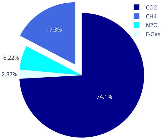
Figure 1.
GHG emissions distribution recorded in 2019 IPCC report [5].
The recent Green AI initiative focuses on the exploitation of cutting-edge technologies, such as deep learning, in order to monitor environmental data and provide processes for the development of more sustainable AI solutions [11]. To that end, climate parameters’ monitoring can be considerably benefited by the advent of recurrent neural networks (RNNs), given their proven efficacy in recent time-series estimation challenges [12,13]. More specifically, recurrent architectures have been proposed in order to add a recursive structure to the conventional deep neural network (DNN) models [14,15]. Hence, RNNs benefitted from their cumulative property that emerges from the observation of previous inputs. However, the common RNNs suffered from the vanishing gradient problem [16], which led to the development of more sophisticated recurrent cells introducing internal memory with gated structures. Amongst the proposed cells, the long short-term memory (LSTM) [17] and the gated recurrent unit (GRU) [18] form two of the most widespread ones given their proven efficacy in a wide range of challenging applications, including natural language processing [19], speech recognition [20], emotion estimation [21], anomaly detection [22], as well as environmental data processing [23,24,25,26,27]. To that end, internal memory’s gates learn to combine, forget and/or pass received information to the following layers. The LSTM cell includes more gates than the GRU one, a fact that usually renders it more efficient in complex and long sequences but, at the same time, they are more computationally expensive [28]. Given the advent of RNNs, their exploitation in the field of environmental forecasting is already visible. LSTM models have been investigated for the prediction of marine environmental information from publicly available industrial databases [24]. Similar architectures have been utilized for the prediction of noise in urban environments [25], as well as GHG emissions prediction in smart homes [26] and, recently, emission of in specific regions [27].
However, the contemporary data collected from the Sentinel-5P mission provide descriptive and accurate measurements regarding the daily profile of GHG around the globe and can be exploited with cutting-edge technologies to provide enhanced forecasting performances. Until now, forecasting of GHG concentration can be conducted only on a local scale due to the limited available measurements of a commons sensory system, thus rendering it difficult to compare against different regions around the globe, constituting an open research gap. As an example, methane concentration forecasting constitutes an active field of research that has been already investigated at a smaller scale [29,30]. Bearing that in mind, a recent work has turned its focus to concentration to monitor the pollution profile of Europe during the Coronavirus outbreak [31]. Hence, our motivation originates from such interest, driven also by the urging need to limit methane emissions at a global scale, in order to reduce the anthropogenic GHGs effect. To achieve that, we exploit the most recent measuring system, viz., the Copernicus Sentinel-5P, which, to the best of our knowledge, constitutes the only satellite providing methane measurements daily and at a global scale. Meanwhile, we investigate the optimal data-driven architecture that can compensate for competitive forecasting performance and realistic execution time and complexity. The main advantage of such an approach focuses on the concise property of the measurement system along different regions, which enables the development of a unified model for estimating methane concentrations. To that end, the paper at hand contributes to the aforementioned attempt, introducing a complete solution that:
- exploits contemporary data from Sentinel-5P mission, capturing concentration in the most active regions, viz., the areas of Texas, Pennsylvania and West Virginia, through an introduced data acquisition scheme;
- develops a handy tool for processing the extracted data for further analysis;
- provides an efficient algorithm for concentration forecasting using recent history measurements and RNN architectures;
- assesses the performance and the computational complexity of the introduced solution and demonstrates its superiority against other machine learning models.
To the best of our knowledge, this is the first method that exploits Sentinel-5P atmospheric data to provide future estimations with RNNs regarding existing trends in the concentration patterns. At this point, we would like to highlight that the proposed work focuses on the prediction of methane concentration and not its emission. Hence, no specific study regarding the processes that control such measurements is conducted.
The remainder of the paper is structured as follows. Section 2, lists the utilized materials and methods of the system, namely the data acquisition and processing as well as the forecasting model adopted for the experimental studies. In Section 3, we display the validation strategy as well as the experimental and comparative studies conducted to conclude an efficient forecasting system and the validation procedure followed to assess its final performance. Section 4 provides an extensive discussion regarding the application of the proposed system and its computational complexity for real applications, while Section 5 displays the final outcomes of the work and discusses directions for future work.
2. Materials and Methods
The current section describes the case study of this work. It provides general information about the Sentinel-5P mission, its instruments, the monitored atmospheric data as well as the data acquired and exploited by the introduced approach. As stated above, the paper at hand introduces a complete solution for concentration acquisition and forecasting from Sentinel-5P data. Hence, in the current section, we proceed with the description of the individual tools that form this final solution. Firstly, a data processing tool is provided for transforming the satellite data into a time-series format. Then, deep learning techniques are applied to accurately predict future concentration through RNN architectures.
2.1. Sentinel-5P Mission
The Sentinel-5P mission is a result of cooperation between ESA, the European Commission (EC), the Netherlands Space Office (NSO), the industry and the scientific community, consisting of a satellite that carries the tropospheric monitoring instrument (TROPOMI) [32,33]. The main purpose of this mission is to perform atmospheric measurements with a high spatial-temporal resolution concerning air quality, ozone, UV radiation and climate monitoring and forecasting. The Sentinel-5P mission also intends to reduce the gaps in worldwide atmospheric measurements between the SCIAMACHY/Envisat mission (concluded in April 2012), the OMI/AURA mission (estimated to be operational until 2022) and the future Copernicus Sentinel-4 and Sentinel-5 missions. The Sentinel-5P was launched on 13 October 2017 and is the first Copernicus mission dedicated to the monitoring of the atmosphere [7].
It constitutes a low Earth-orbit satellite with a high inclination of approximately and is designed for a seven-year operational lifetime. Its sun-synchronous, near-polar orbit ensures that the surface is always illuminated at the same sun angle. The TROPOMI instrument is the only payload of the Sentinel-5P mission [34]. It constitutes a spectrometer sensing ultraviolet (UV: 270–320 nm), visible (VIS: 310–500 nm), near-infrared (NIR: 675–775 nm) and short-wave infrared (SWIR: 2305–2385 nm) radiation. Hence, it is able to monitor ozone (), methane (), formaldehyde (), aerosol, carbon monoxide (), nitrogen dioxide () and sulfur dioxide () in the atmosphere. It combines state-of-the-art technologies with the strengths of the SCIAMACHY and OMI instruments to provide observations with performances that remain unsatisfied by current space instruments in terms of sensitivity, spectral, spatial and temporal resolution. It maps the global atmosphere with an initial spatial resolution of km, which has been changed to km since August 2019. A wide swath of approximately 2600 km on the earth’s surface provides a typical pixel size of km for all spectral bands, except for the UV1 ( km) and the SWIR bands ( km) [32,33,34].
2.2. Data Acquisition
For the experimental study of the introduced method, we make use of the Sentinel-5P dataset, containing the daily concentration of from 6 August 2019 to 31 December 2020. Daily measurements are provided by the NASA Earth Data (GES DISC) platform, thus, ensuring that our case study is developed and tested on real-world data. Each file of the dataset corresponds to a specific date in a common file format, called network common data form (netCDF). NetCDF files are often adopted for storing multi-dimensional scientific variables, such as concentration, humidity, temperature and pressure. Before the acquisition, the regions of interest have to be defined through their corresponding geographic latitude and longitude values. We have decided to investigate the three States of the USA with the highest levels of concentration, viz., Texas, Pennsylvania and West Virginia. The above selection was driven by recent studies regarding the regions that constitute the center of active research on emission treatment [35,36]. In order to end up with regions of a relatively constant area, Texas has been split into eight equal contiguous sub-regions, leading to ten final regions of interest. This was achieved by setting the latitude and longitude values, for the ten aforementioned regions. After data acquisition, an appropriate processing scheme has been developed to convert netCDF files into time-series for data forecasting (discussed in Section 2.3).
2.3. Data Processing Tool
The measurements of a given date are given in a 2-dimensional matrix called , each cell of which corresponds to a small sampling area defined by the resolution of the measuring instrument. Furthermore, each cell is accompanied by a set of values, including the corresponding latitude and longitude values of the geographical area that it describes, as well as several metadata. Firstly, we employ a common search algorithm to keep all the non- values of the array that lie inside the region of interest r, where and with the number of regions. To achieve that, by checking the latitude and longitude values, we store the estimation of a sampling area, in case this lies inside the r-th region of interest, as shown in Figure 2. Subsequently, the entire set of measurements within the r-th region of interest is exploited to calculate its mean concentration for the t-th day, where a number indicating the index of the day in the sequence. The above procedure is repeated for each day within the range of the sampling period stated in Section 2.2. Thus, we end up with a time-series describing the daily mean concentration in the r-th region. An indicative example of the time-series representation is illustrated in Figure 3. We work similarly for each of the ten areas of interest, i.e., the eight sub-regions of Texas for , West Virginia with and Pennsylvania with .
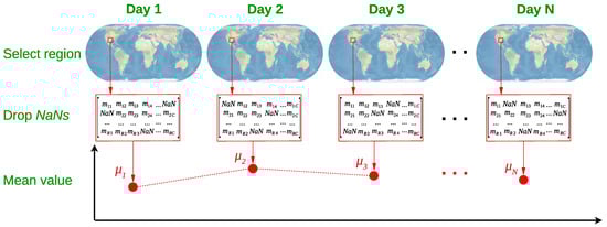
Figure 2.
Data processing tool for the region selection, NaN values discarding and mean value estimation () for the t-th day of measurement.
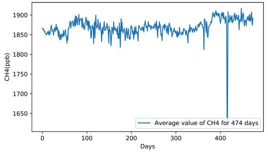
Figure 3.
Time-series representation of daily mean concentration in Texas () for 474 days.
Then, the sequence of each region is standardized so as to display zero mean value and standard deviation equal to 1, a data pre-processing step that leads to proven improvement of the performance in data-driven techniques [37,38]. More specifically, we exploit the common Gaussian normalization equation for each time-series :
where the standardized time-series, the initial one, the mean value of and the standard deviation of . After the extraction of the time-series for each area, we proceed with the creation of smaller sequences of constant length to be fed into RNN architectures for prediction. To that end, the initial time-series of the r-th region is sampled acquiring 51 successive values with a step of 25 until the end of the sequence. At each step, the first values correspond to the sequence that will be fed into the RNN model, while the last one constitutes the value to be predicted. With that having been said, we store the values 0–49 of in the 1-st row of the features matrix F and the 50-th value in the 1-st row of the ground truth one G, as depicted in Figure 4. Accordingly, values 25–74 and 75 are stored in the 2-nd row of F and G, respectively. Following the above policy we gradually store all the sub-sequences of in the sequence dataset , while we similarly split all regions of interest. It should be mentioned that except for values, we have avoided removing any other values, due to the time-dependent nature of the data.
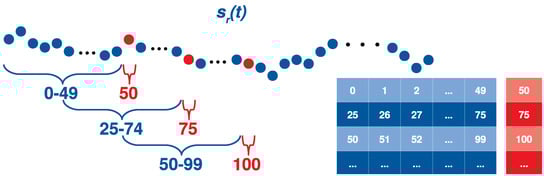
Figure 4.
Time-series division policy: Blue color indicates the input features of the forecasting model while the red one represents the corresponding ground truth labels.
2.4. Methane Concentration Forecasting Model
We propose an efficient methane concentration forecasting model (MCFM) to provide us with the concentration prediction of each extracted sub-sequence, described in Section 2.3. For this purpose, the extracted sub-sequences are fed into an RNN architecture with denoting the number of its hidden layers, namely excluding the input and the output layers. The two well-established cell types of RNNs are investigated, viz., LSTM and GRU cells, as well as a wide range of architectural designs, testing different numbers of hidden layers and neurons. Each layer can display a distinct number of hidden units , where represents the number of the hidden layer. Considering the above, an RNN architecture is written as . The input space of the first hidden layer and, as a result, the input space of the entire model is a single estimation of the daily concentration, while the sequence length is . Similarly, the output layer constitutes a fully connected () layer with only 1 neuron since the desired estimation is a real value , referring to the concentration of the forthcoming day. The rest hidden layers can present different numbers and types of neurons, leading to a wide variety of possible architectures . The parameters N and , along with the cell type are empirically defined, as described in Section 3.3. During training, we attempt to minimize the Mean Squared Error (MSE) loss function, described by the common equation:
where the predicted value, the ground truth and the number of samples. The same MSE metric is utilized to assess the performance of the investigated models.
A summary of the entire methodology is provided in Figure 5, where all the described processes are illustrated in a unified block diagram. As the reader can observe, it is divided into three main pillars, viz., the data acquisition, the data processing tool and the MCFM. Regarding the MCFM pillar, the last process includes the training and assessment of all the machine learning models studied in the scope of the current work and extensively described in Section 3.

Figure 5.
Method overview: the scheme of the introduced methodology is depicted, including all the main processes of the: (a) Data acquisition, (b) Data Processing Tool and (c) Methane Concentration Forecasting Model.
3. Results
In the current section, we describe the entire experimental study conducted, in order to credibly evaluate our method, given that it constitutes the first forecasting model of concentration from the Sentinel-5P data. Firstly, the validation strategy is explained, including the division of the dataset into training and validation data. Then, the experimental setup as well as the parameters to be empirically defined are presented along with the produced experimental results. Finally, we display the performance results of the models of interest derived from our experimental studies and the prediction estimations of the best one compared against the ground-truth curves.
3.1. Validation Strategy
According to Section 2.2, the acquired dataset comprises ten regions, i.e., eight sub-regions of Texas, Pennsylvania and West Virginia. Aiming to investigate the generalization capacities of the forecasting model, we split the dataset into training and evaluation sets, considering in the last set the two most difficult cases. The most common thought would constitute to exploit Texas sub-regions for training and keep the rest two regions for evaluation. Hence, we proceed with an assessment study to quantify the above argument. To achieve that, we pairwise calculate the signal cross-correlation between the regions’ time-series. Thus, the two time-series that present the weakest cross-correlation with the rest ones constitute the most uncorrelated sets of the dataset and will be included in the evaluation set. The obtained results are summarized in Table 1. The reader can verify the anticipated argument that the correlation between the mean inter-correlation of Texas sub-regions is stronger compared against their correlation with Pennsylvania and West Virginia regions. Therefore, we establish the above-mentioned division of the dataset, keeping the regions of Pennsylvania and West Virginia for evaluation purposes.

Table 1.
Obtained cross-correlation values between the sub-regions’ time-series.
3.2. Experimental Setup
As stated in Section 2.4, we investigated several RNN architectures and experimental setups to end up with an efficient prediction model. Besides, the number of hidden layers and neurons are some parameters that can not be optimally defined a priori [39]. For this purpose, we performed a grid search [40] among the several values of the investigated parameters tracking at each step the best evaluation MSE value obtained through the training procedure. The configuration parameters along with their exploration values are the following: (a) learning rate from , (b) cell types , (c) number of hidden layers from and (d) number of hidden neurons from . Given that we keep the best MSE value obtained through a training procedure, we have set a constant number of epochs at 1000 and batch size at 64. The grid search is performed using LSTM layers, while in the case of GRU fewer tests have been conducted since it led to inferior results, stated in Section 3.3. Finally, we employ the broadly known Adam optimizer [41] and the Xavier Glorot weight initialization [42], thanks to their proven efficacy in similar estimation tasks [43,44]. The experiments were conducted on a computer device with an i7 CPU processor and an Nvidia GeForce MX250, 4 GB GPU.
3.3. Model Configuration
Our initial evaluation concerns the definition of the learning rate since it holds a vital role in the efficient convergence of the model. In Figure 6 we observe the curves of the evaluation loss for all three investigated values of the learning rate, keeping the same RNN architecture. The reader can observe the slower but better convergence for in means of achieved MSE values. Although we display the curves of an individual RNN architecture, the same applies to different models, as well. Hence, we excluded the learning rate from the grid search, keeping it constantly at . Subsequently, we proceed with the grid search for the rest three parameters, viz., cell type, number of layers and number of neurons, keeping the best MSE value obtained for each parameters’ configuration during the training procedure. Due to the huge amount of experiments and obtained results, for visualization purposes, we selected to present only seven models of special interest summarized in Table 2, where is either or . More specifically, we chose to include the top-4 models in terms of performance and three more versions that exhibit results worthy of discussion.
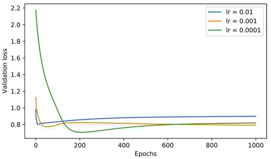
Figure 6.
Loss curves of the forecasting model for different values of the learning rate parameter.
Table 2.
Architectural design of the 7 models selected for discussion with .
In Table 3, lstm-{2, 3, 4, 6} achieve the top-4 MSE values with the last one constituting the best of all. Comparing LSTM models against the corresponding GRU ones, the reader can observe the inferior performance of the latter, which is suggested in all conducted experiments. Hence, after several indicative experiments conducted on GRUs, we decided to perform a grid search only for LSTM models. Lstm-1 depicts a vanilla experiment with only one recurrent hidden neuron to form a baseline for our method. Keeping that in mind, lstm-{5, 7} form two versions that failed to improve baseline results on the evaluation set. On the one hand, lstm-5 appears to lack the capacity to efficiently learn the training data, shaping an indicative instance of under-fitting. On the other hand, lstm-7 consists of one hidden layer with 128 neurons. Paying attention to the noteworthy gap between the training and evaluation loss, we can easily conclude that the model has over-fitted the training data, failing to efficiently generalize. Finally, we indicatively depict the estimation performance of lstm-3 and lstm-6 in Figure 7, shaping the two best solutions. Blue color corresponds to the predictions of lstm-6 and green to the ones of lstm-3. Orange is employed to present the respective ground truth values. Hence, the reader can visually perceive the capacity of each model to predict the actual values of a forthcoming measurement, as well as several inabilities that they display.
Table 3.
Best MSE values obtained from 7 models of interest.
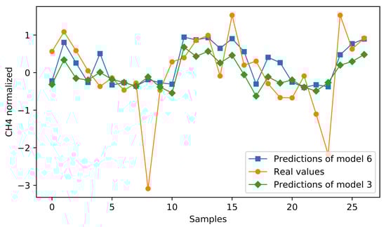
Figure 7.
Predictions of concentration estimated on the evaluation set by the best two forecasting models, i.e., lstm-3 (green) and lstm-6 (blue).
3.4. Comparative Study
Since the Sentinel-5P concentration data have not been exploited yet, we chose to assess our method by comparing it against other state-of-the-art models on the same dataset. In this section, we provide details regarding the conducted comparative study and the obtained results. In particular, we tested several Support Vector Regression (SVR) [45] and DNN architectures and discussed their performance on the concentration forecasting challenge. Similar to the experimental study of the RNNs, the eight regions of Texas were employed for training, while the regions of Pennsylvania and West Virginia were exploited only for evaluation.
As far as the SVR approach is concerned, four different kernels have been tested, viz., linear, polynomial, radial basis function (RBF) and sigmoid. The obtained training and evaluation MSE values are summarized in Table 4. We observe that the best evaluation performance is achieved with the RBF kernel, which is still inferior to the MSE values obtained from the top models of RNNs. Paying attention to the training MSE values, the reader can ascertain that the SVR manages to learn the training data but fails to generalize on the evaluation set. The only exception is the SVR with the sigmoid kernel that seems incapable to solve even the training distribution.
Table 4.
MSE values obtained from SVR utilizing 4 distinct kernels.
Moving to the DNN architectures, we assessed several DNN architectures for different values of hidden layers, , hidden units, with , as well as dropout rates, [46]. Similarly to RNNs, a DNN architecture is denoted as with forming the only addition referring to the utilized dropout rate. Each hidden layer is followed by a ReLU activation function and a batch normalization (BN) layer with trainable mean and standard deviation values [47]. During training, we exploited the same experimental configurations with the RNNs, i.e., we employed the Adam optimizer with a learning rate at , batch size equal to 64. The networks’ weights were initialized adopting the Xavier Glorot initialization method and they were trained for 1000 epochs measuring the obtained training and evaluation MSE values. For each experiment, we kept the best evaluation loss and the corresponding training loss. In Table 5, the top-6 DNN architectures are displayed. Their corresponding evaluation and training best MSE values are summarized in Table 6, where the reader can clearly observe that neither of the presented DNN models achieves competitive results compared against the evaluation MSE values obtained by the RNNs. Moreover, one can discern the quite high training MSE values corresponding to the best evaluation ones. The above indicates that DNNs tend to overfit the training data quite earlier than the RNN ones since for lower training MSE values from the ones presented in Table 6 the evaluation results become worse.
Table 5.
Architectural design of the top-6 DNN models.
Table 6.
Best MSE values obtained from the top-6 DNN models.
4. Discussion
In this section, we discuss the findings of our experimental study and proceed to an extensive description of the efficacy of the investigated models in terms of computational cost and execution time. To begin with, by paying close attention to the results of the LSTM models in Table 3, we found out that more than one architecture can provide us with a quite similar prediction performance. Hence, the initial question regarding the selection of the optimal solution remains open. In fact, it is reasonable to conclude that since more architectures provide satisfactory results, such a selection should include more parameters apart from the prediction performance. The parameters, which mainly bother the community of data scientists and machine learning engineers regarding optimal selection, focus on the complexity and the time efficacy of the designed models.
Bearing in mind the above, we measured the complexity and the execution time of our top RNN and DNN architectures so as to form a well-rounded opinion about the advantages and drawbacks of the developed models. Operational complexity has been measured through the well-established multiply-accumulate (MAC) metric by employing the corresponding function in PyTorch library [48]. At the same time, we also measured the total number of the trainable parameters (Params) of the network. As far as the execution time is concerned, we run ten distinct simple inference tests for each model on our CPU and measured the execution time of each repetition. Finally, we kept the mean value from the ten different execution times of each model. In Table 7 and Table 8, we present the obtained results of the RNN and the DNN models, respectively. Note that, complexity is displayed in and execution time in s.
Table 7.
Complexity and time efficiency metrics for the 7 RNN models of interest.
Table 8.
Complexity and time efficiency metrics for the top-6 DNN models.
In Table 7, we can initially observe that LSTM architectures display a little higher MAC and Params values compared against the corresponding GRU ones, which is highly anticipated given the more complicated structure of the LSTM cell. However, the execution times are quite similar. Paying closer attention to the LSTM models, we discover that the addition of more hidden units in a single recurrent layer gradually increases the MAC and Param values of the network. On the other side, in the case that a deeper RNN is structured with the same amount of total hidden units, the aforementioned complexity metrics can be maintained relatively lower. As an instance, the above fact can be observed in the case of and , where the latter displays about the half number of parameters and MAC value, although they have the same amount of hidden neurons. Yet, a drawback of deeper recurrent networks constitutes the relatively higher execution time required. In DNNs the above metrics are quite similar for most of the architectures, as shown in Table 8. By comparing against the RNN ones, we obviously discern the more lightweight nature of the DNNs, succeeding or lower complexity and execution time rates. Despite that, specific architectures, such as and , achieve top-end performance and, simultaneously, present similar or quite near complexity values to the top-6 DNN models.
Moving one step further, we chose to visually illustrate the summarized behavior of each model so as to better comprehend their advantages and disadvantages. In particular, we display in a common graph the complexity metrics MAC and Params, the execution time, as well as the best evaluation MSE achieved by each model. Due to the high imbalances of the obtained values by each metric both in terms of range and order of magnitude and in order to equally weigh all of the above properties, we standardized the obtained values of each metric. To that end, the obtained results of all the models for a given metric were grouped as a 1-D vector and, then, we applied the Gaussian normalization described in Equation (1). We repeated the same procedure for each one of the four metrics. As a result, we ended up with the graphs in Figure 8, where each sub-figure includes a distinct group of models, viz., LSTM, GRU and DNN architectures. Since all four metrics are inversely proportional to the best performance, models with smaller areas in Figure 8 correspond to the more efficient ones in all four aspects.
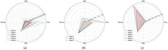
Figure 8.
Visual illustration depicting the summarized performance, complexity and time efficiency of the top RNN and DNN models. (a) top-6 LSTM models; (b) top-3 GRU models; (c) top-6 DNN models.
5. Conclusions
To sum up, the paper at hand constitutes the first attempt to exploit Sentinel-5P data to track and estimate future concentrations of in several geographical regions of interest. Hence, the mitigation of GHG emissions due to anthropogenic processes, like engineering geology ones, can be established. To achieve that, we introduce a handy data processing tool that transforms geographical data provided from the GES DISC platform to region-specific time-series. After several processing steps, we fed the extracted data into an efficient methane concentration forecasting model utilizing RNNs with LSTM and GRU cells. Extensive experimental studies are conducted to conclude the optimal architecture in terms of prediction performance, by measuring the obtained MSE value of each experiment on the evaluation set. In addition, a comparison against other contemporary machine learning models, i.e., SVR and classic DNN architectures, is performed to place the performance of our model within the state-of-the-art. The demonstrated results clearly explain the final selection of the forecasting model design and indicate the promising estimation results achieved, while an illustrative and quantitative discussion regarding the complexity and time efficiency of the examined models is conducted.
The above experimental study designates several key principles regarding the definition of an optimal model that allows data-driven methane concentration forecasting in real and practical scenarios through the available Sentinel-5P products. In particular, the comparison of recurrent architectures against SVR and DNNs highlights the suitability of the first to recognize patterns from sequential data, like daily concentration, and provide accurate future estimations. Furthermore, the specific architecture of the forecasting model is required to be carefully designed based on the needs of the task. To that end, it has been shown that deeper LSTM models are able to enhance prediction performance, yet they tend to highly increase the required execution time. Meanwhile, a larger amount of hidden neurons in a specific recurrent layer increase complexity without benefiting the overall performance. Considering all the above-mentioned principles, the optimal model is defined following the combination of several properties through an aggregated multi-variable performance.
The introduced method turns its focus on the analysis of the daily concentration of and not the processes and human activities that control methane emissions and lead to such concentration values. Anthropogenic methane emissions analysis constitutes a distinct and quite extensive research field attempting to define and forecast the environmental footprint and economic impact of human activities, such as livestock, coal mining, oil and gas production, gas transmission and distribution networks, agricultural waste, wastewater, rice cultivation, etc. [49,50]. On the other hand, our motivation constitutes to treat methane concentration prediction as a time-series forecasting challenge, exploiting the recent sensory capabilities provided by Sentinel-5P.
As part of future work, we aim to further explore the estimation capacities on the Sentinel-5P database, including more regions and/or concentration forecasting. Furthermore, a user-friendly graphical user interface can be developed that projects forthcoming concentration estimations directly on the map of each region of interest, simulating a weather forecast platform.
Author Contributions
Conceptualization, I.K. and A.G.; methodology, T.P. and I.K.; validation, T.P., I.K. and A.G.; formal analysis, I.K.; investigation, T.P.; resources, T.P.; data curation, T.P.; writing—original draft preparation, T.P.; writing—review and editing, I.K. and A.G.; visualization, T.P. and I.K.; supervision, A.G. All authors have read and agreed to the published version of the manuscript.
Funding
This research received no external funding.
Institutional Review Board Statement
Not applicable.
Informed Consent Statement
Not applicable.
Data Availability Statement
In this research, we used prerecorded data collected by the Sentinel-5P mission. The exploited data is publicly available online by the NASA Earth Data (GES DISC) platform (https://disc.gsfc.nasa.gov/, assessed on 21 January 2022).
Conflicts of Interest
The authors declare no conflict of interest.
Abbreviations
The following abbreviations are used in this manuscript:
| GHG | greenhouse gases |
| GCC | global climate change |
| RNN | recurrent neural network |
| DNN | deep neural network |
| LSTM | long short-term memory |
| GRU | gated recurrent unit |
| TROPOMI | tropospheric monitoring instrument |
| MSE | mean squared error |
| MCFM | methane concentration forecasting model |
References
- Nathanail, J.; Banks, V. Climate change: Implications for engineering geology practice. Geol. Soc. Lond. Eng. Geol. Spec. Publ. 2009, 22, 65–82. [Google Scholar] [CrossRef]
- Karl, T.R.; Trenberth, K.E. Modern global climate change. Science 2003, 302, 1719–1723. [Google Scholar] [CrossRef] [PubMed]
- Tuckett, R. Greenhouse gases. In Encyclopedia of Analytical Science; Elsevier: Amsterdam, The Netherlands, 2019; pp. 362–372. [Google Scholar]
- Montzka, S.A.; Dlugokencky, E.J.; Butler, J.H. Non-CO2 greenhouse gases and climate change. Nature 2011, 476, 43–50. [Google Scholar] [CrossRef] [PubMed]
- Shukla, P.; Skea, J.; Calvo Buendia, E.; Masson-Delmotte, V.; Pörtner, H.; Roberts, D.; Zhai, P.; Slade, R.; Connors, S.; Van Diemen, R.; et al. An IPCC special report on climate change, desertification, land degradation, sustainable land management, food security, and greenhouse gas fluxes in terrestrial ecosystems. In Climate Change and Land; IPCC: Geneva, Switzerland, 2019. [Google Scholar]
- Boucher, O.; Friedlingstein, P.; Collins, B.; Shine, K.P. The indirect global warming potential and global temperature change potential due to methane oxidation. Environ. Res. Lett. 2009, 4, 044007. [Google Scholar] [CrossRef]
- Ingmann, P.; Veihelmann, B.; Langen, J.; Lamarre, D.; Stark, H.; Courrèges-Lacoste, G.B. Requirements for the GMES Atmosphere Service and ESA’s implementation concept: Sentinels-4/-5 and-5p. Remote Sens. Environ. 2012, 120, 58–69. [Google Scholar] [CrossRef]
- Balaska, V.; Bampis, L.; Katsavounis, S.; Gasteratos, A. Generating Graph-Inspired Descriptors by Merging Ground-Level and Satellite Data for Robot Localization. Cybern. Syst. 2022, 54, 697–715. [Google Scholar] [CrossRef]
- Krapivin, V.F.; Varotsos, C.A.; Soldatov, V.Y. Simulation results from a coupled model of carbon dioxide and methane global cycles. Ecol. Model. 2017, 359, 69–79. [Google Scholar] [CrossRef]
- Varotsos, C.; Krapivin, V.; Mkrtchyan, F.; Zhou, X. On the effects of aviation on carbon-methane cycles and climate change during the period 2015–2100. Atmos. Pollut. Res. 2021, 12, 184–194. [Google Scholar] [CrossRef]
- Schwartz, R.; Dodge, J.; Smith, N.A.; Etzioni, O. Green ai. Commun. ACM 2020, 63, 54–63. [Google Scholar] [CrossRef]
- Lim, B.; Zohren, S. Time-series forecasting with deep learning: A survey. Philos. Trans. R. Soc. A 2021, 379, 20200209. [Google Scholar] [CrossRef]
- Kansizoglou, I.; Misirlis, E.; Tsintotas, K.; Gasteratos, A. Continuous Emotion Recognition for Long-Term Behavior Modeling through Recurrent Neural Networks. Technologies 2022, 10, 59. [Google Scholar] [CrossRef]
- Yuan, Y.; Shao, C.; Cao, Z.; He, Z.; Zhu, C.; Wang, Y.; Jang, V. Bus dynamic travel time prediction: Using a deep feature extraction framework based on rnn and dnn. Electronics 2020, 9, 1876. [Google Scholar] [CrossRef]
- Kansizoglou, I.; Misirlis, E.; Gasteratos, A. Learning Long-Term Behavior through Continuous Emotion Estimation. In Proceedings of the 14th Pervasive Technologies Related to Assistive Environments Conference, Corfu, Greece, 29 June–2 July 2021; pp. 502–506. [Google Scholar]
- Bengio, Y.; Simard, P.; Frasconi, P. Learning long-term dependencies with gradient descent is difficult. IEEE Trans. Neural Netw. 1994, 5, 157–166. [Google Scholar] [CrossRef] [PubMed]
- Hochreiter, S.; Schmidhuber, J. Long short-term memory. Neural Comput. 1997, 9, 1735–1780. [Google Scholar] [CrossRef] [PubMed]
- Chung, J.; Gulcehre, C.; Cho, K.; Bengio, Y. Empirical evaluation of gated recurrent neural networks on sequence modeling. In Proceedings of the NIPS 2014 Workshop on Deep Learning, Montreal, QC, Canada, 8–13 December 2014. [Google Scholar]
- Azari, E.; Vrudhula, S. An energy-efficient reconfigurable LSTM accelerator for natural language processing. In Proceedings of the 2019 IEEE international conference on big data (Big Data), Los Angeles, CA, USA, 9–12 December 2019; pp. 4450–4459. [Google Scholar]
- Shewalkar, A.; Nyavanandi, D.; Ludwig, S.A. Performance evaluation of deep neural networks applied to speech recognition: RNN, LSTM and GRU. J. Artif. Intell. Soft Comput. Res. 2019, 9, 235–245. [Google Scholar] [CrossRef]
- Kansizoglou, I.; Bampis, L.; Gasteratos, A. An Active Learning Paradigm for Online Audio-Visual Emotion Recognition. IEEE Trans. Affect. Comput. 2019, 13, 756–768. [Google Scholar] [CrossRef]
- Niu, Z.; Yu, K.; Wu, X. LSTM-based VAE-GAN for time-series anomaly detection. Sensors 2020, 20, 3738. [Google Scholar] [CrossRef]
- Kim, K.; Kim, D.K.; Noh, J.; Kim, M. Stable forecasting of environmental time series via long short term memory recurrent neural network. IEEE Access 2018, 6, 75216–75228. [Google Scholar] [CrossRef]
- Wen, J.; Yang, J.; Jiang, B.; Song, H.; Wang, H. Big data driven marine environment information forecasting: A time series prediction network. IEEE Trans. Fuzzy Syst. 2020, 29, 4–18. [Google Scholar] [CrossRef]
- Zhang, X.; Zhao, M.; Dong, R. Time-series prediction of environmental noise for urban IoT based on long short-term memory recurrent neural network. Appl. Sci. 2020, 10, 1144. [Google Scholar] [CrossRef]
- Riekstin, A.C.; Langevin, A.; Dandres, T.; Gagnon, G.; Cheriet, M. Time series-based GHG emissions prediction for smart homes. IEEE Trans. Sustain. Comput. 2018, 5, 134–146. [Google Scholar] [CrossRef]
- Kumari, S.; Singh, S.K. Machine learning-based time series models for effective CO2 emission prediction in India. Environ. Sci. Pollut. Res. 2022, 1–16. [Google Scholar] [CrossRef]
- Yamak, P.T.; Yujian, L.; Gadosey, P.K. A comparison between arima, lstm, and gru for time series forecasting. In Proceedings of the 2019 2nd International Conference on Algorithms, Computing and Artificial Intelligence, Sanya, China, 20–22 December 2019; pp. 49–55. [Google Scholar]
- Demirkan, D.C.; Duzgun, H.S.; Juganda, A.; Brune, J.; Bogin, G. Real-Time Methane Prediction in Underground Longwall Coal Mining Using AI. Energies 2022, 15, 6486. [Google Scholar] [CrossRef]
- Meng, X.; Chang, H.; Wang, X. Methane concentration prediction method based on deep learning and classical time series analysis. Energies 2022, 15, 2262. [Google Scholar] [CrossRef]
- Vîrghileanu, M.; Săvulescu, I.; Mihai, B.A.; Nistor, C.; Dobre, R. Nitrogen Dioxide (NO2) Pollution monitoring with Sentinel-5P satellite imagery over Europe during the coronavirus pandemic outbreak. Remote Sens. 2020, 12, 3575. [Google Scholar] [CrossRef]
- Veefkind, J.; Aben, I.; McMullan, K.; Förster, H.; De Vries, J.; Otter, G.; Claas, J.; Eskes, H.; De Haan, J.; Kleipool, Q.; et al. TROPOMI on the ESA Sentinel-5 Precursor: A GMES mission for global observations of the atmospheric composition for climate, air quality and ozone layer applications. Remote Sens. Environ. 2012, 120, 70–83. [Google Scholar] [CrossRef]
- de Vries, J.; Voors, R.; Ording, B.; Dingjan, J.; Veefkind, P.; Ludewig, A.; Kleipool, Q.; Hoogeveen, R.; Aben, I. TROPOMI on ESA’s Sentinel 5p ready for launch and use. In Proceedings of the Fourth International Conference on Remote Sensing and Geoinformation of the Environment (RSCy2016), Paphos, Cyprus, 4–8 April 2016; Volume 9688, p. 96880B. [Google Scholar]
- Kleipool, Q.; Ludewig, A.; Babić, L.; Bartstra, R.; Braak, R.; Dierssen, W.; Dewitte, P.J.; Kenter, P.; Landzaat, R.; Leloux, J.; et al. Pre-launch calibration results of the TROPOMI payload on-board the Sentinel-5 Precursor satellite. Atmos. Meas. Tech. 2018, 11, 6439–6479. [Google Scholar] [CrossRef]
- Townsend-Small, A.; Hoschouer, J. Direct measurements from shut-in and other abandoned wells in the Permian Basin of Texas indicate some wells are a major source of methane emissions and produced water. Environ. Res. Lett. 2021, 16, 054081. [Google Scholar] [CrossRef]
- Ren, X.; Hall, D.L.; Vinciguerra, T.; Benish, S.E.; Stratton, P.R.; Ahn, D.; Hansford, J.R.; Cohen, M.D.; Sahu, S.; He, H.; et al. Methane emissions from the Marcellus Shale in Southwestern Pennsylvania and Northern West Virginia based on airborne measurements. J. Geophys. Res. Atmos. 2019, 124, 1862–1878. [Google Scholar] [CrossRef]
- Oikonomou, K.M.; Kansizoglou, I.; Manaveli, P.; Grekidis, A.; Menychtas, D.; Aggelousis, N.; Sirakoulis, G.C.; Gasteratos, A. Joint-Aware Action Recognition for Ambient Assisted Living. In Proceedings of the 2022 IEEE International Conference on Imaging Systems and Techniques (IST), Kaohsiung, Taiwan, 21–23 June 2022; pp. 1–6. [Google Scholar]
- Mehedi, M.A.A.; Khosravi, M.; Yazdan, M.M.S.; Shabanian, H. Exploring Temporal Dynamics of River Discharge using Univariate Long Short-Term Memory (LSTM) Recurrent Neural Network at East Branch of Delaware River. Hydrology 2022, 9, 202. [Google Scholar] [CrossRef]
- Kansizoglou, I.; Bampis, L.; Gasteratos, A. Do neural network weights account for classes centers? IEEE Trans. Neural Netw. Learn. Syst. 2022. [Google Scholar] [CrossRef]
- Pontes, F.J.; Amorim, G.; Balestrassi, P.P.; Paiva, A.; Ferreira, J.R. Design of experiments and focused grid search for neural network parameter optimization. Neurocomputing 2016, 186, 22–34. [Google Scholar] [CrossRef]
- Kingma, D.P.; Ba, J. Adam: A Method for Stochastic Optimization. In Proceedings of the 3rd International Conference on Learning Representations, San Diego, CA, USA, 7–9 May 2015. [Google Scholar]
- Glorot, X.; Bengio, Y. Understanding the difficulty of training deep feedforward neural networks. In Proceedings of the International Conference on Artificial Intelligence and Statistics, Sardinia, Italy, 13–15 May 2010; pp. 249–256. [Google Scholar]
- Kansizoglou, I.; Bampis, L.; Gasteratos, A. Deep feature space: A geometrical perspective. IEEE Trans. Pattern Anal. Mach. Intell. 2021, 44, 6823–6838. [Google Scholar] [CrossRef] [PubMed]
- Chang, Z.; Zhang, Y.; Chen, W. Effective adam-optimized LSTM neural network for electricity price forecasting. In Proceedings of the 2018 IEEE 9th International Conference on Software Engineering and Service Science (ICSESS), Beijing, China, 23–25 November 2018; pp. 245–248. [Google Scholar]
- Drucker, H.; Burges, C.J.; Kaufman, L.; Smola, A.; Vapnik, V. Support vector regression machines. Adv. Neural Inf. Process. Syst. 1997, 9, 155–161. [Google Scholar]
- Srivastava, N.; Hinton, G.; Krizhevsky, A.; Sutskever, I.; Salakhutdinov, R. Dropout: A simple way to prevent neural networks from overfitting. J. Mach. Learn. Res. 2014, 15, 1929–1958. [Google Scholar]
- Ioffe, S.; Szegedy, C. Batch normalization: Accelerating deep network training by reducing internal covariate shift. In Proceedings of the International Conference on Machine Learning, Lille France, 6–11 July 2015; pp. 448–456. [Google Scholar]
- Paszke, A.; Gross, S.; Massa, F.; Lerer, A.; Bradbury, J.; Chanan, G.; Killeen, T.; Lin, Z.; Gimelshein, N.; Antiga, L.; et al. Pytorch: An imperative style, high-performance deep learning library. Adv. Neural Inf. Process. Syst. 2019, 32, 8026–8037. [Google Scholar]
- Höglund-Isaksson, L. Global anthropogenic methane emissions 2005–2030: Technical mitigation potentials and costs. Atmos. Chem. Phys. 2012, 12, 9079–9096. [Google Scholar] [CrossRef]
- Jackson, R.B.; Saunois, M.; Bousquet, P.; Canadell, J.G.; Poulter, B.; Stavert, A.R.; Bergamaschi, P.; Niwa, Y.; Segers, A.; Tsuruta, A. Increasing anthropogenic methane emissions arise equally from agricultural and fossil fuel sources. Environ. Res. Lett. 2020, 15, 071002. [Google Scholar] [CrossRef]


Disclaimer/Publisher’s Note: The statements, opinions and data contained in all publications are solely those of the individual author(s) and contributor(s) and not of MDPI and/or the editor(s). MDPI and/or the editor(s) disclaim responsibility for any injury to people or property resulting from any ideas, methods, instructions or products referred to in the content. |
© 2023 by the authors. Licensee MDPI, Basel, Switzerland. This article is an open access article distributed under the terms and conditions of the Creative Commons Attribution (CC BY) license (https://creativecommons.org/licenses/by/4.0/).