Abstract
Understanding the process of earthquake preparation is of utmost importance in mitigating the potential damage caused by seismic events. That is why the study of seismic precursors is fundamental. However, the community studying non-seismic precursors relies on measurements, methods, and theories that lack a causal relationship with the earthquakes they claim to predict, generating skepticism among classical seismologists. Nonetheless, in recent years, a group has emerged that seeks to bridge the gap between these communities by applying fundamental laws of physics, such as the application of the second law of thermodynamics in multiscale systems. These systems, characterized by describing irreversible processes, are described by a global parameter called thermodynamic fractal dimension, denoted as . A decrease in indicates that the system starts seeking to release excess energy on a macroscopic scale, increasing entropy. It has been found that the decrease in prior to major earthquakes is related to the increase in the size of microcracks and the emission of electromagnetic signals in localized zones, as well as the decrease in the ratio of large to small earthquakes known as the b-value. However, it is still necessary to elucidate how , which is also associated with the roughness of surfaces, relates to other rupture parameters such as residual energy, magnitude, or fracture energy. Hence, this work establishes analytical relationships among them. Particularly, it is found that larger magnitude earthquakes with higher residual energy are associated with smoother faults. This indicates that the pre-seismic processes, which give rise to both seismic and non-seismic precursor signals, must also be accompanied by changes in the geometric properties of faults. Therefore, it can be concluded that all types of precursors (seismic or non-seismic), changes in fault smoothness, and the occurrence of earthquakes are different manifestations of the same multiscale dissipative system.
1. Introduction
The study of pre-earthquake physics holds significant relevance in our efforts to safeguard lives and infrastructure from the destructive impact of seismic events. Extensive research has been conducted, focusing on pre-earthquake measurements, such as groundwater level variations, electromagnetic signals, ionospheric variations, seismic clustering, radon liberation, other gas seeps emissions, or thermal radiation, that offer promising indications of a potential link to impending earthquakes [1,2,3,4,5,6,7,8,9,10,11,12,13,14,15,16,17,18,19,20,21,22,23,24,25]. Particularly, these studies highlight the presence of anomalous data during abnormal periods compared to normal background conditions. Nevertheless, it is crucial to recognize that the majority of these studies have primarily focused on establishing spatial and temporal correlations between the observed anomalies and the occurrence of earthquakes.
Although there are studies linking measurements to earthquake magnitude [9,20,26,27,28,29,30], the crucial question of actual causation, which represents the fundamental link between the measured signals and the underlying physics of earthquake rupture, is addressed by only a limited number of researchers within the pre-earthquake signal community [31,32,33,34,35,36]. This gap in our understanding has generated concerns and skepticism within the seismological community, as the reliability and predictive capabilities of pre-earthquake measurements are called into question [37,38]. This skepticism has made it challenging to overcome the prevailing paradigm that denies the existence of pre-earthquake phenomena [39]. To bridge this gap, considerable attention has been directed toward experiments conducted on rock samples, offering valuable insights into the behavior of pre-failure physics [40,41,42,43,44,45,46,47,48,49,50,51]. These studies have explored various phenomena, such as multiscale cracking, rock electrification, changes in acoustic emissions, increases in internal damage, or alterations in strain and stress [52,53,54]. It is thought that the knowledge gained from these rock sample experiments could be extrapolated to understand large-scale lithospheric dynamics.
Significant progress has been achieved in the integration of pre-earthquake signals of the lithosphere with seismic rupture parameters, employing the principles of multiscale thermodynamics and entropy production of rocks [34,35]. A crucial parameter in this framework is the thermodynamic fractal dimension, which accounts for the dissipation of energy across different scales, and specifically characterizes the distribution of multiscale cracking within materials. Notably, the generation of multiscale cracking indicates the dissipation of energy preceding impending earthquakes, marking the culmination of the seismic cycle [36]. This critical stage, which garners significant attention in pre-earthquake signal research, allows for the interpretation of anomalous measurements as manifestations of irreversible processes and impending earthquake occurrence. In this line, Venegas-Aravena et al., 2022 [34] found a relation between the large-scale entropy change to the expected earthquake magnitude. Additionally, Venegas-Aravena and Cordaro 2023 [36] suggested that the multiscale properties of lithospheric dynamics such as the thermodynamic fractal dimension could be linked to fault properties such as the b-value, which indicates the ratio between the larger and smaller earthquakes in a given zone.
In that line, one notable consequence of large-scale entropy production is the emergence of smoother fault surfaces [35,36]. This is relevant because seismological studies describe the fault interface and the seismic source as heterogenous [55,56,57], implying that friction coefficients depend on the roughness of the surface. For example, rougher surfaces are related to higher friction coefficients as well as smooth surfaces host lower friction coefficients [58]. That is why large slips are more related to smoother faults [59,60]. In that sense, the smoothing of faults indicates the release of accumulated energy and a reduction in resistance to energy storage in multiple seismic cycles [61,62,63]. To comprehensively understand fault properties, including earthquake magnitude, it becomes essential to establish a connection between fault smoothing and the global parameters of the system. Multiscale thermodynamics provides a suitable framework for analyzing fault behavior and linking it to pre-earthquake signals. In line with these considerations, the present work utilizes a multiscale thermodynamic approach to investigate the relationship between pre-earthquake signals and fault properties. In that line, Section 2 of this study delves into the intricacies of the principles of multiscale thermodynamics and its application to the understanding of the seismic background. Building upon this foundation, Section 3 explores the relationship between two crucial aspects of fault properties: seismic magnitude and fault geometry. Moving forward, Section 4 investigates the connection between multiscale thermodynamics and fracture energy. The discussion section is in Section 5. Here, the focus shifts to the relationship between fault properties, multiscale thermodynamics, and other pre-seismic processes. Finally, Section 6 presents the conclusions drawn from the findings of the study.
2. Multiscale Thermodynamics
In the context of multiscale cracking, the study of energy dissipation processes is essential to understand the complex behavior of materials under stress. Cracks in rocks, resulting from external loads, exhibit a multiscale nature as they propagate across different length scales [64,65]. These cracking processes are inherently dissipative, reflecting the irreversible release of accumulated energy within the material [66]. To quantitatively analyze and describe such dynamics, a thermodynamic framework is needed. Recent work on multiscale thermodynamics provides this framework, offering insights into entropy production and the thermodynamic fractal dimension as measures of energy dissipation and complexity. One of the key equations in multiscale thermodynamics work relates the thermodynamic fractal dimension () to the multiscale entropy production balance [35]:
where represents the thermodynamic fractal dimension, which characterizes the complexity of the cracking process. The constant is associated with the scaling factor by the relation , reflecting the relationship between different length scales. is the size of the smallest components of the system and , the multiscale entropy production balance, quantifies the interplay between macroscopic () and microscopic () entropy productions. It captures the relative contribution of entropy production at different scales and provides a measure of the overall energy dissipation in the system. According to Venegas-Aravena et al., 2022 [35], the parameter can be expressed as:
where is the Euclidean dimension. By merging Equation (2) into Equation (1), it can be concluded that:
where which corresponds to the exponential term in Equation (2). The equation enables an investigation into how the dominance of macroscopic or microscopic entropy production impacts the thermodynamic fractal dimension. When the macroscopic entropy production dominates (resulting in a larger value of ), it implies a stronger influence of the dissipation at larger scales, leading to a decrease in the thermodynamic fractal dimension. Conversely, when the microscopic entropy production dominates, the thermodynamic fractal dimension tends to increase, indicating a stronger influence of the smaller scales in the energy dissipation process.
Cracking in materials, such as rocks or brittle solids, involves the propagation and interaction of cracks at various scales. At the macroscopic level, the overall cracking behavior and energy dissipation can be captured by the macroscopic entropy production (). On the other hand, the microscopic entropy production () represents the entropy production at smaller scales, capturing the contributions from microcracks, grain boundaries, or other microscopic features. These microscale cracks and defects contribute to the dissipation of energy through processes such as crack propagation, dislocation motion, and local stress concentrations.
3. Seismic Moment and Thermodynamic Fractal Dimension
A relationship has been established between the magnitude of an earthquake (Mw) and the rate of entropy change () [34]. This relationship is given by:
where the exponent is . This relationship shows a connection between the dissipative processes associated with entropy change and the generation of seismic activity. That is, Equation (4) implies that as the rate of entropy change () increases, the magnitude of the earthquake () also tends to increase. Furthermore, the value of is influenced by the thermodynamic fractal dimension . When is smaller, closer to 5, diverges, indicating a stronger relationship between the entropy change and earthquake magnitude. On the other hand, as increases, tends to 0, suggesting a weaker coupling between entropy change and earthquake magnitude. It is important to note that the global entropy change, represented by , provides insights into the overall energy release and dissipation processes occurring within the system. This includes both the cracking generation within the medium and the rupture process during an earthquake. This implies that the entropy production is directly related to the rupture process of faults, including the fault roughness. This can be seen after replacing Equation (3) into Equation (4) after considering that :
where . As Equation (5) directly depends on the thermodynamic fractal dimension , which describes the complexity of surfaces, it implies that Equation (5) links the magnitude and the geometrical irregularities of faults. This implies that smoother surfaces, characterized by lower , may be associated with larger magnitude earthquakes. Conversely, more complex, and rough surfaces, represented by higher fractal dimensions, may result in smaller magnitude earthquakes (Figure 1a). In terms of rupture area, Venegas-Aravena et al., 2022 [34] have also shown a relation between entropy change and ruptured area , expressed as follows:
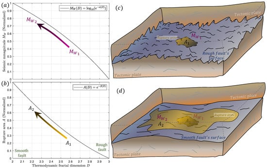
Figure 1.
Relationship between seismic magnitude, rupture area, and the thermodynamic fractal dimension. (a) demonstrates that smaller values of the thermodynamic fractal dimension are associated with larger earthquake magnitudes, while (b) shows how smaller fractal dimensions correspond to larger rupture areas. The thermodynamic fractal dimension also influences fault surface characteristics, with larger values indicating rougher surfaces (c), whereas smaller fractal dimensions result in smoother fault surfaces (d).
Just as Equation (5), Equation (6) can be formulated in relation to the thermodynamic fractal dimension as follows:
where . Equation (7) highlights the connection between the ruptured area and the fault’s irregularities, where the thermodynamic fractal dimension () serves as a measure of the system, encompassing the fault roughness within this context. Additionally, Equation (7) states that smoother faults, resulting from reductions in microscopic stresses or increases in macroscopic stresses, are associated with larger rupture areas (Figure 1b). This equation implies that larger earthquakes are generated in areas characterized by smoother surfaces. While Equations (4)–(7) emerge from the application of multiscale thermodynamics, further exploration is necessary to provide a more comprehensive seismological description of the rupture process and its relationship to fault surfaces. For instance, Figure 1c offers a visual representation highlighting the relationship between the thermodynamic fractal dimension and fault surface characteristics. In this schematic, the yellow area represents the rupture zone, depicting that larger thermodynamic fractal dimensions are associated with rough fault surfaces, smaller ruptured area, and in consequence, smaller magnitude. In contrast, Figure 1d presents a schematic of a fault with a smaller thermodynamic fractal dimension. The schematic representation of a fault surface shown in this figure appears smoother, without the jagged features present in the schematic representation shown in Figure 1c. A smaller fractal dimension corresponds to smoother fault surfaces. Interestingly, faults with smoother surfaces and a smaller fractal dimension exhibit larger rupture area. Consequently, they also tend to generate greater seismic magnitudes, as indicated by the expanded yellow area in the diagram.
4. Fracture Energy
The fracture energy, denoted as , is a measure of the energy required to propagate an earthquake rupture and extend it further within the medium. The value of depends on various factors, including the material properties and the nature of the fracture process [67]. In terms of material properties, different compositions and regimes, such as brittle or ductile behavior, can significantly affect the fracture energy. Ductile materials are generally more resistant to fracture and require a larger amount of energy to propagate the rupture [68]. In contrast, brittle materials exhibit lower fracture energy, as they are more prone to sudden and catastrophic failure [69,70,71]. Interestingly, both brittle and ductile regimes are characterized by relatively small fractal dimensions, resulting in smoother surfaces [69,70]. Smoother surfaces indicate a lower degree of complexity or roughness, as described by the fractal dimension [35]. This can be attributed to the nature of the fracture process in these materials, which tends to generate relatively uniform and well-defined fracture surfaces. On the other hand, composite materials, which consist of a combination of different constituents, exhibit rougher surfaces and tend to have larger fractal dimensions [67]. The presence of multiple materials with different properties introduces heterogeneity and increases the complexity of the fracture surfaces. Figure 2a provides a schematic representation that illustrates the variation of the fractal dimension across different material types as shown by Williford (1988) [69]. Specifically, it shows that brittle and ductile materials tend to exhibit smoother crack surfaces. On the other hand, composite materials display a larger fractal dimension, indicating more irregular and complex crack surfaces. Figure 2b serves as a schematic representation that further elucidates the relationship described in Figure 2a.
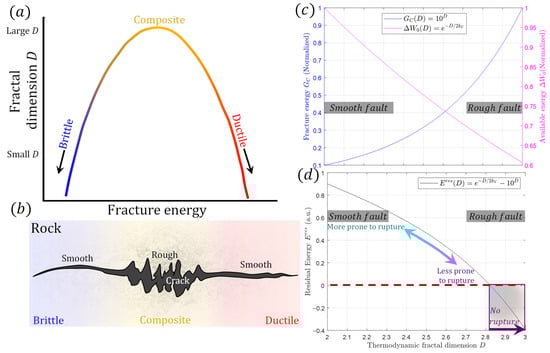
Figure 2.
The figure presents a comprehensive analysis of the dependence of the fractal dimension on material composition and regime. (a) Schematic representation illustrating how the fractal dimension varies according to different material types. Brittle and ductile materials exhibit smoother crack surfaces, while composite materials have a larger fractal dimension; (b) Schematic representation of the relationship described in (a); (c) Demonstrates the interplay between available energy (magenta line) and fracture energy (blue line), both influenced by the thermodynamic fractal dimension; (d) Analytic depiction of the residual energy, which is the difference between available energy and fracture energy, as a function of the thermodynamic fractal dimension.
According to Ohnaka (2013) [71], there is a relationship between fracture energy and the geometrical irregularities of fault interfaces. The geometrical irregularities on faults are characterized by a parameter called . Ohnaka (2013) [72] suggests that materials with smoother fault interfaces have smaller values of and, therefore, require less fracture energy to propagate the rupture. In contrast, materials with rougher fault interfaces have larger values of , resulting in a higher fracture energy requirement to spread the rupture. This can be seen as:
where is a proportional factor and represent a material-dependent constant. If is considerably larger for ductile materials compared to brittle materials, it implies that the same amount of geometrical irregularity () or roughness will result in a higher fracture energy () for ductile materials. This is consistent with the observation that ductile materials can absorb more energy due to their ability to accommodate greater plastic deformation and exhibit higher fracture energy, even with similar levels of smoothness on fault interfaces. Thus, Equation (8) implies that the absence of significant roughness reduces the resistance to rupture propagation, resulting in lower energy requirements.
The fracture energy plays an important role in the generation of earthquakes. For instance, according to Noda et al., 2021 [73], earthquakes are more likely to occur in zones where the residual energy () is positive. This energy is defined as the difference between the available energy , which is partly produced by stress accumulation, and the fracture energy:
Equation (9) does not directly address the concept of fault smoothing or roughness. However, it can draw a connection based on the underlying mechanisms. For example, the fractal dimension is proportional to the logarithm of the roughness: [74]. Equivalently, . This in Equation (8) leads to being written in function of as . In that sense, the increase of geometrical roughness implies the increase of fractal dimension and the increase of as shown Figure 2c (blue line). This into Equation (9) leads to Equation:
where is a constant. Equation (10) means that when a fault surface is smoother, with fewer geometric irregularities or asperities, it requires less energy to propagate the rupture (i.e., lower fracture energy). This means that the energy released during an earthquake is relatively higher compared to the energy needed for fault motion. As a result, the residual energy tends to be positive. In contrast, if the fault surface has more irregularities or roughness, it requires more energy to propagate the rupture (i.e., higher fracture energy). This leads to a lower release of energy during the earthquake relative to the energy needed for fault motion. In such cases, the residual energy may be negative or close to zero and could result in no earthquake generation. Therefore, it can be inferred that smoother fault surfaces, associated with lower fracture energy, are more likely to result in positive residual energy, indicating a higher potential for seismic activity. On the other hand, rougher fault surfaces, associated with higher fracture energy, may lead to lower residual energy and a reduced likelihood of earthquakes.
Therefore, the reduction in fracture energy can lead to an increase in the area characterized by positive residual energy. In other words, more regions become capable of sustaining earthquake propagation due to the lower energy threshold required for rupture. As a result, the areas with reduced fracture energy can increase the areas of potential seismic rupture compared to the pre-smoothing condition. This expansion of the area with positive residual energy increases the overall potential for larger earthquakes to occur.
The available energy is dependent on a function that describes the initial stress states [73,75], which represents the macroscopic stress states (). By utilizing the relationship between macroscopic () and microscopic () stress change balance, expressed as , where [36], the macroscopic stress change can be written as , where . Thus, after temporal integration, the available energy can be described in terms of the thermodynamic fractal dimension as follows:
This equation shows that the macroscopic available energy decreases as the faults are rougher (magenta line in Figure 2c). Here, it is important to note that the rougher surfaces imply greater degree of irregularity and complexity at the small scale. This implies that the stress concentration phenomena are primarily localized and occur on the microscale, resulting in the increase of small-scale available energy. In that sense, Equation (11) offers a complement perspective such as the decrease of the large-scale available energy. By combining Equations (10) and (11), the residual energy in terms of is
The relationship between the thermodynamic fractal dimension and residual energy provides a valuable insight into the seismic activity of faults. Specifically, Equation (12) and Figure 2d indicate that smaller values of are associated with larger residual energy values, while larger values of correspond to negative values of residual energy. The implication of this relationship is that faults with smoother surfaces and smaller values of have the potential to host larger amounts of residual energy. Consequently, they may have a higher likelihood of generating future earthquakes. In contrast, rough faults with larger values of are less likely to accumulate substantial residual energy, resulting in negative values which indicates a fault that is less prone to rupture.
Equations (5), (7), and (12) demonstrate that smaller values of the thermodynamic fractal dimension are correlated with larger areas, magnitudes, and residual energies. Consistent with this, Figure 3a illustrates the relationship between residual energy and the rupture area. Figure 3a confirms that as the residual energy increases, the area prone to rupture also increases. This relationship is captured by the best-fit curve, which correlates residual energy and the area prone to rupture through Equation (13).
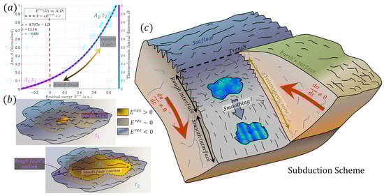
Figure 3.
(a) Relationship between the rupture area and residual energy . The segmented line represents the best second-order power fit. The color bar indicates the thermodynamic fractal dimension; (b) Schematic representation of the relationship depicted in (a) for times and . The yellow area highlights regions prone to rupture. Notably, for smoother surfaces, the area prone to rupture is larger at compared to ; (c) Schematic representation of subduction. The shallow sections are characterized by rougher surfaces compared to the deeper sections. Subduction is considered a fault-smoothing mechanism.
Equation (13) and Figure 3a indicate that rough fault surfaces have a lower capacity to store residual energy, resulting in smaller areas prone to rupture. Conversely, smoother fault surfaces allow for a larger portion of the fault to accommodate significant residual energy. In Figure 3b, areas A1 and A2 represent cases for rougher and smoother fault surfaces, respectively. These figures illustrate how smoother surfaces can store more residual energy, leading to larger areas of potential rupture.
5. Discussions
During an earthquake, the process of rupture involves the fracturing and sliding of rock layers along the fault surface. This process necessitates overcoming resistance forces and the release of accumulated stress energy. However, few studies manage to link processes inside faults with non-seismic precursors. In recent decades, there have been numerous efforts to explain earthquake precursor phenomena or anomalies [16,76,77]. These efforts involve the deformation of lithospheric material, chemical reactions, or the migration of fluids. In addition to not being able to physically link these effects to the earthquakes they try to predict, there are two major additional challenges. Firstly, experiments demonstrate that rock electrification can occur even in the absence of macroscopic stress changes [78]. Secondly, none of these explanations can be directly associated with the earthquakes they are supposed to precede because they cannot be linked to basic rupture parameters within faults [38]. In order to incorporate seismicity, numerous efforts have been focused on describing pre-earthquake phenomena using more fundamental tools, such as the entropy change of the lithosphere [34,35,36,79,80,81]. In that line, the framework proposed by [31,33,34,35,36] suggests that fundamental parameters of seismology, such as magnitude, stress drop, fault friction, or changes in b-value, can be linked to precursor measurements when considering the multiscale crack propagation. These small-scale cracks act as pathways for energy dissipation and contribute to the overall change in entropy [34]. The increase of macroscopic entropy, as described by Equations (2) and (3), is associated with a reduction in the thermodynamic fractal dimension (Equation (1)). This reduction in fractal dimension implies smoother fault surfaces or less geometrical irregularities which are associated with lower fracture energy (Equation (8)). As a consequence, the global features of the system, such as the entropy production, the cracking process, and the physical and geometrical faults are linked. Particularly, based on Equations (5), (7), (12) and (13), there exists an analytical relationship among earthquake size, magnitude, residual energy, and the geometric characteristics of faults. This connection suggests that smoother fault surfaces are more likely to produce larger areas of positive residual energy, which, in turn, can give rise to larger earthquakes.
The connection between smooth fault interfaces and large earthquakes finds support in observations of subduction zones. Specifically, studies suggest that significant Chilean earthquakes occurring in subduction zones, like the Valdivia 1960 Mw9.5 earthquake, may be associated with smooth features within the subduction channels [82]. These smooth features result from the extensive accumulation of sediments during the subduction process, which creates fewer resistance barriers [83]. Furthermore, large-scale simulations demonstrate that smoother surfaces have a greater propensity to generate larger ruptures [84]. On the contrary, Equation (8) suggests that rougher faults result in greater fracture energy, which reduces the probability of obtaining positive residual energy. This interpretation of Equations (8) and (12) indicates that rougher faults tend to generate smaller earthquakes, as described by Equation (13). This finding aligns with studies on subduction zones, which have revealed that geometrical irregularities act as barriers to seismic activity [85].
Studies have demonstrated that moderate-to-large earthquakes predominantly occur at deeper zones within subduction areas [86,87,88]. In contrast, the shallow sections of subduction zones serve as reservoirs for stress accumulation, owing to their higher frictional strength which enables the accumulation of larger stress levels in these shallow regions [89,90]. Hence, deeper zones are more susceptible to earthquake rupture. As illustrated in Figure 3a, this condition aligns with smoother fault surfaces. Consequently, from a multiscale thermodynamic perspective, the shallow sections of the subduction zone exhibit rougher surfaces, while the deeper sections display smoother surfaces. This means that less energy is required to initiate and propagate fractures along these smooth fault interfaces. When the fracture energy is lower, it means that a larger portion of the available energy can be utilized to generate seismic activity (Equation (9)). This can lead to an increase in the area of positive residual energy, as more energy is retained in the system after subtracting the fracture energy. The increase in the area of positive residual energy suggests a greater potential for the occurrence of large earthquakes at deeper zones. This scheme suggests that the subduction of the oceanic crust undergoes a smoothing process as the tectonic plate subducts. Figure 3c provides a schematic representation of this smoothing process, illustrating that the deeper interface sections are smoother compared to the shallower sections. In alignment with this idea, Figure 4a–c indicates the process by which stresses can fracture and smooth out jagged interfaces, resulting in the formation of smoother faults. Figure 4a presents a schematic representation inspired by the experiments conducted by Iquebal et al., 2019 [91], illustrating the polishing of rough surfaces (Figure 6 in Ref. [91]). Figure 4a consists of four surfaces. The first one (1) was created using the code by Chen and Yang [92] to generate a random fractal surface. The other surfaces (2, 3, and 4) were generated by progressively truncating the minimum values. In other words, values smaller than a certain number are set to zero, and this minimum value increases progressively, causing the surfaces to become increasingly gray. These numbered stages resemble the progression of the repetitive sliding contacts shown by reference [91], with higher numbers corresponding to more extensive sliding and consequently smoother surfaces. In this context, Figure 4b,c provide a schematic illustration of how spatial irregularities can store stresses, as demonstrated in Figure 2c (magenta line). In cases where the fractal dimension is 3, representing a rougher interface (Figure 4b), the storage of stresses is limited due to the lower resistance offered by the geometry, resulting in the smoothing of these irregularities. Conversely, Figure 4c depicts a smoother surface that offers greater resistance. Consequently, smoother surfaces tend to be characterized by larger areas, such as the one-dimensional distance illustrated in this case. As residual energy is dependent on stresses (Equation (9)), it follows that larger residual energy is associated with larger areas, as shown in Figure 3a and described by Equation (13). This analysis suggests that the deeper sections of subduction faults, characterized by multiple stages of slip or earthquakes, may exhibit smoother surfaces. The smoothing process as a function of the slip discussed above has significant implications for fault dynamics. For instance, as the fault roughness decreases, there is a tendency for the fractal dimension of the slip distribution to also decrease [93]. In addition, as noted by Morad et al., 2022 [94], fault surfaces that exhibit exceptionally smooth characteristics experience minimal stress increases and sustained slip. This particular behavior may contribute to the occurrence of slow slip events within the deeper sections of megathrust faults, as reported by Ito et al., 2007 [95]. Consequently, the presence of slow slip events suggests that the smoothing process, influenced by the cyclic macroscopic loads described in Equation (1), has already taken place during the fault’s precursor phase. Note that there is evidence supporting the slow slip events as a precursor mechanism [96,97,98,99]. This implies that what is commonly referred to as a slow slip is likely the phase in which the fault, aiming to increase entropy and decrease the thermodynamic fractal dimension of the system, starts to slowly be smoothing the fault at the macroscopic scale, thus becoming one of the final mechanisms for releasing the excess energy. Furthermore, the role of the polishing process can be associated with the “Mogi Doughnut” effect, which describes the seismicity surrounding a large rough patch or asperity prior to its eventual rupture or smoothing (representing a major earthquake) [100,101,102]. In this context, the polishing process reveals the presence of smooth zones surrounding the rough patch, as depicted in Figure 4a. Each rupture event acts as a polishing mechanism that reduces the size of the asperity. Consequently, the immediate surrounding zones of a rough patch are smoother and more prone to generating seismic activity. As the thermodynamic fractal dimension () decreases, indicating smoother faults, more sections of the fault become susceptible to ruptures in the zones surrounding the large asperity. Thus, the decrease in the thermodynamic fractal dimension provides an explanation for the “Mogi Doughnut” effect through the concept of the polishing process.
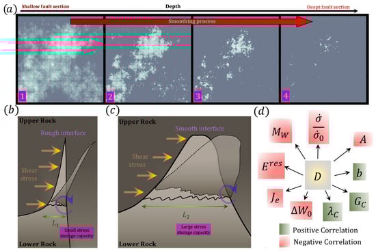
Figure 4.
(a) Smoothing process. The number indicates the number of sliding stages. That is, there are more sliding stages which generate smoother fault at deeper sections of fault. (b,c) shows schematic representation illustrating the stress storage capacity in two cases. Case (b) exhibits a small capacity to hold stresses due to the thin bulge compared to case (c); (c) Schematic representation highlighting the stress storage capacity. In this case, the bulge is thicker, allowing for a larger capacity to hold stresses; (d) Correlation between the thermodynamic fractal dimension and other quantities. Positive correlation is represented by green, while negative correlation is represented by red. Here, the thermodynamic fractal dimension serves as a global parameter controlling various aspects of pre-earthquake physics within the lithosphere.
According to research conducted by Venegas-Aravena and Cordaro (2023) [36], Equation (1) not only relates to the geometric properties of faults such as the smothering of faults, but also to other global parameters, such as the b-value. For example, it has been observed that when studying systems that span multiple scales, the b-value is proportionate to the fractal dimension [36]. However, in certain cases, a complex positive correlation between the b-value and fractal dimension is observed [36]. This discovery aligns with the positive correlation observed between the b-value and fractal dimension in real natural faults [103]. Therefore, the b-value serves as a measure of the stress states within the lithosphere and can indicate zones that are more prone to seismic activity [104]. Specifically, the b-value has been found to exhibit a negative correlation with stress states [105,106]. This implies that as the load on faults increases, the b-value and thermodynamic fractal dimension decrease [35,36]. Consequently, this phenomenon contributes to the smothering of faults, resulting in the accumulation of residual energy and an expansion of the area prone to rupture. The increase in macroscopic entropy production within the system is also associated with the generation of electromagnetic signals prior to earthquakes or macroscopic failure in rock samples [31,34]. In particular, the propagation of multiscale fractures and the movement of charged particles within the newly formed cracks, as a response or dissipation mechanism to the accumulation of external stress, can give rise to electromagnetic emissions, as demonstrated by experiments conducted on rock samples [78,107,108,109].
Furthermore, as the fracture energy decreases, it facilitates the flow of fluids through the fractures, permeating the surrounding rock matrix [110,111]. This migration of fluids can have diverse implications, including the alteration of pore pressure distribution, influencing the stability of the fault zone, and potentially triggering or affecting seismic activity [112]. Consequently, it becomes apparent that the generation of electromagnetic signals, the reduction of fracture energy, fluid migration, fault surface smoothing, increases in the area of positive residual energy, and the occurrence of large earthquakes are interconnected manifestations of the underlying entropy production processes within the Earth’s crust. These processes can be analytically described in terms of the thermodynamic fractal dimension, as summarized in Figure 4d, with the green and red colors indicating positive and negative correlations with the thermodynamic fractal dimension.
Finally, adopting a multiscale perspective reveals that the reduction in thermodynamic dimension signifies a diminished capacity of the lithosphere to release excessive energy at a small scale, such as through minor cracks. Consequently, the system strives for release on progressively larger scales. This phenomenon facilitates the development of larger cracks, establishing additional pathways for fluid migration, thereby potentially causing phenomena like heightened surface temperature or the liberation of trapped gases. Furthermore, these enlarged cracks contribute to intensified levels of anomalous electromagnetic signals. Concurrently, a decrease in the b-value and the smoothing of faults can occur, potentially linked to the occurrence of slow slip events, resulting in an expanded area of positive residual energy. When energy dissipation remains inefficient at this level, the predominant mechanism shifts to macroscopic rupture, ultimately culminating in an earthquake on a larger scale.
6. Conclusions
The main conclusions are listed below:
- The relationship between the magnitude of earthquakes and thermodynamic fractal dimension was established.
- The increases of large-scale entropy production generate the reduction of geometrical irregularities which leads to larger earthquake magnitudes.
- The large-scale entropy production reduces the fracture energy which increases the probability of generating larger ruptures.
- Smoother surfaces found at the deeper sections of subduction faults are more prone to generating heightened seismic activity.
- Subduction can be seen as a mechanism that contributes to the smoothing of faults because it increases macroscopic entropy production.
- Non-seismic earthquake signals are also a manifestation of this entropy change in the system. This means that the system attempts to release the excess energy through the generation of cracks, which can serve as pathways for fluid migration. This can result in changes in ground temperature or the release of gases trapped underground. Additionally, the increase in entropy causes a decrease in b-value and thermodynamic fractal dimension, while also smoothing the faults, thereby reducing the resistance to earthquake generation. This can lead to precursor seismicity.
- Both the geometry of faults and the stored stresses are heterogeneous. Therefore, future studies should focus on establishing how the smoothing process occurs in faults, both in natural settings and laboratory experiments, while other precursor signals are being produced.
Author Contributions
P.V.-A. proposed the core idea, mathematical development, figures, and initial draft of the project. E.G.C. contributed to the scientific discussions of the work. All authors have read and agreed to the published version of the manuscript.
Funding
This research received no external funding.
Data Availability Statement
Not applicable.
Acknowledgments
P.V.-A. would like to thank ANID and PUC for their constant support in the development of science in Chile. P.V.-A. and E.C. would like to express their gratitude to the support staff at the Observatorios de Radiación Cósmica y Geomagnetismo.
Conflicts of Interest
The authors declare no conflict of interest.
References
- Bleier, T.; Dunson, C.; Alvarez, C.; Freund, F.; Dahlgren, R. Correlation of pre-earthquake electromagnetic signals with laboratory and field rock experiments. Nat. Hazards Earth Syst. Sci. 2010, 10, 1965–1975. [Google Scholar] [CrossRef]
- Potirakis, S.M.; Minadakis, G.; Eftaxias, K. Relation between seismicity and pre-earthquake electromagnetic emissions in terms of energy, information and entropy content. Nat. Hazards Earth Syst. Sci. 2012, 12, 1179–1183. [Google Scholar] [CrossRef]
- Petraki, E.; Nikolopoulos, D.; Nomicos, C.; Stonham, J.; Cantzos, D.; Yannakopoulos, P.; Kottou, S. Electromagnetic Pre-earthquake Precursors: Mechanisms, Data and Models—A Review. J. Earth Sci. Clim. Chang. 2015, 6, 250. [Google Scholar] [CrossRef]
- Sanchez-Dulcet, F.; Rodríguez-Bouza, M.; Silva, H.G.; Herraiz, M.; Bezzeghoud, M.; Biagi, P.F. Analysis of observations backing up the existence of VLF and ionospheric TEC anomalies before the Mw6.1 earthquake in Greece, January 26 2014. Phys. Chem. Earth 2015, 85–86, 150–166. [Google Scholar] [CrossRef]
- Schekotov, A.; Hayakawa, M. Seismo-meteo-electromagnetic phenomena observed during a 5-year interval around the 2011 Tohoku earthquake. Phys. Chem. Earth 2015, 85–86, 167–173. [Google Scholar] [CrossRef]
- Scoville, J.; Heraud, J.; Freund, F. Pre-earthquake magnetic pulses. Nat. Hazards Earth Syst. Sci. 2015, 15, 1873–1880. [Google Scholar] [CrossRef]
- Cordaro, E.G.; Venegas, P.; Laroze, D. Latitudinal variation rate of geomagnetic cutoff rigidity in the active Chilean convergent margin. Ann. Geophys. 2018, 36, 275–285. [Google Scholar] [CrossRef]
- Ouzounov, D.; Pulinets, S.; Hattori, K.; Taylor, P. Pre-Earthquake Processes: A Multidisciplinary Approach to Earthquake Prediction Studies. Am. Geophys. Union Geophys. Monogr. Ser. 2018, 12, 1–365. [Google Scholar] [CrossRef]
- De Santis, A.; Marchetti, D.; Pavón-Carrasco, F.J.; Cianchini, G.; Perrone, L.; Abbattista, C.; Alfonsi, L.; Amoruso, L.; Campuzano, S.A.; Carbone, M.; et al. Precursory worldwide signatures of earthquake occurrences on Swarm satellite data. Sci. Rep. 2019, 9, 20287. [Google Scholar] [CrossRef]
- Nakagawa, K.; Yu, Z.-Q.; Berndtsson, R.; Kagabu, M. Analysis of earthquake-induced groundwater level change using self-organizing maps. Environ. Earth Sci. 2019, 78, 445–455. [Google Scholar] [CrossRef]
- Wei, C.; Lu, X.; Zhang, Y.; Guo, Y.; Wang, Y. A time-frequency analysis of the thermal radiation background anomalies caused by large earthquakes: A case study of the wenchuan 8.0 earthquake. Adv. Space Res. 2019, 65, 435–445. [Google Scholar] [CrossRef]
- Sabbarese, C.; Ambrosino, F.; Chiodini, G.; Giudicepietro, F.; Macedonio, G. Continuous radon monitoring during seven years of volcanic unrest at Campi Flegrei caldera (Italy). Sci. Rep. 2020, 10, 9551–9610. [Google Scholar] [CrossRef] [PubMed]
- Warden, S.; MacLean, L.; Lemon, J.; Schneider, D. Statistical Analysis of Pre-earthquake Electromagnetic Anomalies in the ULF Range. J. Geophys. Res. 2020, 125, e2020JA027955. [Google Scholar] [CrossRef]
- Xiong, P.; Long, C.; Zhou, H.; Battiston, R.; Zhang, X.; Shen, X. Identification of Electromagnetic Pre-Earthquake Perturbations from the DEMETER Data by Machine Learning. Remote Sens. 2020, 12, 3643. [Google Scholar] [CrossRef]
- Cordaro, E.G.; Venegas, P.; Laroze, D. Long-term magnetic anomalies and their possible relationship to the latest greater Chilean earthquakes in the context of the seismo-electromagnetic theory. Nat. Hazards Earth Syst. Sci. 2021, 21, 1785–1806. [Google Scholar] [CrossRef]
- Freund, F.; Ouillon, G.; Scoville, J.; Sornette, D. Earthquake precursors in the light of peroxy defects theory: Critical review of systematic observations. Eur. Phys. J. Spec. Top. 2021, 230, 7–46. [Google Scholar] [CrossRef]
- Mehdi, S.; Shah, M.; Naqvi, N.A. Lithosphere atmosphere ionosphere coupling associated with the 2019 Mw 7.1 California earthquake using GNSS and multiple satellites. Environ. Monit. Assess. 2021, 193, 501. [Google Scholar] [CrossRef]
- Vasilev, A.; Tsekov, M.; Petsinski, P.; Gerilowski, K.; Slabakova, V.; Trukhchev, D.; Botev, E.; Dimitrov, O.; Dobrev, N.; Parlichev, D. New Possible Earthquake Precursor and Initial Area for Satellite Monitoring. Front. Earth Sci. 2021, 8, 586283. [Google Scholar] [CrossRef]
- Heavlin, W.D.; Kappler, K.; Yang, Y.; Fan, M.; Hickey, J.; Lemon, J.; MacLean, L.; Bleier, T.; Riley, P.; Schneider, D. Case-Control Study on a Decade of Ground-Based Magnetometers in California Reveals Modest Signal 24–72 hr Prior to Earthquakes. J. Geophys. Res. 2022, 127, e2022JB024109. [Google Scholar] [CrossRef]
- Marchetti, D.; De Santis, A.; Campuzano, S.A.; Zhu, K.; Soldani, M.; D’Arcangelo, S.; Orlando, M.; Wang, T.; Cianchini, G.; Di Mauro, D.; et al. Worldwide Statistical Correlation of Eight Years of Swarm Satellite Data with M5.5+ Earthquakes: New Hints about the Preseismic Phenomena from Space. Remote Sens. 2022, 14, 2649. [Google Scholar] [CrossRef]
- Peleli, S.; Kouli, M.; Vallianatos, F. Satellite-Observed Thermal Anomalies and Deformation Patterns Associated to the 2021, Central Crete Seismic Sequence. Remote Sens. 2022, 14, 3413. [Google Scholar] [CrossRef]
- Anyfadi, E.-A.; Gentili, S.; Brondi, P.; Vallianatos, F. Forecasting Strong Subsequent Earthquakes in Greece with the Machine Learning Algorithm NESTORE. Entropy 2023, 25, 797. [Google Scholar] [CrossRef]
- Bulusu, J.; Arora, K.; Singh, S.; Edara, A. Simultaneous electric, magnetic and ULF anomalies associated with moderate earthquakes in Kumaun Himalaya. Nat. Hazards 2023, 116, 3925–3955. [Google Scholar] [CrossRef]
- Shah, M.; Shahzad, R.; Ehsan, M.; Ghaffar, B.; Ullah, I.; Jamjareegulgarn, P.; Hassan, A.M. Seismo Ionospheric Anomalies around and over the Epicenters of Pakistan Earthquakes. Atmosphere 2023, 14, 601. [Google Scholar] [CrossRef]
- Fidani, C. The Conditional Probability of Correlating East Pacific Earthquakes with NOAA Electron Bursts. Appl. Sci. 2022, 12, 10528. [Google Scholar] [CrossRef]
- Rikitake, T. Earthquake precursors in Japan: Precursor time and detectability. Tectonophysics 1987, 136, 265–282. [Google Scholar] [CrossRef]
- Moriya, T.; Mogi, T.; Takada, M. Anomalous pre-seismic transmission of VHF-band radio waves resulting from large earthquakes, and its statistical relationship to magnitude of impending earthquakes. Geophys. J. Int. 2010, 180, 858–870. [Google Scholar] [CrossRef]
- Han, P.; Zhuang, J.; Hattori, K.; Chen, C.-H.; Febriani, F.; Chen, H.; Yoshino, C.; Yoshida, S. Assessing the Potential Earthquake Precursory Information in ULF Magnetic Data Recorded in Kanto, Japan during 2000–2010: Distance and Magnitude Dependences. Entropy 2020, 22, 859. [Google Scholar] [CrossRef]
- Li, M.; Yang, Z.; Song, J.; Zhang, Y.; Jiang, X.; Shen, X. Statistical Seismo-Ionospheric Influence with the Focal Mechanism under Consideration. Atmosphere 2023, 14, 455. [Google Scholar] [CrossRef]
- Zhang, Y.; Wang, T.; Chen, W.; Zhu, K.; Marchetti, D.; Cheng, Y.; Fan, M.; Wang, S.; Wen, J.; Zhang, D.; et al. Are There One or More Geophysical Coupling Mechanisms before Earthquakes? The Case Study of Lushan (China) 2013. Remote Sens. 2023, 15, 1521. [Google Scholar] [CrossRef]
- Venegas-Aravena, P.; Cordaro, E.G.; Laroze, D. A review and upgrade of the lithospheric dynamics in context of the seismoelectromagnetic theory. Nat. Hazards Earth Syst. Sci. 2019, 19, 1639–1651. [Google Scholar] [CrossRef]
- Martinelli, G.; Plescia, P.; Tempesta, E. “Pre-Earthquake” Micro-Structural Effects Induced by Shear Stress on α-Quartz in Laboratory Experiments. Geosciences 2020, 10, 155. [Google Scholar] [CrossRef]
- Venegas-Aravena, P.; Cordaro, E.G.; Laroze, D. The spatial–temporal total friction coefficient of the fault viewed from the perspective of seismo-electromagnetic theory. Nat. Hazards Earth Syst. Sci. 2020, 20, 1485–1496. [Google Scholar] [CrossRef]
- Venegas-Aravena, P.; Cordaro, E.G.; Laroze, D. Natural Fractals as Irreversible Disorder: Entropy Approach from Cracks in the Semi Brittle-Ductile Lithosphere and Generalization. Entropy 2022, 24, 1337. [Google Scholar] [CrossRef]
- Venegas-Aravena, P.; Cordaro, E.; Laroze, D. Fractal Clustering as Spatial Variability of Magnetic Anomalies Measurements for Impending Earthquakes and the Thermodynamic Fractal Dimension. Fractal Fract. 2022, 6, 624. [Google Scholar] [CrossRef]
- Venegas-Aravena, P.; Cordaro, E.G. Analytical Relation between b-Value and Electromagnetic Signals in Pre-Macroscopic Failure of Rocks: Insights into the Microdynamics’ Physics Prior to Earthquakes. Geosciences 2023, 13, 169. [Google Scholar] [CrossRef]
- Hough, S.E. Predicting the Unpredictable: The Tumultuous Science of Earthquake Prediction; Princeton University Press: Princeton, NJ, USA, 2010. [Google Scholar]
- Picozza, P.; Conti, L.; Sotgiu, A. Looking for Earthquake Precursors from Space: A Critical Review. Front. Earth Sci. 2021, 9, 676775. [Google Scholar] [CrossRef]
- Szakács, A. Precursor-Based Earthquake Prediction Research: Proposal for a Paradigm-Shifting Strategy. Front. Earth Sci. 2021, 8, 548398. [Google Scholar] [CrossRef]
- Surkov, V.V.; Molchanov, O.A.; Hayakawa, M. Pre-earthquake ULF electromagnetic perturbations as a result of inductive seismomagnetic phenomena during microfracturing. J. Atmos. Sol.-Terr. Phys. 2003, 65, 31–46. [Google Scholar] [CrossRef]
- Eftaxias, K.; Potirakis, S.M. Current challenges for pre-earthquake electromagnetic emissions: Shedding light from micro-scale plastic flow, granular packings, phase transitions and self-affinity notion of fracture process. Nonlinear Process. Geophys. 2013, 20, 771–792. [Google Scholar] [CrossRef]
- Kamiyama, M.; Sugito, M.; Kuse, M.; Schekotov, A.; Hayakawa, M. On the precursors to the 2011 Tohoku earthquake: Crustal movements and electromagnetic signatures. Geomat. Nat. Hazards Risk 2014, 7, 471–492. [Google Scholar] [CrossRef]
- Matsuyama, K.; Katsuragi, H. Power law statistics of force and acoustic emission from a slowly penetrated granular bed. Nonlinear Process. Geophys. 2014, 21, 1–8. [Google Scholar] [CrossRef][Green Version]
- Contoyiannis, Y.; Potirakis, S.M.; Eftaxias, K.; Contoyianni, L. Tricritical crossover in earthquake preparation by analyzing preseismic electromagnetic emissions. J. Geodyn. 2015, 84, 40–54. [Google Scholar] [CrossRef]
- Enomoto, Y.; Yamabe, T.; Okumura, N. Causal mechanisms of seismo-EM phenomena during the 1965–1967 Matsushiro earthquake Swarm. Sci. Rep. 2017, 7, 44774. [Google Scholar] [CrossRef]
- Niccolini, G.; Lacidogna, G.; Carpinteri, A. Fracture precursors in a working girder crane: AE natural-time and b-value time series analyses. Eng. Fract. Mech. 2019, 210, 393–399. [Google Scholar] [CrossRef]
- Frid, V.; Rabinovitch, A.; Bahat, D. Earthquake forecast based on its nucleation stages and the ensuing electromagnetic radiations. Phys. Lett. A 2020, 384, 126102. [Google Scholar] [CrossRef]
- Frid, V.; Rabinovitch, A.; Bahat, D. Seismic moment estimation based on fracture induced electromagnetic radiation. Eng. Geol. 2020, 274, 105692. [Google Scholar] [CrossRef]
- Wang, J.-H. Piezoelectricity as a mechanism on generation of electromagnetic precursors before earthquakes. Geophys. J. Int. 2020, 224, 682–700. [Google Scholar] [CrossRef]
- Klyuchkin, V.N.; Novikov, V.A.; Okunev, V.I.; Zeigarnik, V.A. Comparative analysis of acoustic and electromagnetic emissions of rocks. IOP Conf. Ser. Earth Environ. Sci. 2021, 929, 012013. [Google Scholar] [CrossRef]
- Agalianos, G.; Tzagkarakis, D.; Loukidis, A.; Pasiou, E.D.; Triantis, D.; Kourkoulis, S.K.; Stavrakas, I. Correlation of Acoustic Emissions and Pressure Stimulated Currents recorded in Alfas-stone specimens under three-point bending. The role of the specimens’ porosity: Preliminary results. Procedia Struct. Integr. 2022, 41, 452–460. [Google Scholar] [CrossRef]
- Triantis, D.; Pasiou, E.D.; Stavrakas, I.; Kourkoulis, S.K. Hidden Affinities Between Electric and Acoustic Activities in Brittle Materials at Near-Fracture Load Levels. Rock Mech. Rock Eng. 2022, 55, 1325–1342. [Google Scholar] [CrossRef]
- Stergiopoulos, C.; Stavrakas, I.; Triantis, D.; Vallianatos, F.; Stonham, J. Predicting fracture of mortar beams under three-point bending using non-extensive statistical modeling of electric emissions. Phys. A Stat. Mech. Its Appl. 2015, 419, 603–611. [Google Scholar] [CrossRef]
- Kourkoulis, S.K.; Pasiou, E.D.; Dakanali, I.; Stavrakas, I.; Triantis, D. Notched marble plates under direct tension: Mechanical response and fracture. Constr. Build. Mater. 2018, 167, 426–439. [Google Scholar] [CrossRef]
- Ruiz, J.; Baumont, D.; Bernard, P.; Berge-Thierry, C. Combining a Kinematic Fractal Source Model with Hybrid Green’s Functions to Model Broadband Strong Ground Motion. Bull. Seismol. Soc. Am. 2013, 103, 3115–3130. [Google Scholar] [CrossRef]
- Hinkle, A.R.; Nöhring, W.G.; Leute, R.; Junge, T.; Pastewka, L. The emergence of small-scale self-affine surface roughness from deformation. Sci. Adv. 2020, 6, eaax0847. [Google Scholar] [CrossRef] [PubMed]
- Aghababaei, R.; Brodsky, E.E.; Molinari, J.F.; Chandrasekar, S. How roughness emerges on natural and engineered surfaces. MRS Bull. 2022, 47, 1229–1236. [Google Scholar] [CrossRef]
- Svahn, F.; Kassman-Rudolphi, Å.; Wallén, E. The influence of surface roughness on friction and wear of machine element coatings. Wear 2003, 254, 1092–1098. [Google Scholar] [CrossRef]
- Brodsky, E.E.; Gilchrist, J.J.; Sagy, A.; Collettini, C. Faults smooth gradually as a function of slip. Earth Planet. Sci. Lett. 2011, 302, 185–193. [Google Scholar] [CrossRef]
- Goebel, T.H.W.; Brodsky, E.E.; Dresen, G. Fault Roughness Promotes Earthquake-Like Aftershock Clustering in the Lab. Geophys. Res. Lett. 2023, 50, e2022GL101241. [Google Scholar] [CrossRef]
- Sagy, A.; Brodsky, E.E.; Axen, G.J. Evolution of fault-surface roughness with slip. Geology 2007, 35, 283–286. [Google Scholar] [CrossRef]
- Candela, T.; Renard, F.; Schmittbuhl, J.; Bouchon, M.; Brodsky, E.E. Fault slip distribution and fault roughness. Geophys. J. Int. 2011, 187, 959–968. [Google Scholar] [CrossRef]
- Eijsink, A.M.; Kirkpatrick, J.D.; Renard, F.; Ikari, M.J. Fault surface morphology as an indicator for earthquake nucleation potential. Geology 2022, 50, 1356–1360. [Google Scholar] [CrossRef]
- Shiari, B.; Miller, R.E. Multiscale modeling of crack initiation and propagation at the nanoscale. J. Mech. Phys. Solids 2016, 88, 35–49. [Google Scholar] [CrossRef]
- Hedayati, R.; Hosseini-Toudeshky, H.; Sadighi, M.; Mohammadi-Aghdam, M.; Zadpoor, A.A. Multiscale modeling of fatigue crack propagation in additively manufactured porous biomaterials. Int. J. Fatigue 2018, 113, 416–427. [Google Scholar] [CrossRef]
- Slepyan, S.I. Principle of maximum energy dissipation rate in crack dynamics. J. Mech. Phys. Solids 1993, 41, 1019–1033. [Google Scholar] [CrossRef]
- Xie, H. Fractals in Rock Mechanics, 1st ed.; CRC Press: Boca Raton, FL, USA, 1993. [Google Scholar]
- Lu, C. Some notes on the study of fractals in fracture. In Proceedings of 5th Australasian Congress on Applied Mechanics, ACAM 2007, Brisbane, Australia, 10–12 December 2007; pp. 234–239. [Google Scholar]
- Williford, R.E. Multifractal fracture. Scr. Metall. 1988, 22, 1749–1754. [Google Scholar] [CrossRef]
- Williford, R.E. Scaling similarities between fracture surfaces, energies, and a structure parameter. Scr. Metall. 1988, 22, 197–200. [Google Scholar] [CrossRef]
- Bai, Y.; Lu, C.; Ke, F.; Xia, M. Evolution induced catastrophe. Phys. Lett. A 1994, 185, 196–200. [Google Scholar] [CrossRef]
- Ohnaka, M. The Physics of Rock Failure and Earthquakes; Cambridge University Press: Cambridge, UK, 2013. [Google Scholar] [CrossRef]
- Noda, A.; Saito, T.; Fukuyama, E.; Urata, Y. Energy-based scenarios for great thrust-type earthquakes in the Nankai trough subduction zone, southwest Japan, using an interseismic slip-deficit model. J. Geophys. Res. Solid Earth 2021, 126, e2020JB020417. [Google Scholar] [CrossRef]
- Underwood, E.E.; Banerji, K. Fractals in fractography. Mater. Sci. Eng. 1986, 80, 1–14. [Google Scholar] [CrossRef]
- Venkataraman, A.; Kanamori, H. Observational constraints on the fracture energy of subduction zone earthquakes. J. Geophys. Res. 2004, 109, B05302. [Google Scholar] [CrossRef]
- Dobrovolsky, I.P.; Gershenzon, N.I.; Gokhberg, M.B. Theory of electrokinetic effects occurring at the final stage in the preparation of a tectonic earthquake. Phys. Earth Planet. Inter. 1989, 57, 144–156. [Google Scholar] [CrossRef]
- Pulinets, S.; Ouzounov, D. Lithosphere–Atmosphere–Ionosphere Coupling (LAIC) model—An unified concept for earthquake precursors validation. J. Asian Earth Sci. 2011, 41, 371–382. [Google Scholar] [CrossRef]
- Loukidis, A.; Tzagkarakis, D.; Kyriazopoulos, A.; Stavrakas, I.; Triantis, D. Correlation of Acoustic Emissions with Electrical Signals in the Vicinity of Fracture in Cement Mortars Subjected to Uniaxial Compressive Loading. Appl. Sci. 2023, 13, 365. [Google Scholar] [CrossRef]
- Ohsawa, Y. Regional Seismic Information Entropy to Detect Earthquake Activation Precursors. Entropy 2018, 20, 861. [Google Scholar] [CrossRef]
- Ramírez-Rojas, A.; Flores-Márquez, E.L.; Sarlis, N.V.; Varotsos, P.A. The Complexity Measures Associated with the Fluctuations of the Entropy in Natural Time before the Deadly México M8.2 Earthquake on 2017. Entropy 2018, 20, 477. [Google Scholar] [CrossRef]
- Posadas, A.; Pasten, D.; Vogel, E.E.; Saravia, G. Earthquake hazard characterization by using entropy: Application to northern Chilean earthquakes. Nat. Hazards Earth Syst. Sci. 2023, 23, 1911–1920. [Google Scholar] [CrossRef]
- Contreras-Reyes, E.; Flueh, E.R.; Grevemeyer, I. Tectonic control on sediment accretion and subduction off south central Chile: Implications for coseismic rupture processes of the 1960 and 2010 megathrust earthquakes. Tectonics 2010, 29, 1–27. [Google Scholar] [CrossRef]
- Contreras-Reyes, E.; Carrizo, D. Control of high oceanic features and subduction channel on earthquake ruptures along the Chile–Peru subduction zone. Phys. Earth Planet. Inter. 2011, 186, 49–58. [Google Scholar] [CrossRef]
- Zielke, O.; Galis, M.; Mai, P.M. Fault roughness and strength heterogeneity control earthquake size and stress drop. Geophys. Res. Lett. 2017, 44, 777–783. [Google Scholar] [CrossRef]
- Menichelli, I.; Corbi, F.; Brizzi, S.; Van Rijsingen, E.; Lallemand, S.; Funiciello, F. Seamount Subduction and Megathrust Seismicity: The Interplay Between Geometry and Friction. Geophys. Res. Lett. 2023, 50, e2022GL102191. [Google Scholar] [CrossRef]
- Lay, T.; Kanamori, H.; Ammon, C.J.; Koper, K.D.; Hutko, A.R.; Ye, L.; Yue, H.; Rushing, T.M. Depth-varying rupture properties of subduction zone megathrust faults. J. Geophys. Res. 2012, 117, 1–21. [Google Scholar] [CrossRef]
- Hayes, G.P.; Herman, M.W.; Barnhart, W.D.; Furlong, K.P.; Riquelme, S.; Benz, H.M.; Bergman, E.; Barrientos, S.; Earle, P.S.; Samsonov, S. Continuing megathrust earthquake potential in Chile after the 2014 Iquique earthquake. Nature 2014, 512, 295–298. [Google Scholar] [CrossRef] [PubMed]
- Melgar, D.; Riquelme, S.; Xu, X.; Baez, J.C.; Geng, J.; Moreno, M. The first since 1960: A large event in the Valdivia segment of the Chilean Subduction Zone, the 2016 M7.6 Melinka earthquake. Earth Planet. Sci. Lett. 2017, 474, 68–75. [Google Scholar] [CrossRef]
- Li, S.; Barnhart, W.D.; Moreno, M. Geometrical and Frictional Effects on Incomplete Rupture and Shallow Slip Deficit in Ramp-Flat Structures. Geophys. Res. Lett. 2018, 45, 8949–8957. [Google Scholar] [CrossRef]
- Moreno, M.; Li, S.; Melnick, D.; Bedford, J.R.; Baez, J.C.; Motagh, M.; Metzger, S.; Vajedian, S.; Sippl, C.; Gutknecht, B.D.; et al. Chilean megathrust earthquake recurrence linked to frictional contrast at depth. Nature Geosci. 2018, 11, 285–290. [Google Scholar] [CrossRef]
- Iquebal, A.S.; Sagapuram, D.; Bukkapatnam, S.T.S. Surface plastic flow in polishing of rough surfaces. Sci. Rep. 2019, 9, 10617. [Google Scholar] [CrossRef]
- Chen, Y.; Yang, H. Numerical simulation and pattern characterization of nonlinear spatiotemporal dynamics on fractal surfaces for the whole-heart modeling applications. Eur. Phys. J. B 2016, 89, 181. [Google Scholar] [CrossRef]
- Bruhat, L.; Klinger, Y.; Vallage, A.; Dunham, E.M. Influence of fault roughness on surface displacement: From numerical simulations to coseismic slip distributions. Geophys. J. Int. 2020, 220, 1857–1877. [Google Scholar] [CrossRef]
- Morad, D.; Sagy, A.; Tal, Y.; Hatzor, Y.H. Fault roughness controls sliding instability. Earth Planet. Sci. Lett. 2022, 579, 117365. [Google Scholar] [CrossRef]
- Ito, Y.; Obara, K.; Shiomi, K.; Sekine, S.; Hirose, H. Slow Earthquakes Coincident with Episodic Tremors and Slow Slip Events. Science 2007, 315, 503–506. [Google Scholar] [CrossRef]
- Ruiz, S.; Metois, M.; Fuenzalida, A.; Ruiz, J.; Leyton, F.; Grandin, R.; Vigny, C.; Madariaga, R.; Campos, J. Intense foreshocks and a slow slip event preceded the 2014 Iquique Mw 8.1 earthquake. Science 2014, 345, 1165–1169. [Google Scholar] [CrossRef]
- Selvadurai, P.A.; Glaser, S.D.; Parker, J.M. On factors controlling precursor slip fronts in the laboratory and their relation to slow slip events in nature. Geophys. Res. Lett. 2017, 44, 2743–2754. [Google Scholar] [CrossRef]
- Voss, N.; Dixon, T.H.; Liu, Z.; Malservisi, R.; Protti, M.; Schwartz, S. Do slow slip events trigger large and great megathrust earthquakes? Sci. Adv. 2018, 4, eaat8472. [Google Scholar] [CrossRef]
- Luo, Y.; Liu, Z. Slow-Slip Recurrent Pattern Changes: Perturbation Responding and Possible Scenarios of Precursor toward a Megathrust Earthquake. Geochem. Geophys. Geosystems 2019, 20, 852–871. [Google Scholar] [CrossRef]
- Mogi, K. Some features of recent seismic activity in and near Japan (2) activity before and after great earthquakes. Bull. Earthq. Res. Inst. 1969, 47, 395–417. [Google Scholar]
- Kanamori, H. The nature of seismicity patterns before large earthquakes. In Earthquake Prediction: An International Review, Maurice Ewing Series; Simpson, D.W., Richards, P.G., Eds.; American Geophysical Union: Washington DC, USA, 1981; Volume 4, pp. 1–19. [Google Scholar] [CrossRef]
- Schurr, B.; Moreno, M.; Tréhu, A.M.; Bedford, J.; Kummerow, J.; Li, S.; Oncken, O. Forming a Mogi Doughnut in the Years Prior to and Immediately Before the 2014 M8.1 Iquique, Northern Chile, Earthquake. Geophys. Res. Lett. 2020, 47, e2020GL088351. [Google Scholar] [CrossRef]
- Cochran, E.S.; Page, M.T.; van der Elst, N.J.; Ross, Z.E.; Trugman, D.T. Fault Roughness at Seismogenic Depths and Links to Earthquake Behavior. Seism. Rec. 2023, 3, 37–47. [Google Scholar] [CrossRef]
- Morales-Yáñez, C.; Bustamante, L.; Benavente, R.; Sippl, C.; Moreno, M. B-value variations in the Central Chile seismic gap assessed by a Bayesian transdimensional approach. Sci. Rep. 2022, 12, 21710. [Google Scholar] [CrossRef] [PubMed]
- Scholz, C.H. On the stress dependence of the earthquake b value. Geophys. Res. Lett. 2015, 42, 1399–1402. [Google Scholar] [CrossRef]
- Dong, L.; Zhang, L.; Liu, H.; Du, K.; Liu, X. Acoustic Emission b Value Characteristics of Granite under True Triaxial Stress. Mathematics 2022, 10, 451. [Google Scholar] [CrossRef]
- Vallianatos, F.; Tzanis, A. Electric Current Generation Associated with the Deformation Rate of a Solid: Preseismic and Coseismic Signals. Phys. Chem. Earth 1998, 23, 933–938. [Google Scholar] [CrossRef]
- Stavrakas, I.; Triantis, D.; Agioutantis, Z.; Maurigiannakis, S.; Saltas, V.; Vallianatos, F.; Clarke, M. Pressure stimulated currents in rocks and their correlation with mechanical properties. Nat. Hazards Earth Syst. Sci. 2004, 4, 563–567. [Google Scholar] [CrossRef]
- Pasiou, E.D.; Triantis, D. Correlation between the electric and acoustic signals emitted during compression of brittle materials. Frat. Ed Integrità Strutt. 2017, 40, 41–51. [Google Scholar] [CrossRef]
- Nelson, R.A. 1—Evaluating Fractured Reservoirs: Introduction. In Geologic Analysis of Naturally Fractured Reservoirs, 2nd ed.; Gulf Professional Publishing: Houston, TX, USA, 2001; pp. 1–100. [Google Scholar] [CrossRef]
- Finkbeiner, T.; Zoback, M.; Flemings, P.; Stump, B. Stress, ore pressure, and dynamically constrained hydrocarbon columns in the South Eugene Island 330 field, northern Gulf of Mexico. AAPG Bull. 2001, 85, 1007–1031. [Google Scholar]
- Donzé, F.V.; Tsopela, A.; Guglielmi, Y.; Henry, P.; Gout, C. Fluid migration in faulted shale rocks: Channeling below active faulting threshold. Eur. J. Environ. Civ. Eng. 2020, 27, 1–15. [Google Scholar] [CrossRef]


Disclaimer/Publisher’s Note: The statements, opinions and data contained in all publications are solely those of the individual author(s) and contributor(s) and not of MDPI and/or the editor(s). MDPI and/or the editor(s) disclaim responsibility for any injury to people or property resulting from any ideas, methods, instructions or products referred to in the content. |
© 2023 by the authors. Licensee MDPI, Basel, Switzerland. This article is an open access article distributed under the terms and conditions of the Creative Commons Attribution (CC BY) license (https://creativecommons.org/licenses/by/4.0/).