Abstract
Fragility curves of retaining walls constitute an efficient tool for the estimation of seismic risk and can be utilized for prevention from potential damage or for immediate decision-making. In this work, fragility curves for cantilever retaining walls of three different heights are proposed, considering cohesionless soil materials. The seismic response of the soil-wall system, in terms of permanent vertical ground displacement of the backfill soil and permanent horizontal displacement of the wall’s base, is estimated by conducting non-linear time history analyses, through the 2D finite element simulation method. Five initial conditions are investigated regarding the value of the global factor of safety (FS) under static conditions. An initial value of FS equal to 1.5 is considered for dry conditions. If the presence of the water table is taken into account, the corresponding FS drops to values ranging from 1.4 to 1.1. Parameters that characterize seismic intensity are evaluated based on criteria, in order to identify the intensity measures that best correlate with the system’s response. Three damage states are adopted, corresponding to minor, moderate, and extensive damage. The approach of combined damage criteria is also investigated. Finally, fragility curves are derived demonstrating the degree of dependency on initial conditions.
1. Introduction
The impact of seismic events on retaining walls along roadway axes can be of major importance, as induced damage can affect the orderly road operation directly and in the long term, not to count fatalities, human injuries, and loss of properties. According to the Geotechnical Extreme Events Reconnaissance (GEER) database, deformations and failures of retaining structures have been reported in historical earthquake events of the past, like the Kobe, Chi-Chi, Iquique, and Cephalonia earthquakes [1,2,3,4], but also in more recent events, such as the earthquake sequence in central Italy in 2016 [5], and Kahramanmaras (Turkey) in 2023 [6]. Therefore, a seismic fragility assessment of such elements is a critical factor that contributes to the prevention and mitigation of the direct loss corresponding to the physical damages of the road network, and the indirect loss related to the long-term reduced functionality [7].
The term of seismic fragility refers to the tendency of an element or system to perform inadequately when subjected to a seismic event. Fragility curves are utilized as a probabilistic measure to assess the seismic performance of an element exposed to risk. They describe the probability of reaching or exceeding predefined damage states, as a function of the intensity of ground shaking. Different methods can be applied for the derivation of fragility curves, namely empirical, based on expert judgment, numerical, and hybrid methods. Empirical fragility curves are derived by collecting data from post-earthquake observations. The difficulties involved in this approach include the comprehensive amount of data required from many seismic events and the estimation of spatial distribution of seismic intensity at various locations. Fragility curves based on expert judgement (e.g., HAZUS, 2004 [8]) are based on experts’ opinion regarding the possible damage of a structure, induced by certain levels of seismic intensity. This approach is characterized by a high level of subjectivity difficult to quantify [9]. Recently, numerical analyses have been widely used, as they provide the ability to model and estimate the seismic response of any type of structure. Finally, hybrid methods result from the combination of the previously mentioned approaches, as they use empirical data from past earthquakes in order to optimize relationships obtained by analytical or judgment-based methods.
In seismic fragility analyses, the possible damage states of the structure are bounded by some predefined limit states. Damage levels, as well as damage indices, are generally linked to the seismic-induced displacements of the structure. In the case of retaining walls, a first reference to failure criteria by defining the horizontal displacement of the wall as a percentage of its height has been made by Prakash et al. (1995) [10]. They proposed the percentage 2% of wall height as a criterion for permissible horizontal displacements, whereas 10% of wall height as a failure criterion. Following this proposal, Huang et al. (2009) [11], investigated the permissible displacements of conventional retaining walls in the scope of internal friction angle mobilization along the potential failure line of the cohesionless backfill. They conducted shaking table tests, as well as seismic displacement analyses utilizing Newmark’s sliding block theory. The results demonstrated that for horizontal displacements up to 2% of wall height, the backfill soil retains its maximum strength, while for displacements greater than 5% of wall height, the friction angle reaches a reduced value, and the soil undergoes residual deformations. The above-mentioned criteria have been introduced to seismic fragility analyses, by means of a damage index. Zamiran & Osouli (2018) [12] adopted the horizontal displacement of the wall as a damage index, assuming the percentages 2%, 5% and 8% of wall height as limit values corresponding to the exceedance of minor, moderate, and extensive damage levels. Cosentini & Bozzoni (2022) [13] and Seo et al. (2022) [14] adopted the limit values of 2%, 5% and 10% for the three damage states, respectively.
Other parameters adopted in the literature as damage indices for fragility analyses of retaining walls are the peak vertical ground displacement of the backfill and the angle of rotation of the wall. Argyroudis et al. (2013) [15] and Seo et al. (2022) [14], used the threshold values of 0.05 m, 0.15 m, and 0.40 m as vertical displacement limit states for minor, moderate, and extensive damage levels, according to the criteria proposed by the research program SYNER-G (2013) [16]. In those cases, the damage states were qualitatively correlated with the serviceability level of the road. Furthermore, the rotation angle was adopted for gravity walls by Cosentini & Bozzoni (2022) [13], calculated as the arc tangent of the ratio of the horizontal displacement to the total wall height. The predefined limit states were equal to the damage criteria proposed by PIANC (2001) [17] for quay walls, i.e., 3° for minor, 5° for moderate, and 8° for extensive damage.
So far, much research has been carried out regarding the derivation of fragility curves for retaining walls along roadways, by using the finite element method (FEM) or finite difference method (FDM) software. Argyroudis et al. (2013) [15] proposed fragility curves for bridge abutments of 6 m and 7.5 m height for soil classes C and D, according to Eurocode 8 [18] by conducting dynamic analyses in FEM software PLAXIS 2D [19]. The proposed fragility curves were compared to observed damage during the Niigata-Chuetsu Oki 2007 earthquake. Zamiran & Osouli (2018) [12] evaluated the seismic response of a 6 m height cantilever retaining wall, considering three different configurations of the backfill cohesion, i.e., 0 kPa, 10 kPa, and 30 kPa. FDM software FLAC 2D [20] was used to determine the seismic response of the wall. The developed fragility curves denoted to what level a difference in cohesion can affect the probability of damage. Cosentini & Bozzoni (2022) [13] proposed fragility curves for two different shapes of gravity retaining walls of 3.6 m, 8 m, and 12 m height, and two configurations of the backfill inclination (0° and 30°). Dynamic analyses were carried out with FDM software FLAC 2D [20]. Following an investigation, peak ground acceleration (PGA) and peak ground velocity (PGV) were selected as the seismic intensity measures that best correlated with the wall’s response, in terms of permanent horizontal displacement and rotation of the wall. Seo et al. (2022) [14], evaluated seismic fragility of 4 m height cantilever retaining walls, for 0°, 10°, and 20° slope angle of the backfill. Considering the four soil classes of the South Korean classification system, site response analyses were carried out to estimate the corresponding ground motions characteristics. The seismic response of the soil-wall system was computed by conducting 2D FDM analyses (FLAC 2D [20]). Fragility curves were proposed as a function of the peak ground acceleration (PGA) and cumulative absolute velocity (CAV).
In the existing research on seismic fragility assessment of retaining walls, only dry backfill conditions have been considered, therefore assuming that the material is well drained. In practice, malfunctioning of drains due to a blockage of the drainage pipe and inadequate maintenance is usually observed. In these cases, the presence of water leads to the increase of lateral pressure against the wall, resulting in larger displacements and a decrease of the safety factor (Fs) as the water table rises to higher levels [21]. This study focuses on the development of novel fragility curves for cantilever retaining walls with cohesionless foundation soil and backfill materials, considering five different initial conditions regarding the value of global factor of safety (Fs) under static conditions. The variation in the values of Fs is due to the change of the water table level behind the wall. In particular, the dimensions of three cantilever retaining walls with different heights are determined, provided that they have a value of Fs = 1.5 under dry conditions. Subsequently, the presence of water table in different levels behind the wall is considered, resulting in the drop of Fs to values equal to 1.4, 1.3, 1.2, and 1.1. Hence, the effect of different initial conditions to the fragility of the soil-wall system is examined, adopting as damage criteria the permanent vertical ground displacement of the backfill soil, the permanent horizontal displacement of the wall’s base, and the approach of combined criteria. An investigation to identify the seismic intensity parameters that satisfactorily correlate with the system’s response is also carried out.
2. Materials and Methods
The objective of this article is the generation of fragility curves for cantilever retaining walls, while investigating to what extent the presence of water table in various levels affects the seismic fragility. Towards this aim, the working stages included (a) the generation of the FE soil-wall system models by selecting the appropriate geometry and parameters of the constitutive models; (b) the 2D dynamic analyses considering five different initial conditions; and (c) the derivation of fragility curves after estimating the requisite parameters of the fragility function. A thorough description of the working stages is presented below.
In order to estimate the seismic response of the cantilever retaining wall, the FEM software PLAXIS 2D [19] was utilized. The initial step involved the creation of the soil-wall model, as shown in Figure 1. The 2D model consists of the cantilever retaining wall, with a geometry within the range of common practice, the backfill soil behind the wall, at the toe of the wall and at its foundation, the soil material that is an extension of the backfill and extends to one meter below the footing level (layer 1), and the underlying soil layer with a thickness of 7 m (layer 2). Bedrock is simulated at the base of the model, so that the compliant base boundary condition required for the dynamic analyses can be applied. Soil layers were considered as non-cohesive materials, with the properties presented in Table 1.
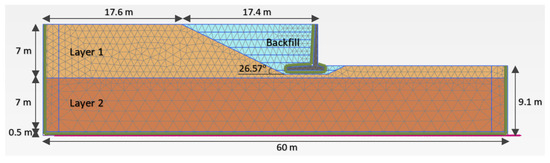
Figure 1.
The 2D soil-wall model regarding the case of R.W.6.

Table 1.
Main parameters of soil and concrete.
A total model width of 60 m was selected, to ensure that the influence of vertical boundaries is limited. Regarding the dimensions of the wall, a parameterization was performed for three different heights of 3 m, 6 m, and 9 m. Opting for wall dimensions that would ensure stability under dry conditions, the “safety calculation” analysis provided by PLAXIS 2D [19] was utilized. This type of analysis implements the phi/c reduction method, that reduces the shear strength parameters tanφ and c until failure occurs. Hence, trial investigations were carried out to identify the exact wall dimensions of the three models R.W.3, R.W.6, and R.W.9, that would result in a value of the global factor of safety under dry conditions equal to 1.5. A schematic view of the retaining wall is depicted in Figure 2, while the selected dimensions of R.W.3, R.W.6, and R.W.9 are presented in Table 2.
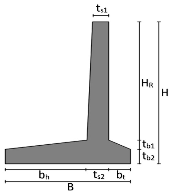
Figure 2.
Schematic view of the retaining wall, where H is the wall height; HR is the stem height; tb2 is the base thickness at the edges; tb1 + tb2 is the base thickness at the stem joint; B is the base width; bh is the heel width; bt is the toe width; ts1 is the stem top thickness; and ts2 is the stem base thickness.
Table 2.
Dimensions of the retaining wall models R.W.3, R.W.6, and R.W.9.
A retaining wall can experience a seismic event anytime during its life. It is not unusual that several years after the construction of a retaining wall (especially at provincial or national mountainous road networks) drainage systems become less efficient, and therefore, the initial conditions of safety can be seriously reduced. This phenomenon is simulated with an increase of the water level behind the retaining wall. To investigate the dependency of seismic fragility on initial conditions, four additional FE models of R.W.3, R.W.6, and R.W.9 were generated, considering the presence of water table at different levels, so that the value of Fs will drop to 1.4, 1.3, 1.2, and 1.1 accordingly. Regarding the pore water pressure, the assumption of hydrostatic conditions has been made. The precise water levels behind the wall (measured from the wall base level), as shown in Table 3, were determined for the three retaining walls individually by conducting trial safety analyses implementing the phi/c reduction method. It is observed that for the unfavorable case of Fs = 1.1, the water table rises to a level equal to 50% times the wall height, for all three cases of retaining walls. Figure 3 indicatively presents the water levels corresponding to the four initial conditions, for the case of R.W.6.
Table 3.
Water table levels behind the walls and the corresponding values of global Fs, regarding the three models R.W.3, R.W.6, and R.W.9.

Figure 3.
Schematic representation of the water levels corresponding to the four different initial conditions Fs = 1.4, 1.3, 1.2, and 1.1, regarding the case of R.W.6.
The defined boundary conditions for the static analyses include a fully fixed base of the model, and normally fixed boundaries at the vertical edges constraining horizontal movement. For the dynamic analyses, free field boundary conditions were defined for lateral boundaries, enabling free field motion, whilst absorbing the reflected waves as they are connected to the main domain through viscous dampers. Concerning the base of the model, the boundary condition of the compliant base was adopted for the dynamic analyses. The compliant base consists of the combination of a viscous boundary in order to have a minimum wave reflection at the base of the model and allows the input of the earthquake motion.
To simulate soil’s behavior, the Hardening Soil small (HSsmall) constitutive model was implemented. HSsmall is an advanced elastic-plastic model that accounts for the soil’s high stiffness in the small strain range, the strain dependency of stiffness, and the stress dependency of stiffness and strength. In HSsmall, the Mohr–Coulomb failure criterion is introduced. The nonlinear behavior of soil is determined by a shear hardening (deviatoric) yield surface, and a cap yield surface that explains the plastic volumetric strain mostly observed in softer types of soil. The soil stiffness is simulated by means of the secant stiffness modulus E50, corresponding to 50% of the ultimate deviatoric stress at the primary loading stage of the triaxial compression test, the oedometric tangent modulus, Eoed, and the elastic modulus for unloading and reloading, namely . During unloading and reloading, the behavior of soil is considered elastic, while the soil stiffness decreases nonlinearly as the number of load cycles increases. In HSsmall, the shear modulus reduction curve is characterized by the small-strain shear modulus G0, and the shear strain γ0.7, at which the secant shear modulus has reduced to 72.2% of G0. The maximum value of G0, was calculated utilizing the relationship:
where is the soil density in kg/m3. The decay of the shear modulus with increasing shear strain, is approximated in PLAXIS 2D by applying relationship (2) that is based on the Hardin-Drnevich [22] equation. According to Bringkreve et al. (2007) [23], the comparison of curves of different types of soil indicated that the value of γ0.7 is between 1–2 × 10⁻⁴, whereas the value of G0 can range from 10 × Gur for soft soils to 2.5 × Gur for harder types of soil, where Gur is the shear modulus for unloading and reloading.
Within the very small strain range, the response of the soil is assumed to be linear elastic. Thus, a Rayleigh damping of 5% was introduced to the model at the target frequencies f1 = 6.7 Hz and f2 = 19 Hz, to account for the realistic viscous characteristics of soil in the dynamic analyses. The target frequencies correspond to the first and the second natural frequencies of the soil deposit, as demonstrated by the Fourier transfer function between the surface and the bedrock level.
The values of the parameters required to determine the constitutive model HSsmall were selected from the experimental triaxial and oedometer test results found in [24]. These parameters are the reference stiffness moduli , and calculated for reference stress pref = 100 kPa, the secant shear modulus at very small strains , the shear strain γ0.7 at which the secant shear modulus has reduced to 72.2% of its initial value, the coefficient m that defines the amount of stiffness dependency on stress level, and the Poisson ratio at unloading-reloading vur. The soil and wall properties adopted for the determination of the constitutive models are demonstrated in Table 4.
Table 4.
Soil and concrete properties of the dynamic analyses model.
The selection of the appropriate element size for mesh discretization is a prerequisite for the proper simulation of wave propagation through soil strata. According to international practice, the maximum dimension lmax of each element should not exceed 10% of the wavelength propagating in the medium. Considering λmin as the wavelength, Vs as the velocity of the shear wave, and fmax as the maximum frequency of the seismic excitation, the maximum permissible element dimension of each soil material was calculated by the relation:
Considering fmax ≈ 12 Hz, for layer 1, the maximum permissible element dimension is equal to 1.67 m, for layer 2, lmax = 2.42 m, for the backfill, lmax = 1.92 m, and for the bedrock, lmax = 6.67 m. The model was discretized, using 15-node triangular elements, that provide a fourth order interpolation for displacements and the numerical integration involves twelve stress points. To properly model the soil-wall interaction, interface elements were used, defined by five pairs of nodes. The interface characteristics were determined based on the adjacent soil by setting the strength reduction factor (Rinter) equal to 0.8. At the first computational stage, initial vertical horizontal effective stresses were calculated. On a second stage, elastic-plastic deformation analysis was carried out. At this point, the backfill was simulated to be constructed per stages of one meter, starting from the wall foundation level. This is a realistic approach as it allows to account for the generated deformations at each individual stage of construction.
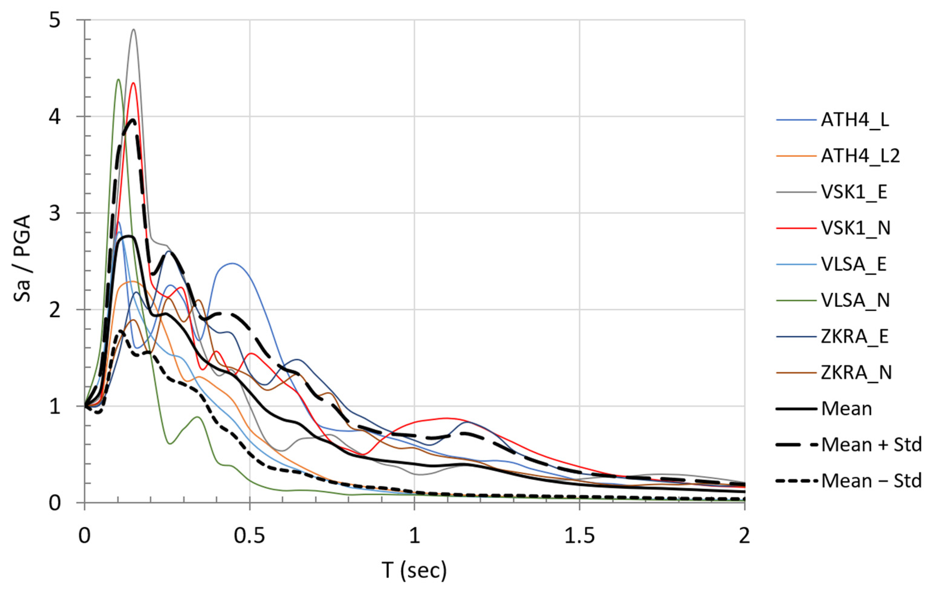
In order to estimate the seismic response of the three wall models, eight real acceleration time histories from five different seismic events were selected, as the strongest seismic motions of the Hellenic database recorded on rock conditions (Margaris et al., 2021 [25]) (Table 5). The normalized acceleration response spectra of the selected records, as well as the mean normalized spectrum ± one standard deviation, are presented in Figure 4. Aiming to correlate the induced displacements with the increasing seismic intensity under free field conditions, the input time histories were scaled to PGA values equal to 0.1 g, 0.2 g, 0.3 g, 0.4 g and 0.5 g. The upper scaling limit of PGA = 0.5 g has been chosen as a probable seismic intensity level in Greece, and precisely in the Region of East Macedonia and Thrace, according to seismic hazard maps proposed in the work of Sotiriadis et al. (2023) [26]. Therefore, 600 dynamic analyses (3 retaining wall models × 40 input motions × 5 initial conditions) and two additional sets of 40 2D soil response analyses were carried out to estimate the values of seismic intensity measures under free field conditions, considering and ignoring the presence of water table, respectively. It should be noted that the aim of this work is the proposal of fragility curves that have a broad implementation area and can be subsequently utilized in conjunction with seismic hazard analysis results concerning specific sites, in order to estimate seismic risk of the corresponding areas. Therefore, record selection was not performed based on spectrum compatibility, as this would have led to limitations regarding the site applicability of the proposed fragility curves. Instead, real acceleration time histories recorded on rock conditions were selected and scaled, following the incremental dynamic analysis method. A similar approach regarding ground motion selection has been followed in the literature by Che et al. (2020) [27], Zamiran and Osouli (2018) [12], and Lesgidis et al. (2017) [28].
Table 5.
Characteristics of input motions used for the dynamic analyses (Margaris et al., 2021 [25]).

Figure 4.
Normalized acceleration response spectra (5% damping ratio) of the selected records, and mean normalized spectrum ± one standard deviation.
To calibrate the soil model and verify the FE seismic analyses results, the response of a one-dimensional (1D) soil column created in PLAXIS was compared with the results obtained from the 1D site response analysis software STRATA [29]. By adopting the soil properties of the 2D model, a 1D soil column was simulated in PLAXIS after applying the boundary condition of tied degrees of freedom at the lateral boundaries. Thus, the nodes at the lateral boundaries of the model would undergo the same displacements and the simulation of 1D wave propagation could be achieved. Moreover, the fundamental frequencies of the three soil-retaining wall models of 3 m, 6 m, and 9 m height were estimated by generating the ratios of the power spectra of the wall stem over the power spectra at the bedrock.
In this study, the permanent horizontal displacement of the wall base (Ux), and the permanent vertical ground displacement of the backfill material (Uy), were selected as damage indices (DI) to be compared with predefined thresholds that express different damage levels. For the horizontal displacement, three threshold values of Ux, expressed as a function of the wall height (0.02 × H m, 0.05 × H m, 0.10 × H m) were assumed [13,14]. Regarding the vertical ground displacement of the backfill, the damage criteria proposed by the research program SYNER-G [16] were adopted, considering three limit values of Uy (0.05 m, 0.15 m, 0.40 m). Based on the different limit states three damage levels were determined, namely minor, moderate, and extensive damage state, that were qualitatively correlated with the road serviceability level according to Argyroudis et al. (2013) [15], as presented in Table 6.
Table 6.
Definition of damage states for retaining walls.
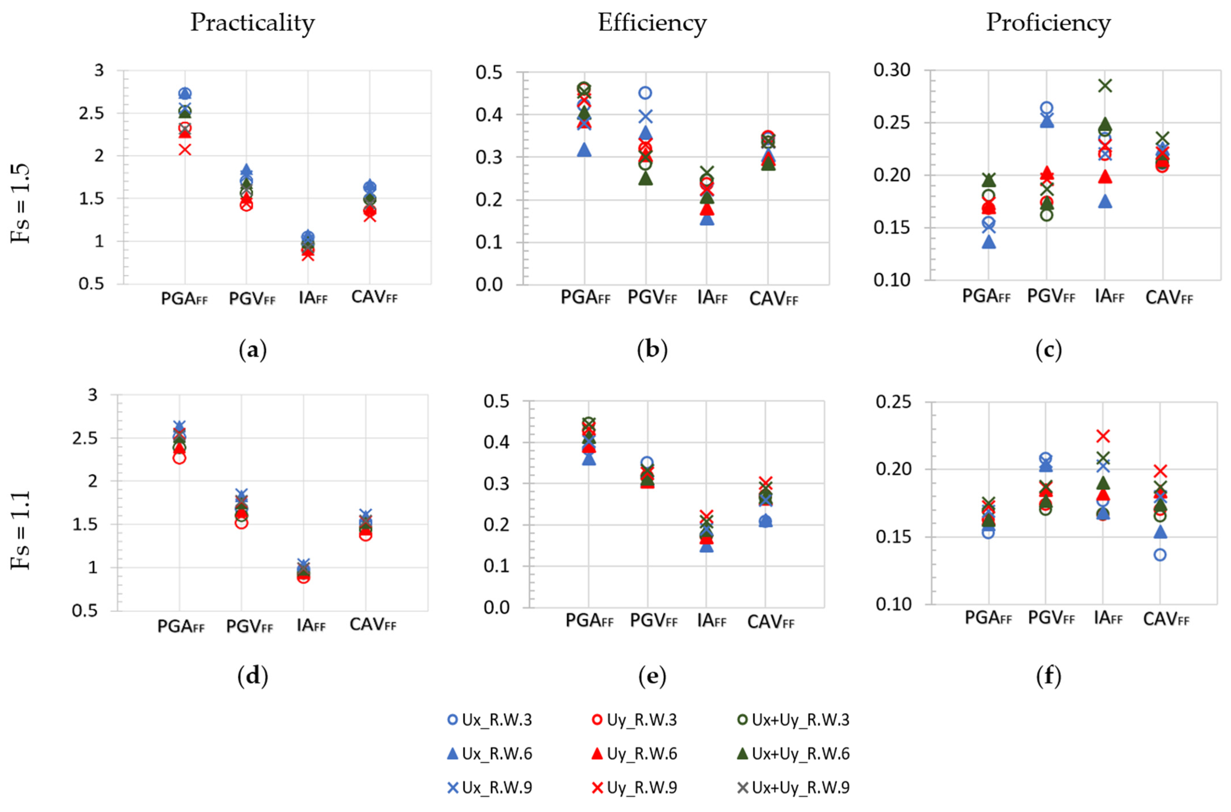
The seismic intensity was expressed by means of intensity measures (IM), which characterize the ground motion while showing a good correlation with the induced damage. Utilizing the outcomes of the dynamic analyses, the ln(IM)−ln(DI) dispersion plots were generated. Subsequently, the linear regression expressions were calculated in order to simulate the relationship between the different seismic intensity measures (independent variables) and the damage indices in terms of horizontal displacement of the base of the wall and vertical displacement of the backfill material (dependent variables). In addition, the approach of combined criteria was investigated, to estimate fragility due to the most critical damage mechanism. To derive the envelope fragility curves, new dispersion plots were generated utilizing both the outcomes of Ux and Uy as dependent variables. Specifically, the computed values of permanent horizontal displacements of the wall base were plotted together with the computed values of permanent vertical displacements of the backfill, versus the corresponding intensity measures. This resulted in the generation of linear regression expressions, accounting for both damage indices. The intensity measures selected for evaluation were the free field peak ground acceleration (PGAFF), as the most commonly used measure for describing ground motion, the free field peak ground velocity (PGVFF), and two parameters related to the energy content of the ground motion, namely the free field Arias intensity (IAFF), and the free field cumulative absolute velocity (CAVFF). The evaluation of the intensity measures was performed based on the criteria of practicality, efficiency, and proficiency [13]. Efficiency expresses the degree of dispersion of the structure’s response with respect to seismic intensity, and it is evaluated by the lognormal standard deviation of seismic demand (βD) or by the coefficient of determination (R2). Practicality expresses whether the intensity measure is directly correlated with the damage, evaluated by the slope of the linear relationship that describes the evolution of damage with the increasing seismic intensity. Proficiency is defined as the ratio of efficiency to practicality, expressing the composite result of the two criteria. A lower value of the ratio of lognormal standard deviation to the slope of the linear relationship indicates a more proficient intensity measure.
After defining the damage states and selecting the optimal seismic intensity measures, we proceeded to the calculation of probabilities of exceeding the three predefined damage states. This was achieved by applying the lognormal cumulative distribution function:
where is the probability of exceeding a damage state for a given level of seismic intensity, which is determined by the seismic intensity measure , is the standard cumulative probability function, is the median threshold value of the intensity measure required to cause the ith damage state, and is the total lognormal standard deviation. For the estimation of the total lognormal standard deviation, three different sources of uncertainty were taken into account, associated with the definition of damage states , the capacity of the element ), and the seismic input motion ), as described by Equation (5):
Finally, fragility curves were proposed. Concerning the approach of combined criteria, the envelope fragility curves were generated as the composite result of two sets of fragility curves, i.e., a set adopting the limit state values of the Ux criterion, and a set adopting the limit state values of the Uy criterion. The comprehensive assessment of the results indicated the impact of initial conditions and wall dimensions on the seismic fragility of typical cantilever retaining walls, as well as the most critical between the failure mechanisms under investigation.
3. Results
In this section, the results derived from the aforementioned methodology are presented with reference to the validation of the soil FE model, the estimation of the models’ fundamental frequencies, the evaluation of the intensity measures, and the estimation of the fragility parameters required to generate the fragility curves.
3.1. Validation of the Finite Element Soil Model
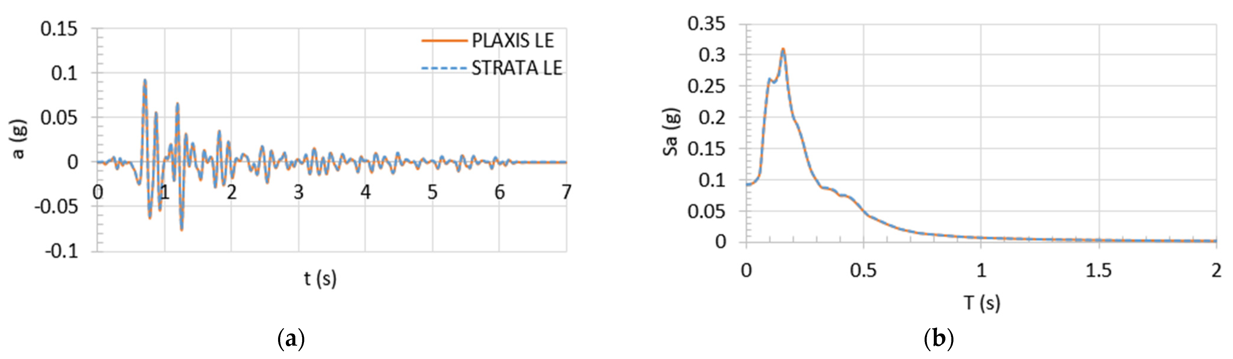
In order to calibrate the soil model and verify the validity of the FE seismic analyses results, the response of a 1D soil column created in PLAXIS was compared with the results, obtained from the 1D site response analysis software STRATA [29]. Initially, a linear elastic analysis was performed in STRATA by applying the weaker seismic motion ATH4_L2 (PGA = 0.0275 g), since the soil response is almost linear in the range of very small strains. The results demonstrated the response at the soil surface, and the Fourier transfer function between the response at the soil surface and the input motion indicated the fundamental natural frequency of the soil column f1 = 7.6 Hz and the second one f2 = 19 Hz. Thereafter, adopting the linear elastic constitutive model in PLAXIS, a 1D soil response analysis was performed, using 5% Rayleigh damping at frequencies 7.6 and 19 Hz. Figure 5 and Figure 6 depict that both analyses yield the same results of acceleration time histories and response spectra at the ground surface, as well as the transfer functions which also show a good convergence.
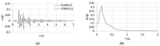
Figure 5.
Comparative representation of the results of the 1D linear elastic analyses performed by PLAXIS and STRATA, by applying the seismic motion ATH4_L2 (a) Acceleration time histories at the ground surface; (b) Acceleration response spectra at the ground surface.
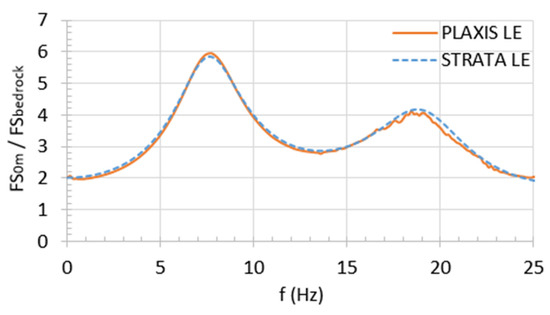
Figure 6.
Comparative representation of transfer function results derived from the 1D linear elastic analyses performed by PLAXIS and STRATA, by applying the seismic motion ATH4_L2.
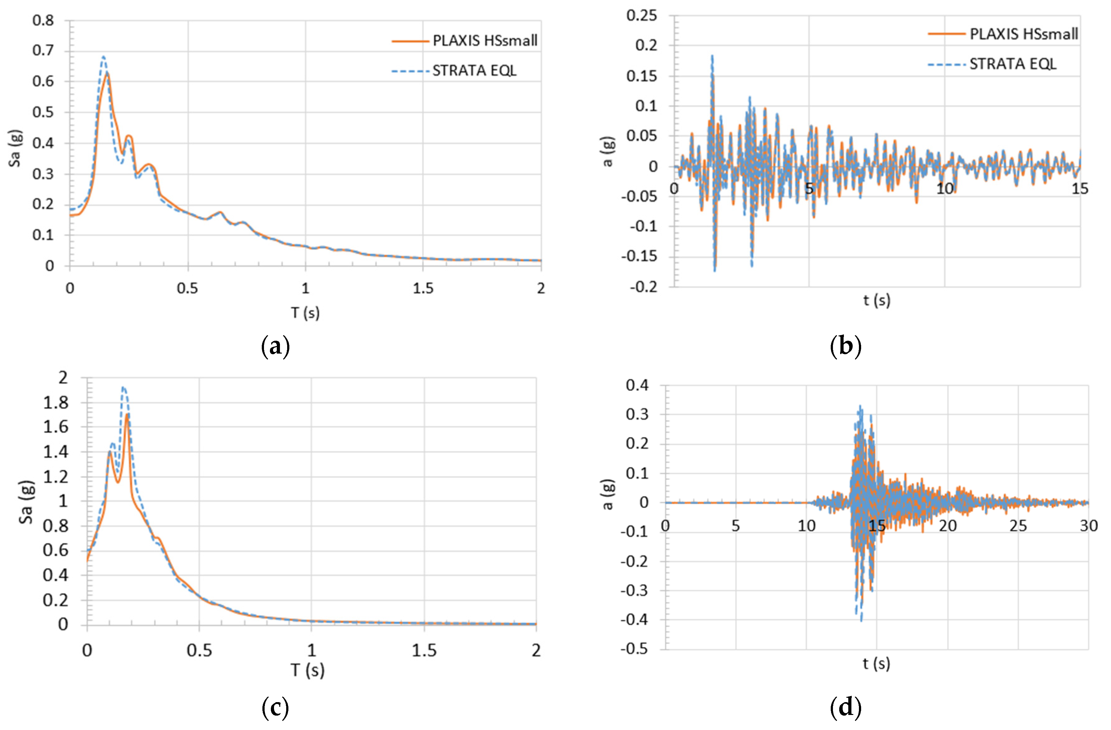
Subsequently, a comparative evaluation of soil response was carried out adopting the equivalent linear approach in STRATA and the non-linear HSsmall constitutive model in PLAXIS. To account for the hysteretic behavior of soil during the seismic loading in the equivalent linear analyses, shear modulus reduction and damping curves of Darendeli and Stokoe (2001) [30] were utilized. Figure 7 shows the response spectra and acceleration time histories at the ground surface, as obtained from the equivalent linear and non-linear analyses, by applying the input motions ZKRA_N (PGA = 0.0571 g), and VLSA_E (PGA = 0.1998 g). Since the deviations of the equivalent linear and non-linear approach depend on the degree of non-linearity of the soil, it is concluded that the PLAXIS 1D-wave propagation results show satisfactory convergence with those of STRATA, and therefore the validity of the soil simulation using the HSsmall constitutive model is verified.
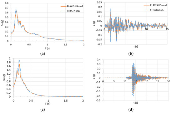
Figure 7.
Comparative representation of the results of the 1D non-linear analysis performed by PLAXIS and equivalent linear analysis performed by STRATA, by applying the seismic motion ZKRA_N (a) Acceleration response spectra at the ground surface; (b) Acceleration time histories at the ground surface; and by applying the seismic motion VLSA_E (c) Acceleration response spectra at the ground surface; (d) Acceleration time histories at the ground surface.
3.2. Estimation of Fundamental Frequencies
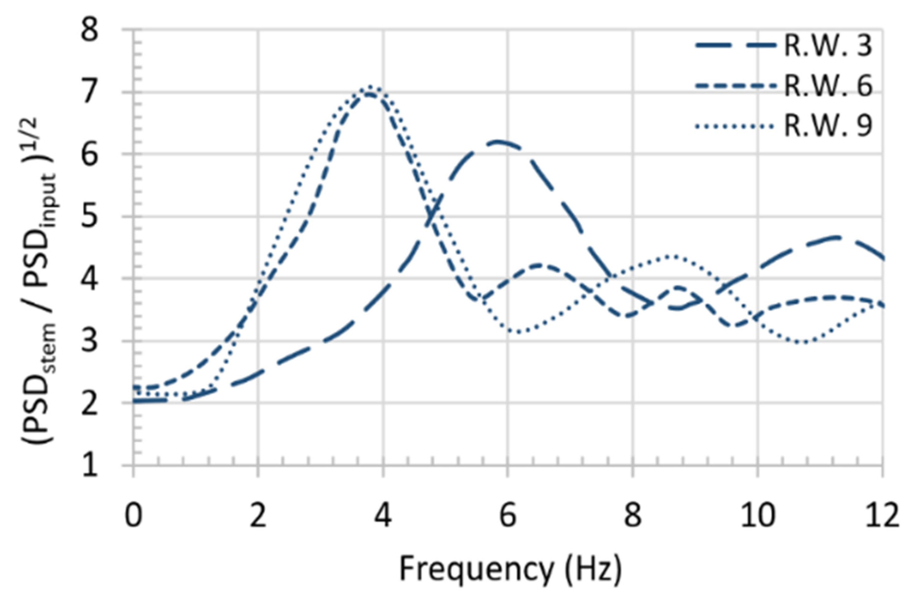
The root mean square of the power spectral density ratios, demonstrated the fundamental frequencies of the three retaining wall models, at 6 Hz for R.W.3, and around 4 Hz for the cases of R.W.6 and R.W.9. These results are depicted in Figure 8, for the input motion VSK_N scaled at a value of PGA equal to 0.1 g.
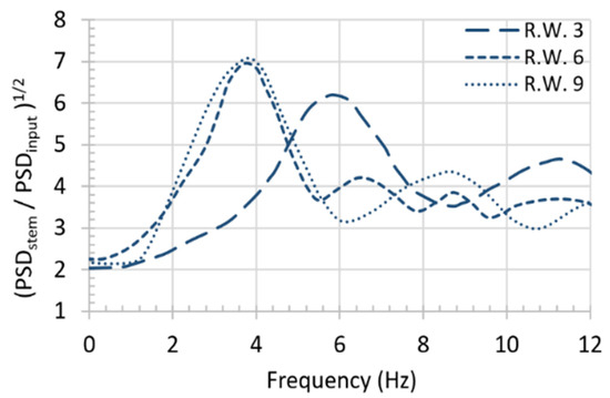
Figure 8.
Estimation of the root mean square of the power spectral density (PSD) ratios, utilizing the acceleration time histories generated by the 2D seismic analyses by applying the input motion VSK_N scaled at 0.1 g.
3.3. Evaluation of Intensity Measures
The parameters that characterize seismic intensity PGAFF, PGVFF, IAFF, and CAVFF were evaluated for their appropriateness in correlating with the induced damage, in terms of permanent horizontal displacement of the wall, permanent vertical displacement of the backfill, and the combination of the two damage criteria. The results of the investigation are expressed by rankings of practicality, efficiency, and proficiency, as presented in Table 7 and Table 8, for the two extreme cases of initial conditions, i.e., Fs = 1.5, and Fs = 1.1. Figure 9 also depicts the results plotted per criterion for each case of initial condition. It is observed that PGAFF is the most practical and proficient intensity measure, while in terms of efficiency it generally shows values of lognormal standard deviation < 0.46. In the case of IAFF, despite the maximum values of efficiency, the parameter shows the lowest degree of practicality and proficiency. CAVFF performs well for all three criteria, while for the PGVFF parameter, a generally satisfactory degree of efficiency, practicality, and proficiency is obtained.
Table 7.
Evaluation of intensity measures by practicality, efficiency, and proficiency criteria, in terms of permanent horizontal displacement of the wall base Ux, permanent vertical displacement of backfill Uy, and combining Ux + Uy, for the case of Fs = 1.5.
Table 8.
Evaluation of intensity measures by practicality, efficiency, and proficiency criteria, in terms of permanent horizontal displacement of the wall base Ux, permanent vertical displacement of backfill Uy, and combining Ux + Uy, for the case of Fs = 1.1.
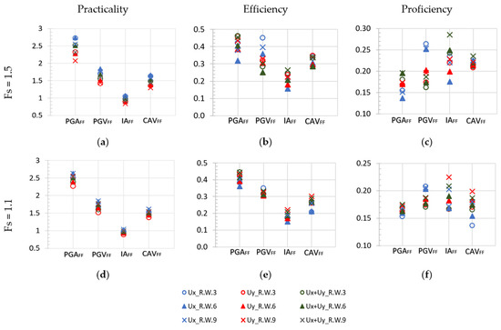
Figure 9.
Plotted rankings of practicality, efficiency, and proficiency criteria, in terms of permanent horizontal displacement of the wall base Ux, permanent vertical displacement of backfill Uy, and combining Ux + Uy (a–c) Regarding the case of Fs = 1.5 initial condition; (d–f) Regarding the case of Fs = 1.1 initial condition.
3.4. Fragility Function Parameters
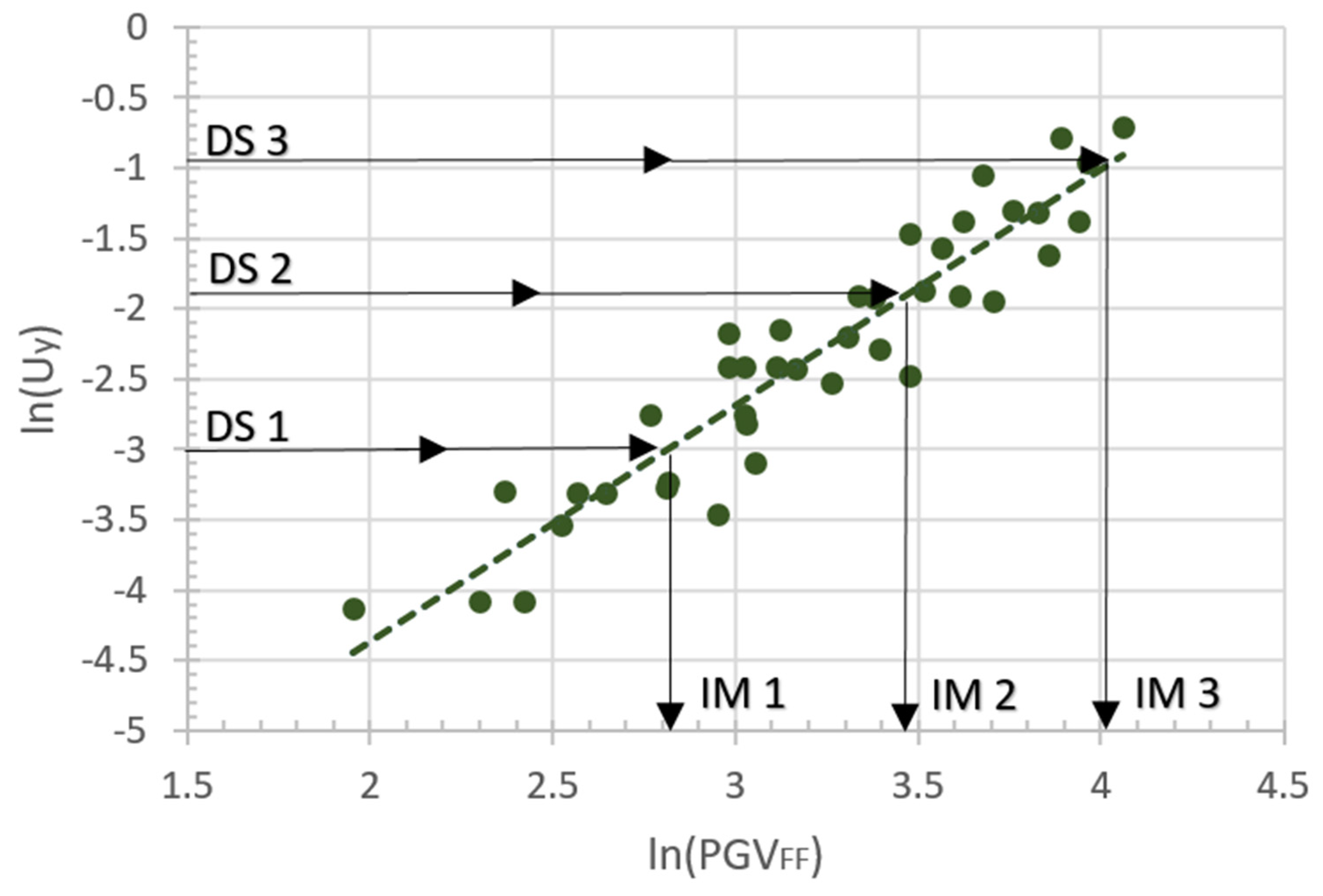
The implementation of the lognormal cumulative distribution function requires the estimation of the median threshold values for the three damage states, as well as the total lognormal standard deviation βtot. The median threshold values , were estimated for each damage state by the plots ln(IM) − ln(DI) that describe the evolution of damage with the increasing ground motion intensity. In Table 9, the values of and βtot are indicatively presented for the three cases of Fs = 1.5, 1.3, and 1.1, concerning the intensity measure PGAFF and the three damage indices, while Table A1, Table A2, Table A3, Table A4 and Table A5 in Appendix A include the fragility function parameters regarding all five initial conditions, in terms of PGAFF, PGVFF, and CAVFF, and Ux, Uy, and Ux + Uy. Figure 10 shows the case of R.W.6 for Fs = 1.2, considering the permanent vertical displacement of the backfill as damage index and the free field PGV as intensity measure. It should be noted that in cases where the calculated displacements were not sufficient to cause extensive damage, the linear relationship was extrapolated [13]. The uncertainties associated with the damage states can be addressed utilizing the maximum likelihood method, as presented in the work of Karakas et al. (2022) [31]. In this work, the values of the uncertainties and were set equal to 0.4 and 0.3 according to HAZUS (2004) [8]. The coefficient of uncertainty that expresses the deviation of the structure’s response at each intensity level due to the different input motions (, was calculated as the root mean square error of the differences between the damage index values predicted by the linear regression line, and the observed values that resulted from the dynamic analyses.
Table 9.
Fragility function parameters for the cases of Fs = 1.5, 1.3, and 1.1, for the IM PGAFF.

Figure 10.
Linear regression line of the dispersion plot, expressing damage evolution in terms of permanent vertical displacement of the backfill, with increasing ground motion intensity in terms of free field PGV; case of R.W. 6 for initial condition Fs = 1.2.
Regarding the investigation of combined criteria, the comparative assessment of fragility curves generated by adopting (a) the limit values of Ux criterion, and (b) the limit values of Uy criterion indicated that higher probabilities of damage arise from the second case, with the exception of R.W.3 for DS3. This is a reasonable conclusion due to the fact that the vertical displacement criterion requires generally lower limit state values than the horizontal displacement criterion. However, this statement does not apply to the case of R.W.3 for DS3, where the Ux threshold required to cause extensive damage (0.30 m) is lower than the corresponding Uy threshold (0.40 m). Hence, accounting for this exclusion, it is concluded that the envelope fragility curves are derived by adopting the limit values of the Uy criterion, indicating that the permanent vertical displacement of the backfill is a more critical mechanism for seismic induced damage on cantilever retaining walls.
3.5. Fragility Curves
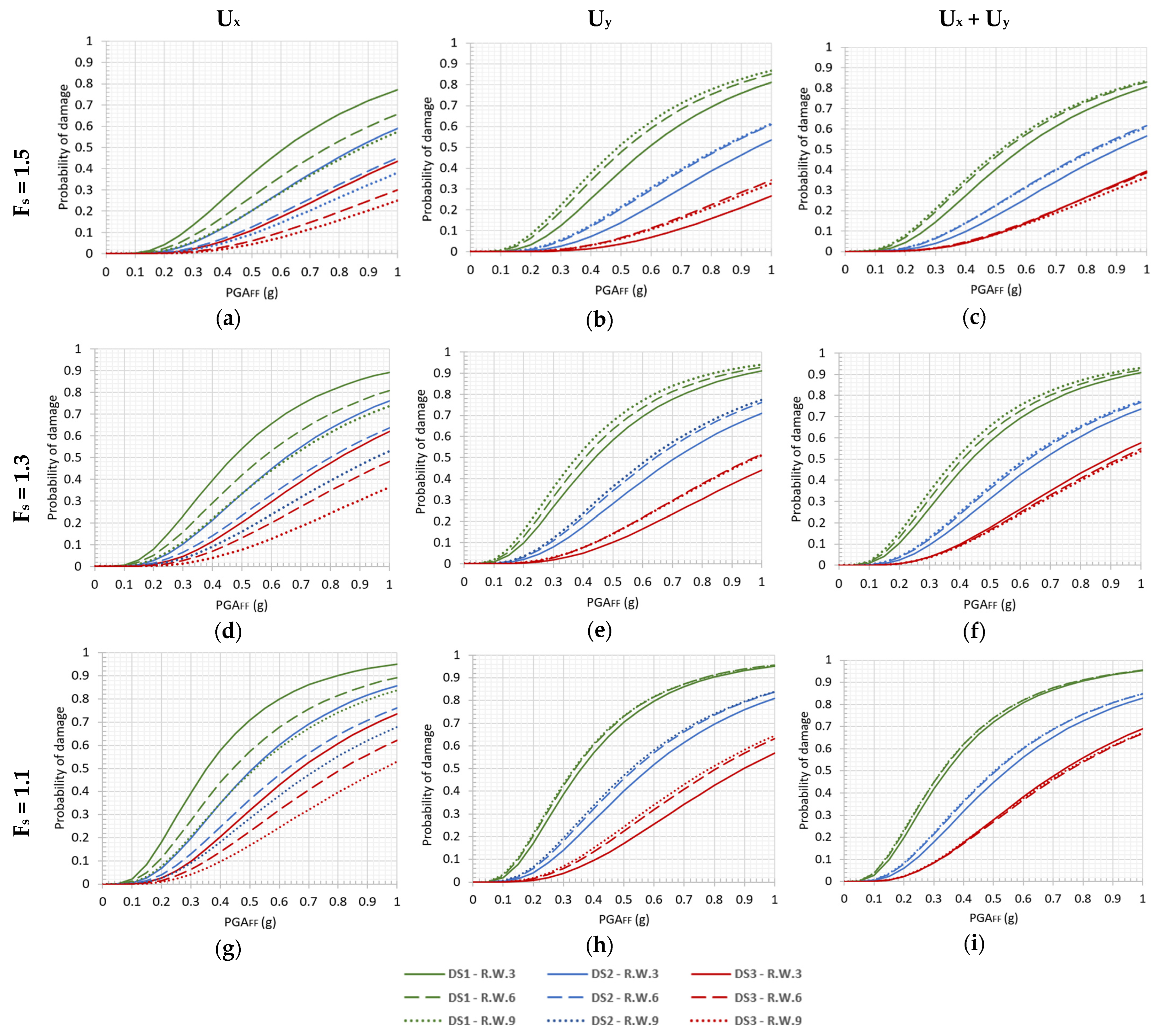
Based on the implementation of the computed fragility curves parameters, IMmi, concerning the three damage states, and βtot (Table 9, and Table A1, Table A2, Table A3, Table A4 and Table A5 in Appendix A) to the lognormal cumulative distribution function (Equation (4)), the probabilities of exceeding each damage state for a given level of seismic intensity were calculated. Hence, the corresponding fragility curves for the three models R.W.3, R.W.6, and R.W.9 were proposed, referring to the five cases of initial conditions defined by the different values of global Fs. Figure 11 illustrates the fragility curves for Fs = 1.5, 1.3, and 1.1, in terms of PGAFF − DIs, while the fragility curves regarding all five initial conditions, in terms of PGAFF, PGVFF, and CAVFF, and Ux, Uy, and Ux + Uy, are illustrated on Figure A1, Figure A2, Figure A3, Figure A4 and Figure A5, in Appendix B.
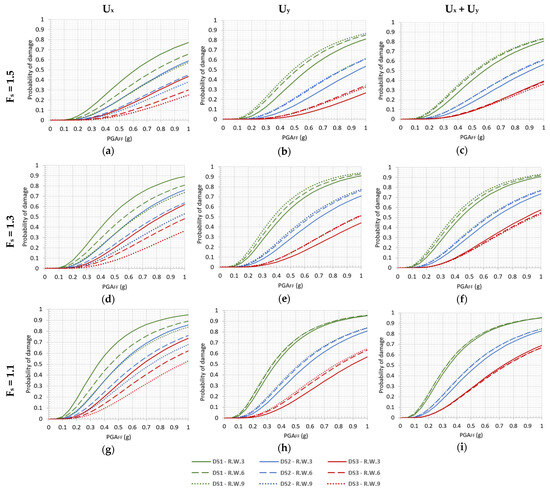
Figure 11.
Fragility curves for cantilever retaining walls R.W.3, R.W.6, R.W.9, in terms of PGAFF − DI, regarding the cases of initial conditions Fs = 1.5 (a–c); Fs = 1.3 (d–f); and Fs = 1.1 (g–i).
The proposed fragility curves in terms of permanent vertical displacement of the backfill (Uy) denote that retaining walls R.W.6 and R.W.9 show approximately the same degree of fragility at each damage state, with divergence in damage probability lower than 5%. On the contrary, reduced fragility levels are presented for R.W.3, showing about 8–20% lower probabilities of damage than R.W.6. This difference between R.W.3 and the higher walls seems to be decaying with the decrease of Fs; while shorter deviation is generally observed in the cases of minor damage (DS1). The fragility curves proposed by adopting the combined criteria (Ux + Uy) denote overall similar remarks with the ones proposed by adopting Uy criterion, with the exception of extensive damage state (DS3) where all three walls show almost the same degree of fragility, regardless of their height. On the other hand, fragility curves calculated considering the permanent horizontal displacement of the base (Ux) as a damage index illustrate a different pattern on damage probability regarding the three models R.W.3, R.W.6, and R.W.9. Particularly, higher probabilities of damage are presented for walls of lower height. This pattern is retrieved from the definition of limit states as a percentage of the wall height. Therefore, R.W.3 requires lower values of horizontal displacement to exceed each damage state (0.06 m, 0.15 m, 0.30 m), as opposed to the corresponding values for R.W.6 (0.12 m, 0.30 m, 0.60 m), and R.W.9 (0.18 m, 0.45 m, 0.90 m). Considering that the horizontal displacement of the base represents the failure mechanism of sliding, whereas the vertical displacement of the backfill might result from the composite effect of sliding and rotation, it can be concluded that Uy is a more critical damage index than Ux.
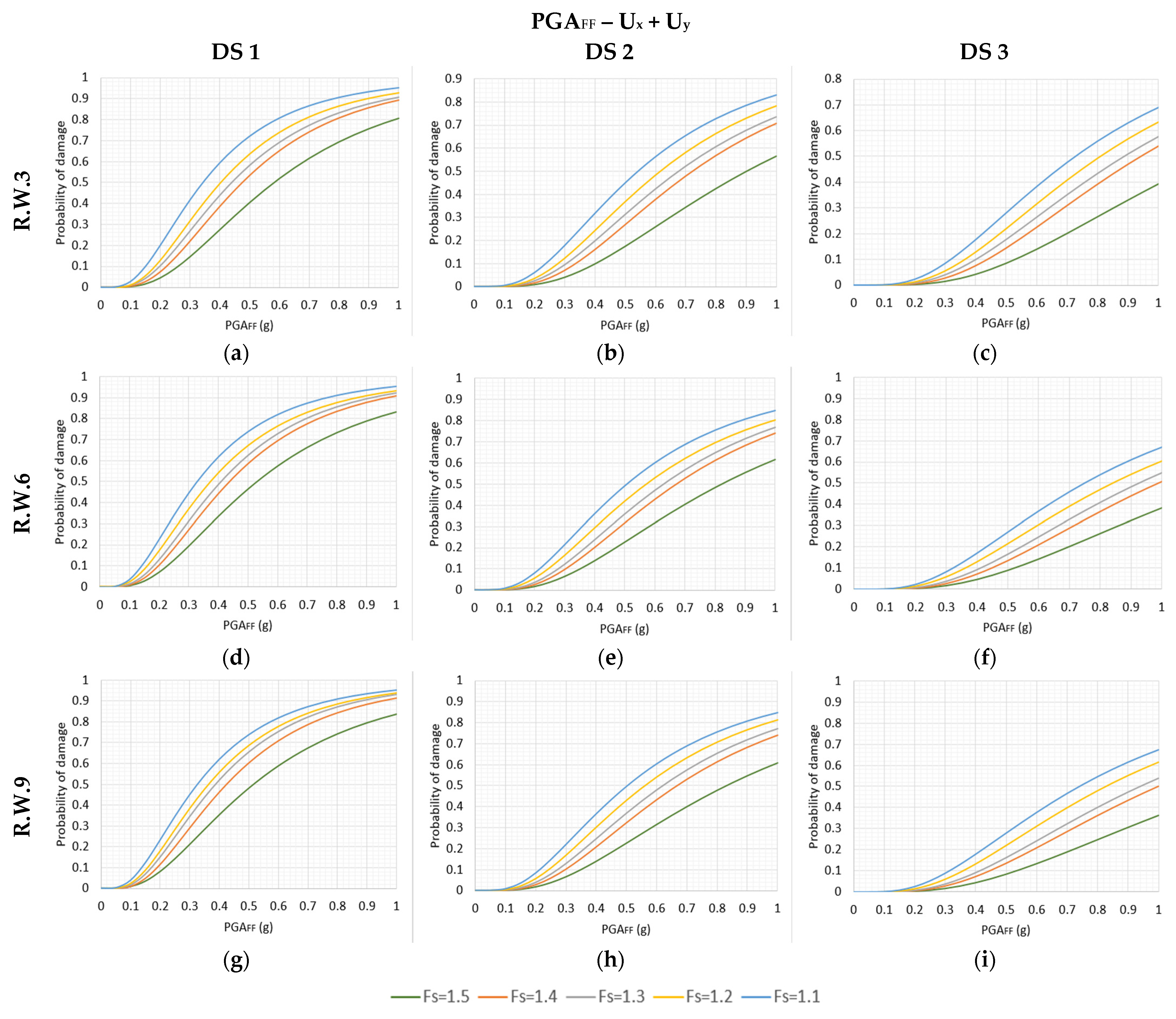
For the comparative assessment of fragility curves referring to different initial conditions, Figure A6, Figure A7, Figure A8, Figure A9, Figure A10, Figure A11, Figure A12, Figure A13 and Figure A14, in Appendix C are presented. Herein, Figure 12 indicatively illustrates the cases of PGAFF − Ux + Uy. Each figure corresponds to a different case of IM−DI, while each plot refers to an individual soil-wall model at a certain damage state. As expected, lower values of Fs result to higher values of damage probability. In cases where the presence of water table is considered, i.e., Fs = 1.1, 1.2, 1.3, 1.4, there is a relatively small change in the degree of fragility between two sequencing initial conditions. On the contrary, fragility curves corresponding to dry initial conditions, i.e., Fs = 1.5, show considerably lower probabilities of damage than the following curves of Fs = 1.4. In the case of R.W.3, DS2 for PGAFF = 0.5 g, the estimated probabilities of damage for Fs = 1.1, 1.2, 1.3, and 1.4 are equal to 45%, 37%, 32%, and 27%, respectively; while for Fs = 1.5 the probability of damage drops to 17%, demonstrating that there is no proportionality in the degradation of fragility curves.
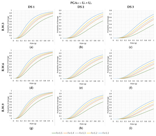
Figure 12.
Fragility curves for different initial conditions regarding the value of Fs = 1.1–1.5, in terms of PGAFF − Ux + Uy, for the cases of (a) R.W.3 − DS1; (b) R.W.3 − DS2; (c) R.W.3 − DS3; (d) R.W.6 − DS1; (e) R.W.6 − DS2; (f) R.W.6 − DS3; (g) R.W.9 − DS1; (h) R.W.9 − DS2; (i) R.W.9 − DS3.
4. Discussion
In this study, novel fragility curves for typical cantilever retaining walls have been developed, with the aim of investigating the impact of initial conditions on seismic fragility. Three retaining wall models of the same typology but with different heights were simulated in order to compute their seismic response, considering dry conditions and also the presence of water table at four different levels, leading to five discrete values of global safety factor ranging from 1.1 to 1.5. Damage probability was determined in terms of permanent horizontal displacement of wall base, permanent vertical displacement of backfill, and utilizing the outcomes of both horizontal and vertical displacements, with respect to increasing seismic intensity.
At an early stage of the investigation, the estimation of fundamental frequencies of the three soil-wall models resulted in the same value of f1 = 4 Hz, for R.W.6 and R.W.9, indicating a potential similar dynamic response for the two models. This was later verified by the fragility curves proposed in terms of Uy and Ux + Uy, with the two walls showing approximately the same degree of fragility. Additionally, R.W.3 showed lower probabilities of damage, demonstrating that with a decrease in height, the induced seismic deformation reduces. On the other hand, a reversed pattern was observed in the case of fragility curves proposed in terms of Ux, resulting from the definition of limit state displacements as a percentage of wall height. Consequently, it is evident that the selection of the damage index, as well as the definition of damage states, plays a significant role on the formulation of fragility curves.
To calculate an envelope curve representative of the most unfavorable damage scenario at each intensity level, the approach of combining two damage criteria was implemented. The results denoted the vertical displacement of backfill as the critical damage index, leading to higher probabilities of damage compared to horizontal displacement, with the exception of only one case (R.W.3 − DS3). Taking into account that the horizontal displacement of the wall base is correlated with the failure mechanism of sliding, while the vertical displacement of backfill might result from the contribution of both sliding and overturning, the aforementioned remark can be regarded reasonable.
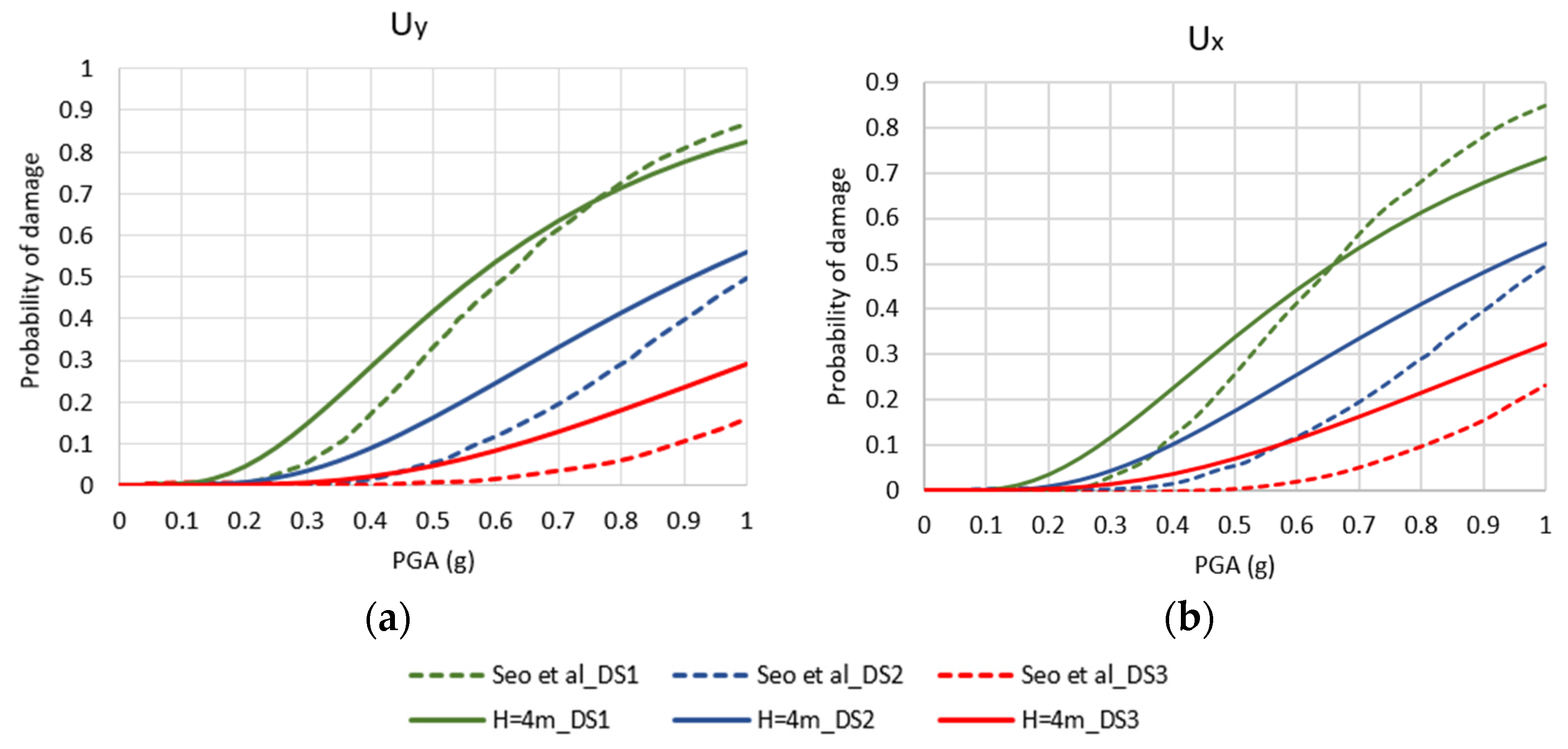
In order to validate the proposed fragility curves, a comparative assessment with existing curves from the literature was made. The research that has been carried out so far concerns different typologies of retaining walls and soil properties, leading to variable results. Hence, the proposed fragility curves by Seo et al. [14] regarding a 4m height cantilever retaining wall model with cohesionless soil corresponding to site category S2 of the South Korean classification system, were chosen for this comparison. Figure 13, depicts the fragility curves by Seo et al. (dashed), along with the newly proposed curves (continuous) that were retrieved after interpolation between the R.W.3 and R.W.6 curves for Fs = 1.5, in terms of PGAFF − Uy, and PGAFF − Ux. In the case of Uy, the two sets of fragility curves corresponding to minor damage show a maximum divergence in damage probability around 10%, for PGA = 0.3–0.4 g. In the case of Ux, the sets of curves corresponding to DS1 show a maximum divergence around 12%, for the larger PGA values. For both damage indices, the proposed curves of this work illustrate 10–13% higher damage probabilities for moderate PGA values in DS2, whereas the same divergence is observed in DS3 for larger PGA values. The lower damage probabilities concerning the curves from literature, might be attributed to the presence of a shear key at the base of the retaining wall model, resulting in a higher sliding resistance.
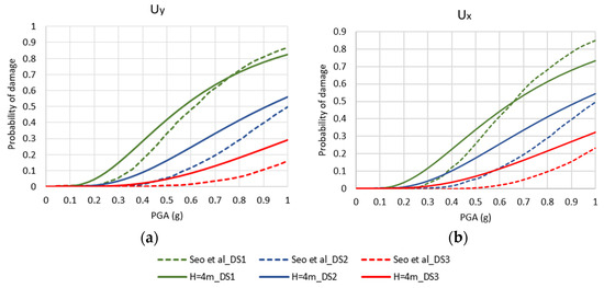
Figure 13.
Comparative representation of the fragility curves by Seo et al. [14] and the proposed curves of this study, in terms of (a) PGAFF − Uy; (b) PGAFF − Ux.
The comparative representation of fragility curves derived for different values of safety factor demonstrated the effect of initial conditions to the degree of seismic fragility. In cases of heavy rainfall or retaining walls with malfunctioning/insufficient drainage, the implementation of fragility curves corresponding to Fs = 1.1 would be recommended in order to cover all intermediate initial conditions. In cases of dry conditions, fragility curves corresponding to Fs = 1.5 shall be implemented. Future research could further examine in what way factors other than the level of water table will affect the degree of fragility, assuming the same initial conditions of Fs = 1.1–1.5. The proposed fragility curves constitute a reliable tool that can be utilized in conjunction with seismic hazard analysis results in seismic risk assessment. The results of this investigation were derived concerning cohesionless soil materials, and typical geometries of cantilever retaining walls. For retaining structures of different typology, relevant fragility curves should be considered or developed. Regarding pore water pressure, the assumption of hydrostatic conditions has been made. For a more realistic simulation of water conditions, groundwater flow could be taken into account in future research work.
Author Contributions
Conceptualization, E.-I.K., D.S. and N.K.; methodology, E.-I.K. and N.K.; software, E.-I.K.; validation, E.-I.K. and D.S.; investigation, E.-I.K., D.S. and N.K.; resources, I.D.; data curation, E.-I.K., D.S. and N.K.; writing—original draft preparation, E.-I.K.; writing—review and editing, D.S. and N.K; supervision, N.K. All authors have read and agreed to the published version of the manuscript.
Funding
We acknowledge the support of this work by the project “Risk and Resilience Assessment Center–Prefecture of East Macedonia and Thrace-Greece” (MIS 5047293), which is implemented under the action “Reinforcement of the Research and Innovation Infrastructure”, funded by the operational program “Competitiveness, Entrepreneurship and Innovation” (NSRF 2014–2020), and co-financed by Greece and the European Union (European Regional Development Fund).
Data Availability Statement
Data are contained within the article.
Conflicts of Interest
The authors declare no conflict of interest.
Appendix A
Table A1, Table A2, Table A3, Table A4 and Table A5 provide the fragility function parameters regarding all five initial conditions of Fs = 1.5, 1.4, 1.3, 1.2, and 1.1, in terms of intensity measures PGAFF, PGVFF, and CAVFF and damage indices Ux, Uy, and Ux + Uy.
Table A1.
Fragility function parameters for the case of Fs = 1.5.
Table A1.
Fragility function parameters for the case of Fs = 1.5.
| Fs = 1.5 | PGAFF (g) | PGVFF (cm/s) | CAVFF (cm/s) | |||||||
|---|---|---|---|---|---|---|---|---|---|---|
| R.W.3 | R.W.6 | R.W.9 | R.W.3 | R.W.6 | R.W.9 | R.W.3 | R.W.6 | R.W.9 | ||
| Ux | DS1 = 2% H | 0.6157 | 0.7606 | 0.8814 | 32.3536 | 43.1532 | 53.416 | 1518.491 | 2125.69 | 2707.35 |
| DS2 = 5% H | 0.8623 | 1.0883 | 1.2297 | 55.3547 | 72.6084 | 86.599 | 2664.446 | 3800.48 | 4654.50 | |
| DS3 = 10% H | 1.1126 | 1.4271 | 1.5821 | 83.097 | 107.6291 | 124.811 | 4076.93 | 5898.29 | 7012.81 | |
| 0.654 | 0.6791 | 0.6802 | 0.6725 | 0.5939 | 0.5751 | 0.6069 | 0.6088 | 0.6012 | ||
| Uy | DS1 = 0.05 m | 0.5921 | 0.5184 | 0.4895 | 30.5131 | 24.6776 | 22.7852 | 1428.17 | 1140.607 | 1042.22 |
| DS2 = 0.15 m | 0.9496 | 0.8393 | 0.8316 | 66.0500 | 50.9801 | 48.7478 | 3209.64 | 2520.741 | 2433.45 | |
| DS3 = 0.40 m | 1.4480 | 1.2906 | 1.3348 | 131.6141 | 97.4354 | 96.1269 | 6613.49 | 5116.797 | 5188.05 | |
| 0.5928 | 0.6315 | 0.6434 | 0.6321 | 0.5862 | 0.5593 | 0.5858 | 0.5815 | 0.5759 | ||
| Ux + Uy | DS1 = 0.05 m | 0.5832 | 0.5305 | 0.5168 | 29.7201 | 25.5531 | 24.6296 | 1389.64 | 1184.26 | 1136.40 |
| DS2 = 0.15 m | 0.9015 | 0.8218 | 0.8307 | 59.9842 | 49.1258 | 48.8827 | 2900.37 | 2432.02 | 2441.86 | |
| DS3 = 0.40 m (0.3 m) * | 1.1866 | 1.2147 | 1.2689 | 93.4247 | 88.0525 | 90.1441 | 4613.89 | 4623.59 | 4833.86 | |
| 0.6281 | 0.6623 | 0.6752 | 0.6573 | 0.5989 | 0.5828 | 0.6022 | 0.6032 | 0.6034 | ||
* Limit value of DS3 for the case of R.W.3.
Table A2.
Fragility function parameters for the case of Fs = 1.4.
Table A2.
Fragility function parameters for the case of Fs = 1.4.
| Fs = 1.4 | PGAFF (g) | PGVFF (cm/s) | CAVFF (cm/s) | |||||||
|---|---|---|---|---|---|---|---|---|---|---|
| R.W.3 | R.W.6 | R.W.9 | R.W.3 | R.W.6 | R.W.9 | R.W.3 | R.W.6 | R.W.9 | ||
| Ux | DS1 = 2% H | 0.5026 | 0.6129 | 0.7211 | 25.1296 | 33.6937 | 42.4850 | 1185.82 | 1665.457 | 2184.628 |
| DS2 = 5% H | 0.6952 | 0.8568 | 1.0234 | 41.9035 | 55.4081 | 70.8132 | 2094.93 | 2958.293 | 3954.065 | |
| DS3 = 10% H | 0.8886 | 1.1041 | 1.3338 | 61.6929 | 80.7217 | 104.222 | 3222.06 | 4568.636 | 6193.854 | |
| 0.6044 | 0.6293 | 0.6343 | 0.66 | 0.6022 | 0.586 | 0.5936 | 0.5864 | 0.5786 | ||
| Uy | DS1 = 0.05 m | 0.4795 | 0.4278 | 0.4049 | 23.3239 | 19.7387 | 18.3320 | 1092.284 | 899.90 | 825.12 |
| DS2 = 0.15 m | 0.7568 | 0.6830 | 0.6631 | 48.1952 | 39.6561 | 37.5181 | 2439.71 | 1999.71 | 1886.05 | |
| DS3 = 0.40 m | 1.1372 | 1.0370 | 1.0300 | 92.1325 | 73.9295 | 71.1092 | 4999.468 | 4079.05 | 3945.43 | |
| 0.5753 | 0.6038 | 0.61 | 0.6274 | 0.5881 | 0.5686 | 0.5721 | 0.5657 | 0.5564 | ||
| Ux + Uy | DS1 = 0.05 m | 0.4750 | 0.4369 | 0.4245 | 22.9807 | 20.3812 | 19.6257 | 1074.08 | 932.69 | 891.44 |
| DS2 = 0.15 m | 0.7229 | 0.6732 | 0.6682 | 44.6704 | 38.7713 | 37.9846 | 2246.74 | 1954.08 | 1915.08 | |
| DS3 = 0.40 m (0.3 m) * | 0.9422 | 0.9903 | 1.0018 | 67.9425 | 68.8411 | 68.4928 | 3579.13 | 3781.93 | 3790.34 | |
| 0.595 | 0.6206 | 0.6302 | 0.6486 | 0.60 | 0.59 | 0.5883 | 0.5804 | 0.576 | ||
* Limit value of DS3 for the case of R.W.3.
Table A3.
Fragility function parameters for the case of Fs = 1.3.
Table A3.
Fragility function parameters for the case of Fs = 1.3.
| Fs = 1.3 | PGAFF (g) | PGVFF (cm/s) | CAVFF (cm/s) | |||||||
|---|---|---|---|---|---|---|---|---|---|---|
| R.W.3 | R.W.6 | R.W.9 | R.W.3 | R.W.6 | R.W.9 | R.W.3 | R.W.6 | R.W.9 | ||
| Ux | DS1 = 2% H | 0.4693 | 0.5701 | 0.6610 | 22.5841 | 30.1715 | 37.4722 | 1053.48 | 1467.58 | 1864.34 |
| DS2 = 5% H | 0.6496 | 0.7982 | 0.9526 | 37.4521 | 49.3309 | 63.9797 | 1850.35 | 2593.36 | 3413.58 | |
| DS3 = 10% H | 0.8307 | 1.0296 | 1.2561 | 54.9103 | 71.5552 | 95.8949 | 2833.42 | 3989.40 | 5394.14 | |
| 0.609 | 0.6439 | 0.6497 | 0.6479 | 0.5945 | 0.6107 | 0.5794 | 0.5823 | 0.5681 | ||
| Uy | DS1 = 0.05 m | 0.4395 | 0.4047 | 0.3767 | 20.5171 | 18.2550 | 16.4840 | 942.97 | 822.66 | 738.69 |
| DS2 = 0.15 m | 0.7115 | 0.6432 | 0.6243 | 42.4034 | 36.0423 | 34.4060 | 2143.86 | 1794.78 | 1689.12 | |
| DS3 = 0.40 m | 1.0939 | 0.9727 | 0.9803 | 81.0744 | 66.1562 | 66.3659 | 4463.28 | 3601.48 | 3534.67 | |
| 0.6127 | 0.6198 | 0.6265 | 0.6087 | 0.5869 | 0.5912 | 0.5763 | 0.5657 | 0.5515 | ||
| Ux + Uy | DS1 = 0.05 m | 0.4397 | 0.4093 | 0.3872 | 20.4644 | 18.5798 | 17.1428 | 942.10 | 838.28 | 770.95 |
| DS2 = 0.15 m | 0.6766 | 0.6300 | 0.6191 | 39.6285 | 34.9430 | 34.0207 | 1976.96 | 1736.26 | 1669.75 | |
| DS3 = 0.40 m (0.3 m) * | 0.888 | 0.9260 | 0.9414 | 60.13 | 61.4141 | 62.7325 | 3155.68 | 3326.13 | 3328.83 | |
| 0.6184 | 0.6348 | 0.6409 | 0.634 | 0.5941 | 0.6039 | 0.5851 | 0.5772 | 0.5629 | ||
* Limit value of DS3 for the case of R.W.3.
Table A4.
Fragility function parameters for the case of Fs = 1.2.
Table A4.
Fragility function parameters for the case of Fs = 1.2.
| Fs = 1.2 | PGAFF (g) | PGVFF (cm/s) | CAVFF (cm/s) | |||||||
|---|---|---|---|---|---|---|---|---|---|---|
| R.W.3 | R.W.6 | R.W.9 | R.W.3 | R.W.6 | R.W.9 | R.W.3 | R.W.6 | R.W.9 | ||
| Ux | DS1 = 2% H | 0.4193 | 0.5087 | 0.5869 | 19.0396 | 25.5276 | 31.3448 | 870.61 | 1209.09 | 1532.96 |
| DS2 = 5% H | 0.5872 | 0.7128 | 0.8273 | 31.8545 | 41.5207 | 51.3266 | 1544.27 | 2119.65 | 2712.24 | |
| DS3 = 10% H | 0.7576 | 0.9200 | 1.0727 | 47.0165 | 59.9891 | 74.5351 | 2382.36 | 3241.12 | 4176.20 | |
| 0.6171 | 0.6607 | 0.6591 | 0.6297 | 0.5931 | 0.5877 | 0.5615 | 0.575 | 0.574 | ||
| Uy | DS1 = 0.05 m | 0.4138 | 0.3786 | 0.3637 | 18.6337 | 16.6714 | 15.7620 | 852.11 | 741.20 | 693.78 |
| DS2 = 0.15 m | 0.6535 | 0.5962 | 0.5776 | 37.5950 | 32.0919 | 30.6399 | 1853.20 | 1571.14 | 1491.41 | |
| DS3 = 0.40 m | 0.9826 | 0.8943 | 0.8730 | 70.3526 | 57.5871 | 55.4641 | 3708.28 | 3072.67 | 2953.49 | |
| 0.6008 | 0.6441 | 0.6382 | 0.6169 | 0.5896 | 0.581 | 0.5561 | 0.5673 | 0.5638 | ||
| Ux + Uy | DS1 = 0.05 m | 0.4021 | 0.3732 | 0.3634 | 17.8484 | 16.3341 | 15.7456 | 811.00 | 723.19 | 692.24 |
| DS2 = 0.15 m | 0.6174 | 0.5725 | 0.5619 | 34.4210 | 30.2726 | 29.4416 | 1681.70 | 1471.07 | 1425.63 | |
| DS3 = 0.40 m (0.3 m) * | 0.8092 | 0.8389 | 0.8290 | 52.0929 | 52.5143 | 51.4782 | 2664.3 | 2772.99 | 2717.18 | |
| 0.6198 | 0.6588 | 0.8290 | 0.634 | 0.5986 | 0.5886 | 0.5707 | 0.5785 | 0.5732 | ||
* Limit value of DS3 for the case of R.W.3.
Table A5.
Fragility function parameters for the case of Fs = 1.1.
Table A5.
Fragility function parameters for the case of Fs = 1.1.
| Fs = 1.1 | PGAFF (g) | PGVFF (cm/s) | CAVFF (cm/s) | |||||||
|---|---|---|---|---|---|---|---|---|---|---|
| R.W.3 | R.W.6 | R.W.9 | R.W.3 | R.W.6 | R.W.9 | R.W.3 | R.W.6 | R.W.9 | ||
| Ux | DS1 = 2% H | 0.3541 | 0.4428 | 0.5181 | 17.5285 | 20.9055 | 26.1938 | 664.5898 | 961.29 | 1244.70 |
| DS2 = 5% H | 0.5104 | 0.6272 | 0.7334 | 30.2031 | 34.5115 | 42.9926 | 1214.915 | 1709.97 | 2199.65 | |
| DS3 = 10% H | 0.6729 | 0.8160 | 0.9539 | 45.5838 | 50.4254 | 62.5436 | 1917.5 | 2643.68 | 3383.94 | |
| 0.6296 | 0.6577 | 0.6695 | 0.6105 | 0.5924 | 0.5906 | 0.5412 | 0.5684 | 0.5662 | ||
| Uy | DS1 = 0.05 m | 0.3594 | 0.3390 | 0.3342 | 15.2181 | 14.1858 | 13.9660 | 681.658 | 615.79 | 604.98 |
| DS2 = 0.15 m | 0.5835 | 0.5366 | 0.5250 | 31.3723 | 27.5836 | 26.7082 | 1515.791 | 1321.42 | 1273.16 | |
| DS3 = 0.40 m | 0.8994 | 0.8085 | 0.7857 | 59.8476 | 49.9442 | 47.6461 | 3093.871 | 2612.75 | 2473.90 | |
| 0.6169 | 0.6346 | 0.6491 | 0.6037 | 0.5858 | 0.589 | 0.5429 | 0.5653 | 0.5668 | ||
| Ux + Uy | DS1 = 0.05 m | 0.3433 | 0.3276 | 0.3261 | 14.2198 | 13.5224 | 13.5081 | 631.57 | 582.65 | 581.79 |
| DS2 = 0.15 m | 0.5439 | 0.5073 | 0.503 | 28.2392 | 25.4251 | 25.1111 | 1349.58 | 1203.27 | 1185.77 | |
| DS3 = 0.40 m (0.3m) * | 0.7271 | 0.7495 | 0.7406 | 43.5355 | 44.6757 | 43.6785 | 2179.04 | 2299.05 | 2239.16 | |
| 0.642 | 0.6608 | 0.6683 | 0.6265 | 0.6054 | 0.60 | 0.5637 | 0.5838 | 0.5771 | ||
* Limit value of DS3 for the case of R.W.3.
Appendix B
We provide the proposed fragility curves for the three models R.W.3, R.W.6, and R.W.9, referring to the five cases of initial conditions of Fs = 1.5, 1.4, 1.3, 1.2, and 1.1, in terms of intensity measures PGAFF, PGVFF, and CAVFF, and damage indices Ux, Uy, and Ux + Uy.
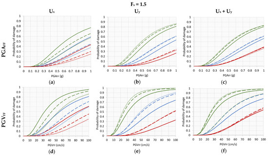
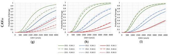
Figure A1.
Fragility curves for cantilever retaining walls R.W.3, R.W.6, R.W.9, regarding the case of initial condition Fs = 1.5, in terms of (a) PGAFF − Ux; (b) PGAFF − Uy; (c) PGAFF − Ux + Uy; (d) PGVFF − Ux; (e) PGVFF − Uy; (f) PGVFF − Ux + Uy; (g) CAVFF − Ux; (h) CAVFF − Uy; (i) CAVFF − Ux + Uy.
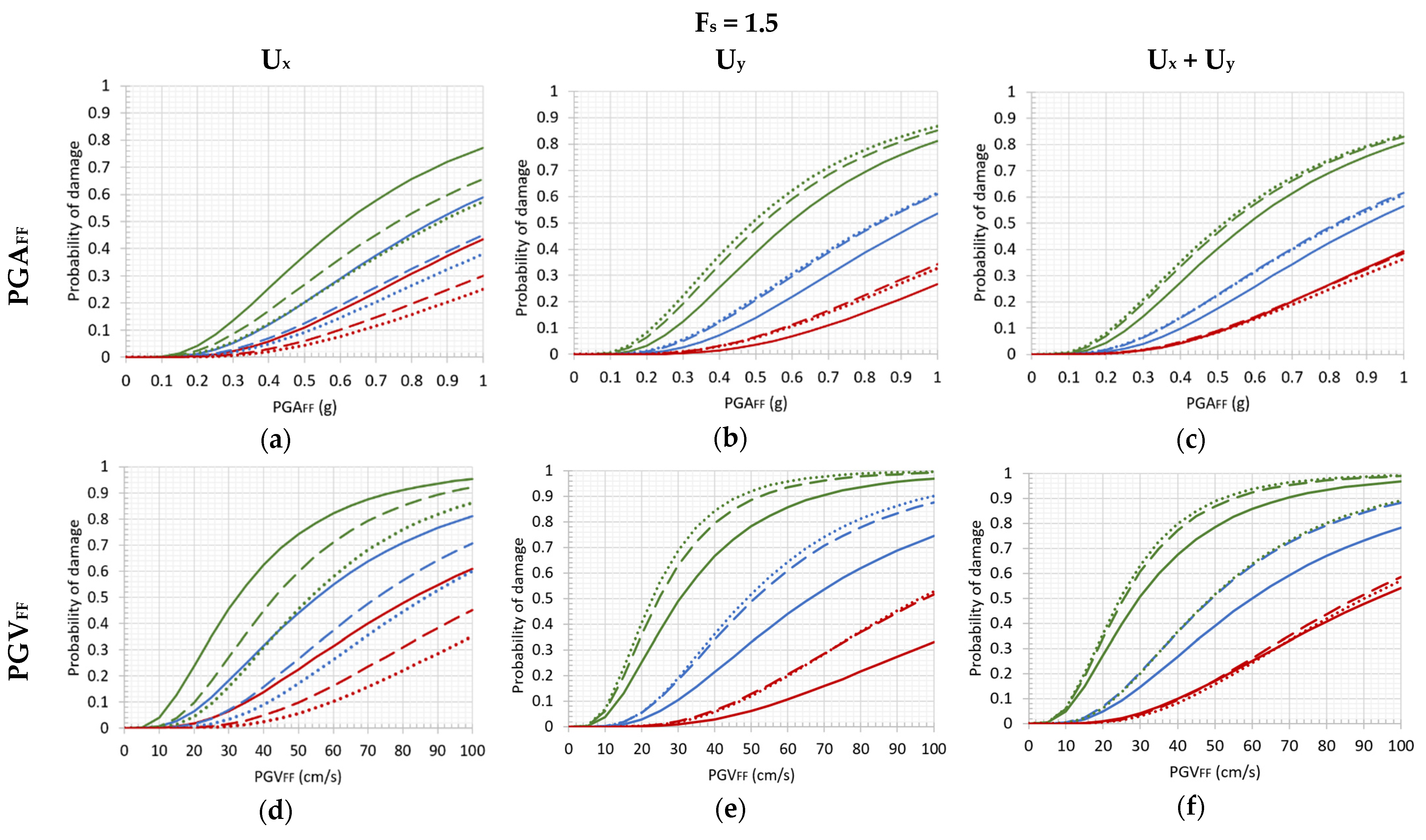
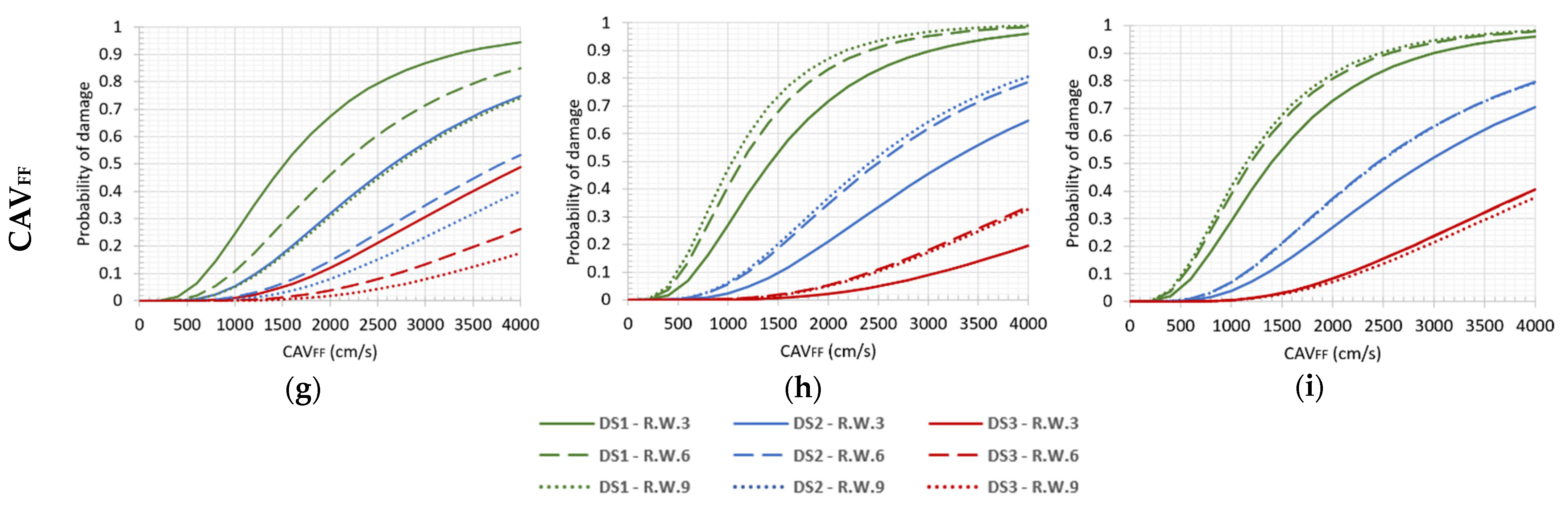

Figure A2.
Fragility curves for cantilever retaining walls R.W.3, R.W.6, R.W.9, regarding the case of initial condition Fs = 1.4, in terms of (a) PGAFF − Ux; (b) PGAFF − Uy; (c) PGAFF − Ux + Uy; (d) PGVFF − Ux; (e) PGVFF − Uy; (f) PGVFF − Ux + Uy; (g) CAVFF − Ux; (h) CAVFF − Uy; (i) CAVFF − Ux + Uy.
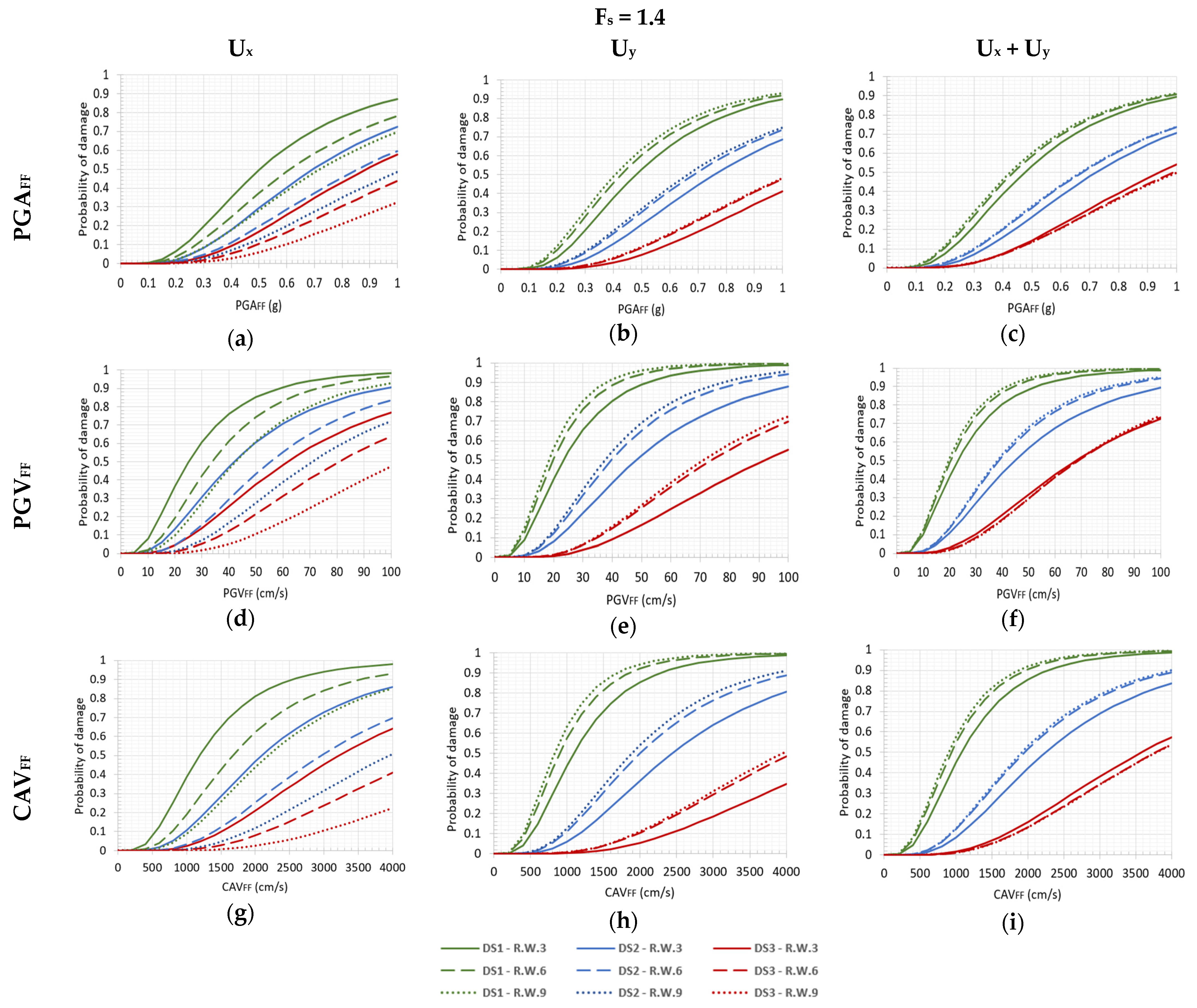
Figure A3.
Fragility curves for cantilever retaining walls R.W.3, R.W.6, R.W.9, regarding the case of initial condition Fs = 1.3, in terms of (a) PGAFF − Ux; (b) PGAFF − Uy; (c) PGAFF − Ux + Uy; (d) PGVFF − Ux; (e) PGVFF − Uy; (f) PGVFF − Ux + Uy; (g) CAVFF − Ux; (h) CAVFF − Uy; (i) CAVFF − Ux + Uy.
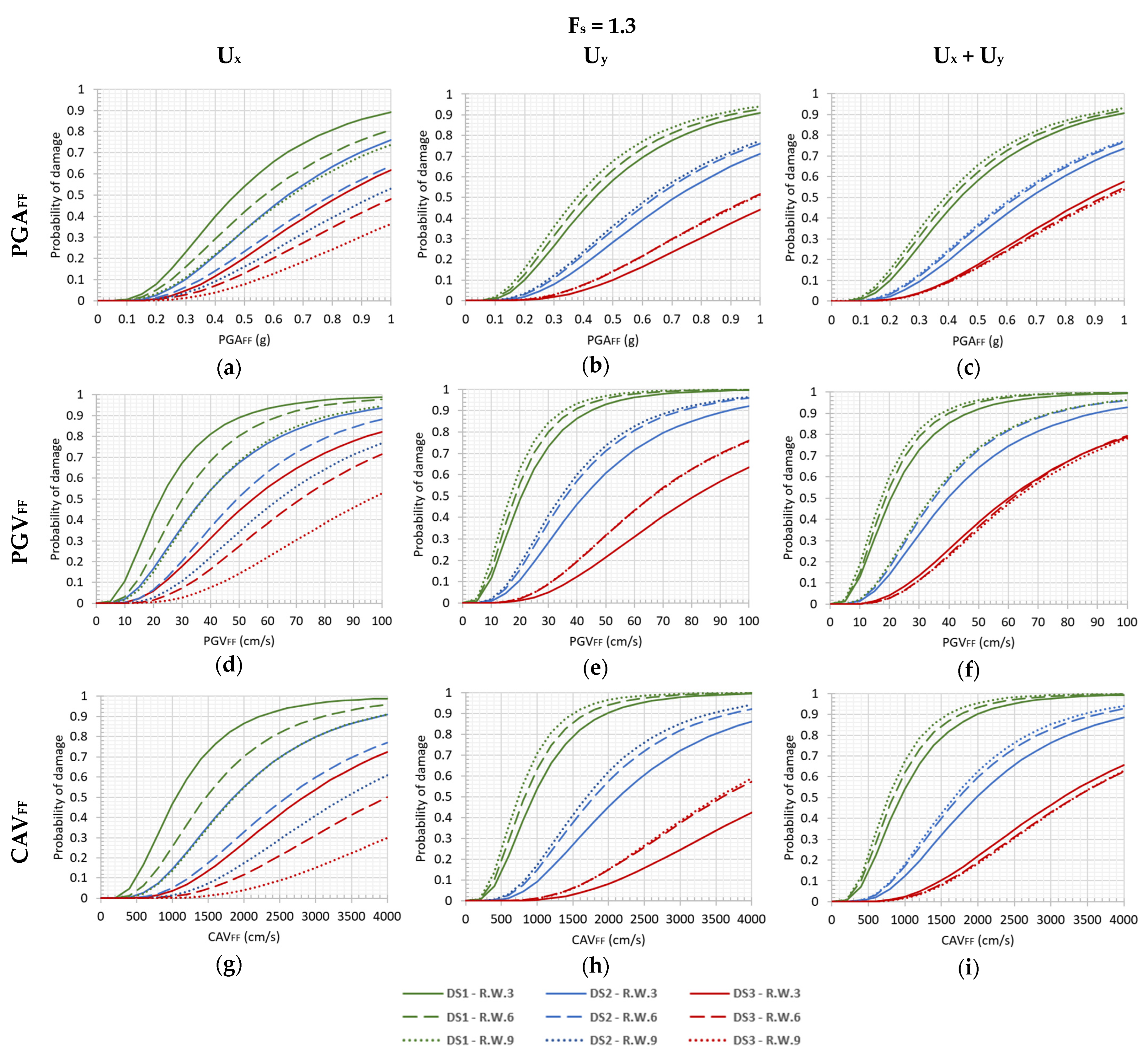
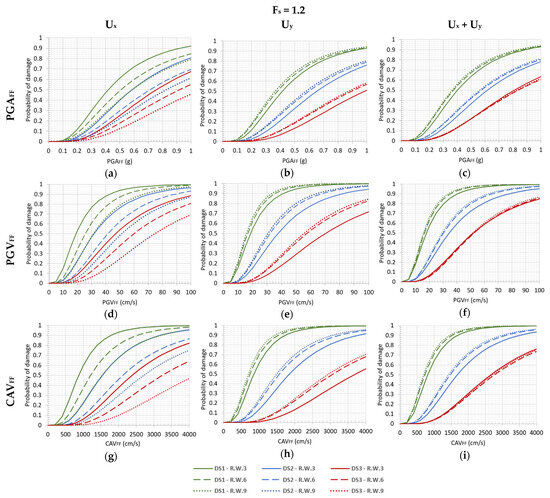
Figure A4.
Fragility curves for cantilever retaining walls R.W.3, R.W.6, R.W.9, regarding the case of initial condition Fs = 1.2, in terms of (a) PGAFF − Ux; (b) PGAFF − Uy; (c) PGAFF − Ux + Uy; (d) PGVFF − Ux; (e) PGVFF − Uy; (f) PGVFF − Ux + Uy; (g) CAVFF − Ux; (h) CAVFF − Uy; (i) CAVFF − Ux + Uy.
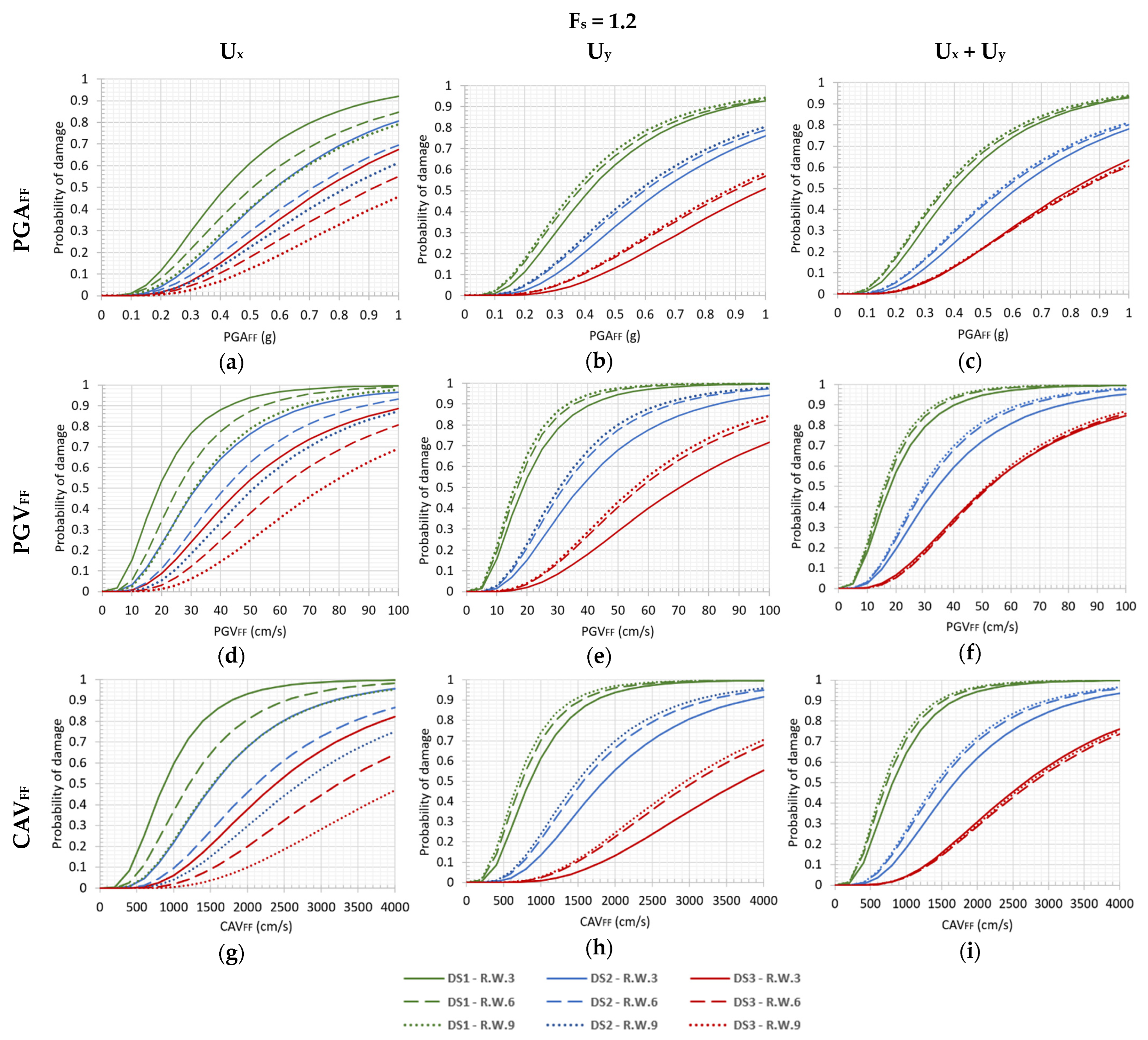
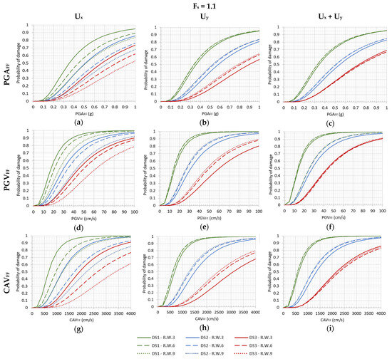
Figure A5.
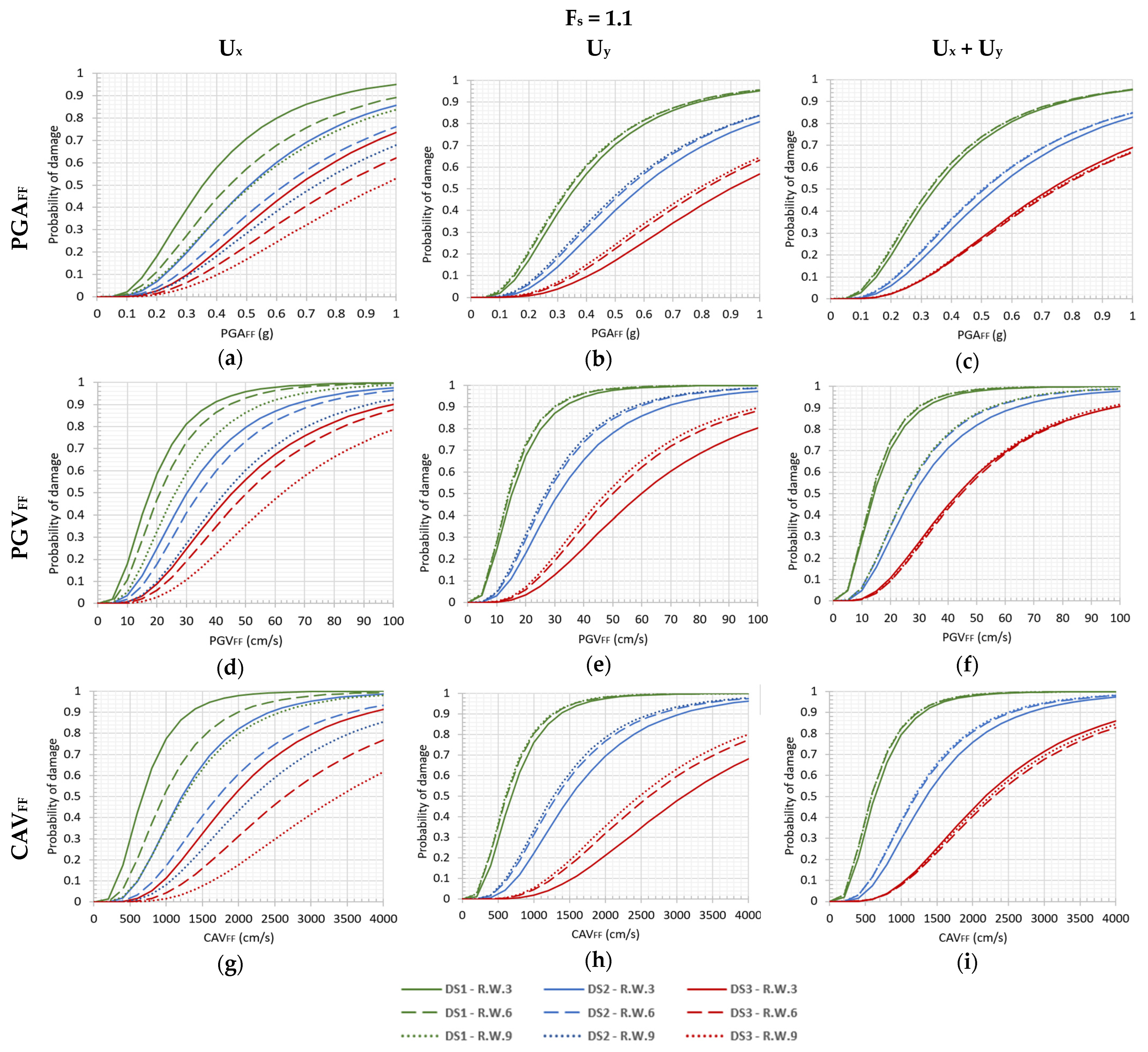
Fragility curves for cantilever retaining walls R.W.3, R.W.6, R.W.9, regarding the case of initial condition Fs = 1.1, in terms of (a) PGAFF − Ux; (b) PGAFF − Uy; (c) PGAFF − Ux + Uy; (d) PGVFF − Ux; (e) PGVFF − Uy; (f) PGVFF − Ux + Uy; (g) CAVFF − Ux; (h) CAVFF − Uy; (i) CAVFF − Ux + Uy.
Figure A5.
Fragility curves for cantilever retaining walls R.W.3, R.W.6, R.W.9, regarding the case of initial condition Fs = 1.1, in terms of (a) PGAFF − Ux; (b) PGAFF − Uy; (c) PGAFF − Ux + Uy; (d) PGVFF − Ux; (e) PGVFF − Uy; (f) PGVFF − Ux + Uy; (g) CAVFF − Ux; (h) CAVFF − Uy; (i) CAVFF − Ux + Uy.
Appendix C
For the comparative assessment of fragility curves referring to different initial conditions, Figure A6, Figure A7, Figure A8, Figure A9, Figure A10, Figure A11, Figure A12, Figure A13 and Figure A14 are provided, regarding the intensity measures PGAFF, PGVFF, and CAVFF, and the damage indices Ux, Uy, and Ux + Uy. Each figure corresponds to a different case of IM−DI, while each plot refers to an individual soil-wall model at a certain damage state.
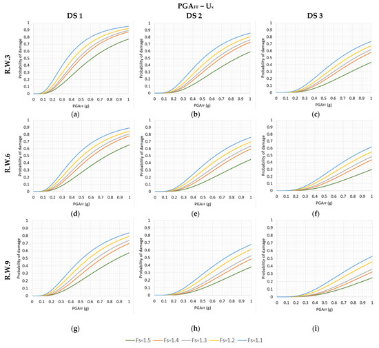
Figure A6.
Fragility curves for different initial conditions regarding the value of Fs = 1.1–1.5, in terms of PGA − Ux, for the cases of (a) R.W.3 − DS1; (b) R.W.3 − DS2; (c) R.W.3 − DS3; (d) R.W.6 − DS1; (e) R.W.6 − DS2; (f) R.W.6 − DS3; (g) R.W.9 − DS1; (h) R.W.9 − DS2; (i) R.W.9 − DS3.
Figure A6.
Fragility curves for different initial conditions regarding the value of Fs = 1.1–1.5, in terms of PGA − Ux, for the cases of (a) R.W.3 − DS1; (b) R.W.3 − DS2; (c) R.W.3 − DS3; (d) R.W.6 − DS1; (e) R.W.6 − DS2; (f) R.W.6 − DS3; (g) R.W.9 − DS1; (h) R.W.9 − DS2; (i) R.W.9 − DS3.
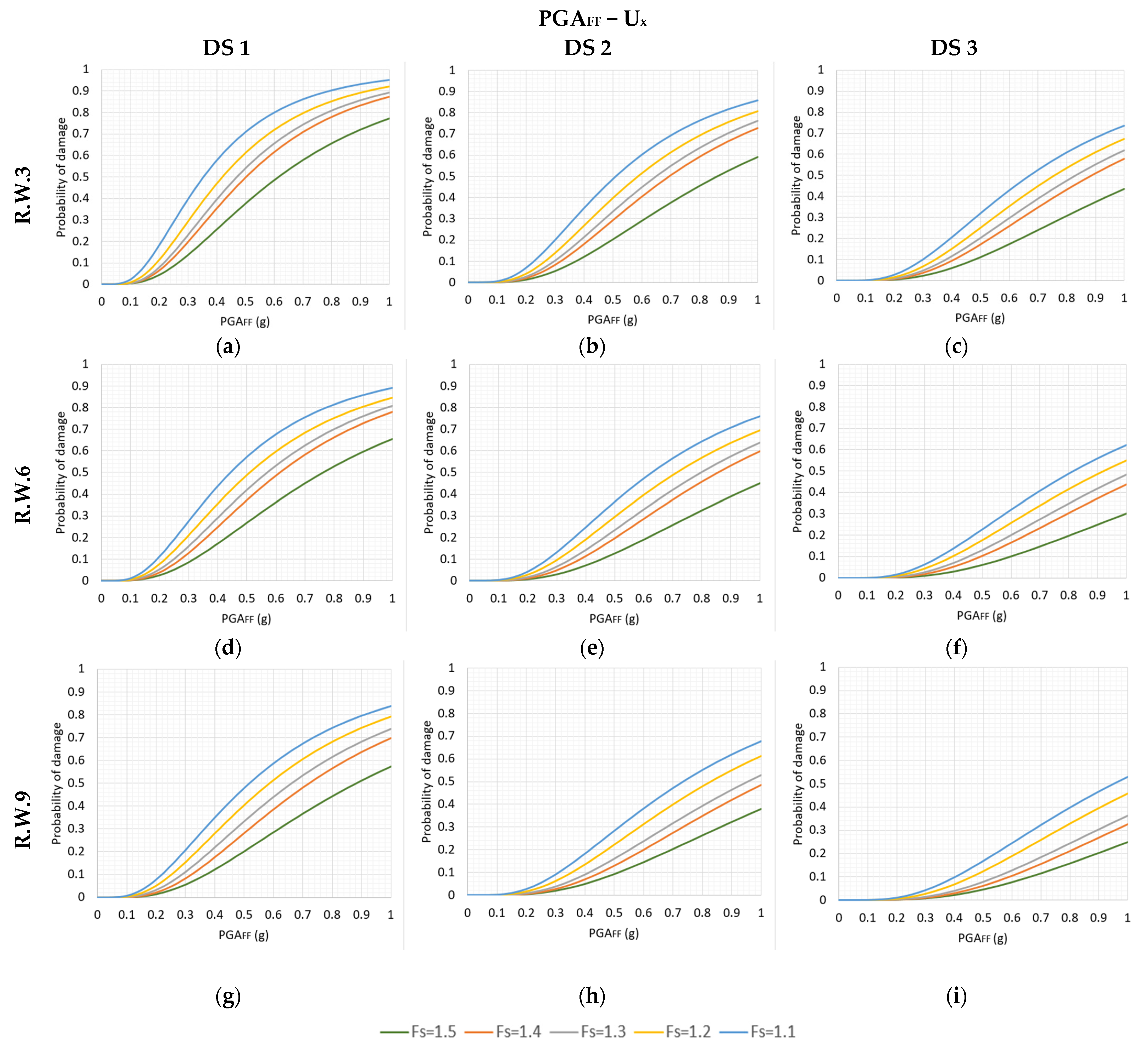
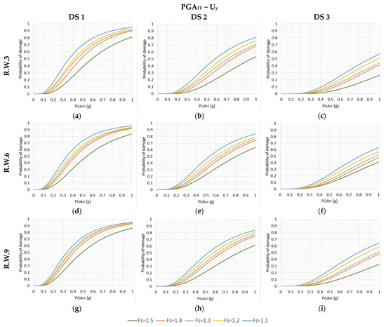
Figure A7.
Fragility curves for different initial conditions regarding the value of Fs = 1.1–1.5, in terms of PGA − Uy, for the cases of (a) R.W.3 − DS1; (b) R.W.3 − DS2; (c) R.W.3 − DS3; (d) R.W.6 − DS1; (e) R.W.6 − DS2; (f) R.W.6 − DS3; (g) R.W.9 − DS1; (h) R.W.9 − DS2; (i) R.W.9 − DS3.
Figure A7.
Fragility curves for different initial conditions regarding the value of Fs = 1.1–1.5, in terms of PGA − Uy, for the cases of (a) R.W.3 − DS1; (b) R.W.3 − DS2; (c) R.W.3 − DS3; (d) R.W.6 − DS1; (e) R.W.6 − DS2; (f) R.W.6 − DS3; (g) R.W.9 − DS1; (h) R.W.9 − DS2; (i) R.W.9 − DS3.
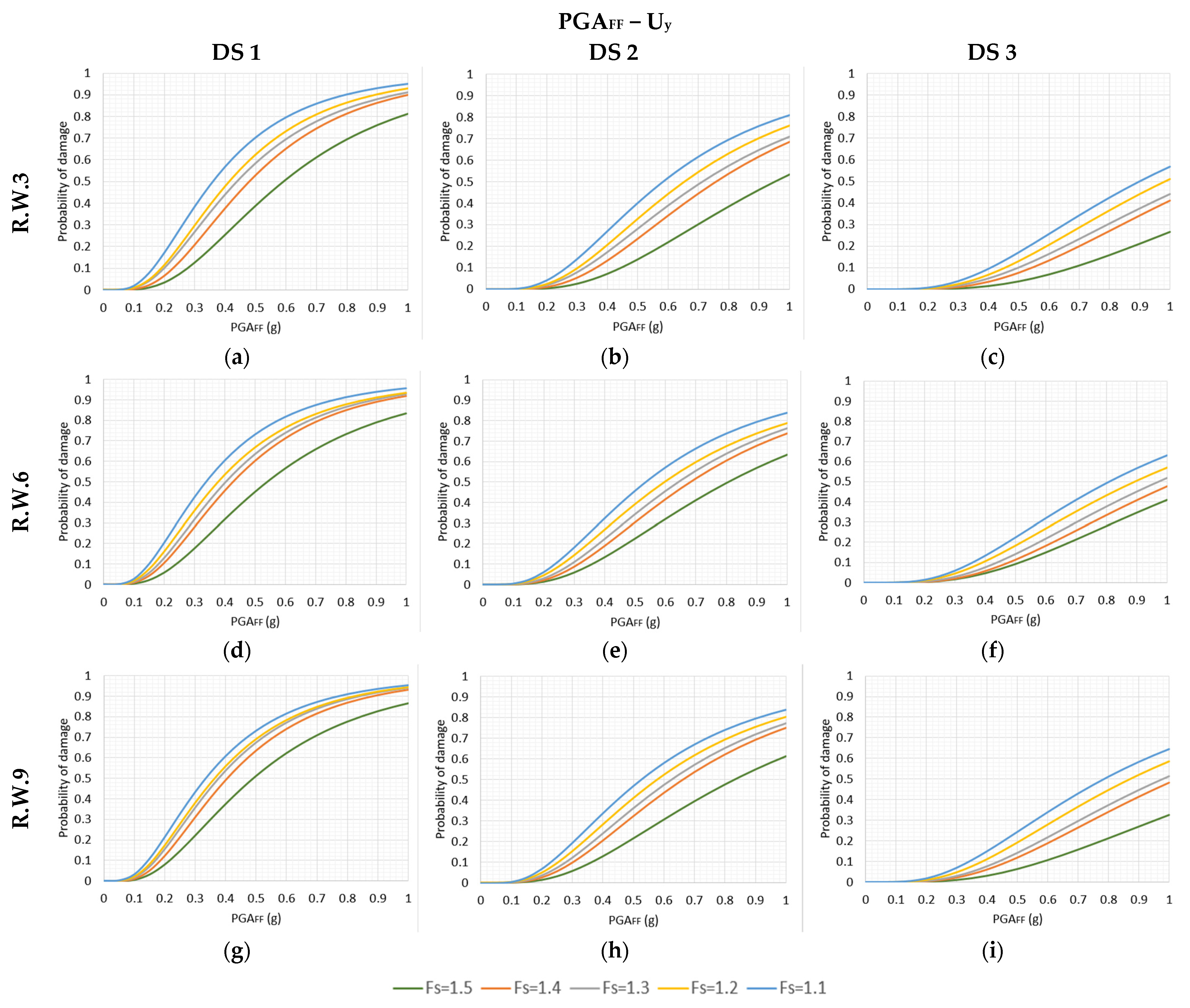
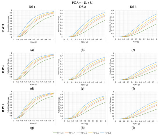
Figure A8.
Fragility curves for different initial conditions regarding the value of Fs = 1.1–1.5, in terms of PGA − Ux + Uy, for the cases of (a) R.W.3 − DS1; (b) R.W.3 − DS2; (c) R.W.3 − DS3; (d) R.W.6 − DS1; (e) R.W.6 − DS2; (f) R.W.6 − DS3; (g) R.W.9 − DS1; (h) R.W.9 − DS2; (i) R.W.9 − DS3.
Figure A8.
Fragility curves for different initial conditions regarding the value of Fs = 1.1–1.5, in terms of PGA − Ux + Uy, for the cases of (a) R.W.3 − DS1; (b) R.W.3 − DS2; (c) R.W.3 − DS3; (d) R.W.6 − DS1; (e) R.W.6 − DS2; (f) R.W.6 − DS3; (g) R.W.9 − DS1; (h) R.W.9 − DS2; (i) R.W.9 − DS3.
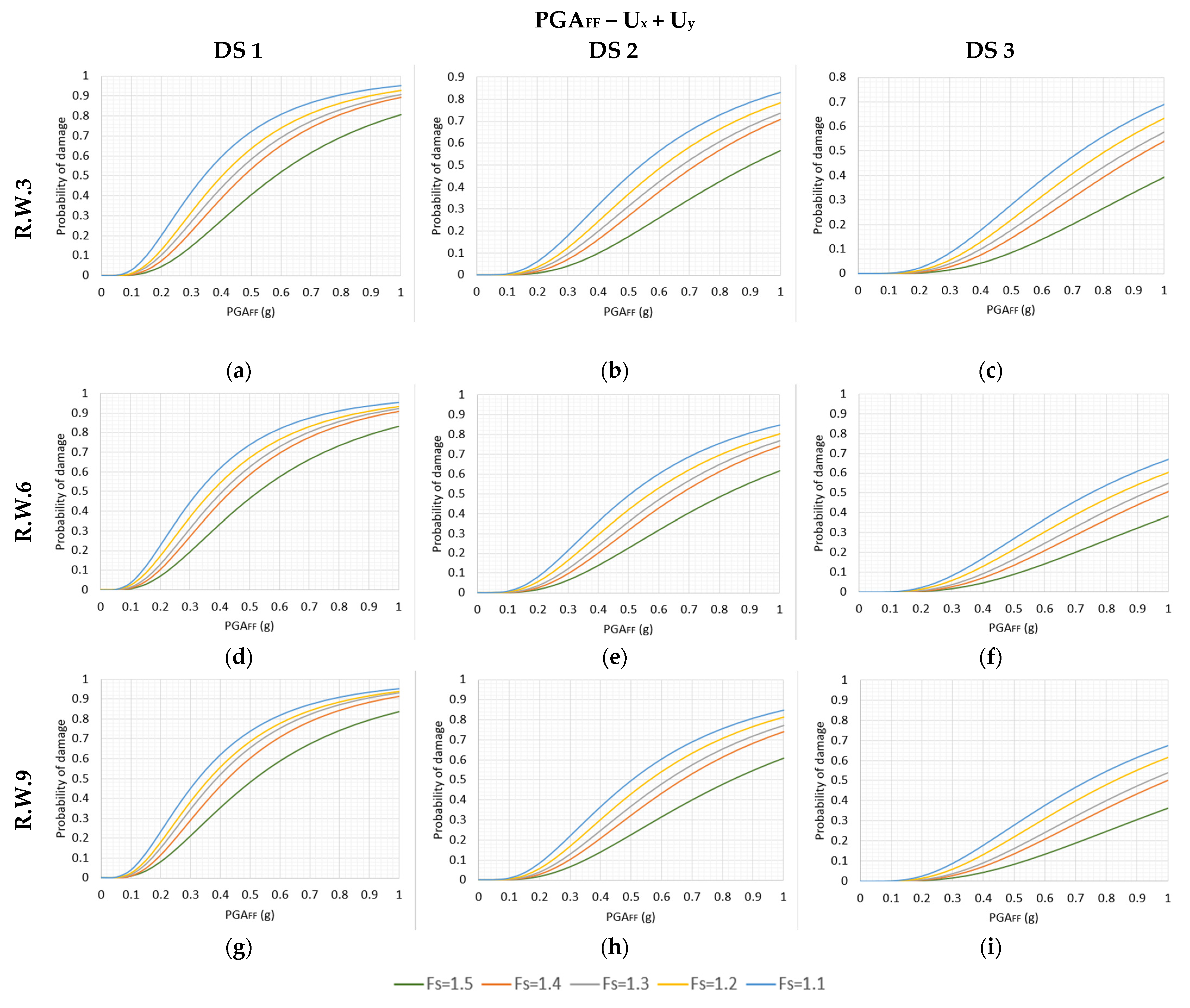
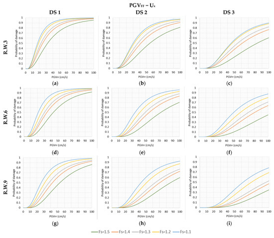
Figure A9.
Fragility curves for different initial conditions regarding the value of Fs = 1.1–1.5, in terms of PGV − Ux, for the cases of (a) R.W.3 − DS1; (b) R.W.3 − DS2; (c) R.W.3 − DS3; (d) R.W.6 − DS1; (e) R.W.6 − DS2; (f) R.W.6 − DS3; (g) R.W.9 − DS1; (h) R.W.9 − DS2; (i) R.W.9 − DS3.
Figure A9.
Fragility curves for different initial conditions regarding the value of Fs = 1.1–1.5, in terms of PGV − Ux, for the cases of (a) R.W.3 − DS1; (b) R.W.3 − DS2; (c) R.W.3 − DS3; (d) R.W.6 − DS1; (e) R.W.6 − DS2; (f) R.W.6 − DS3; (g) R.W.9 − DS1; (h) R.W.9 − DS2; (i) R.W.9 − DS3.
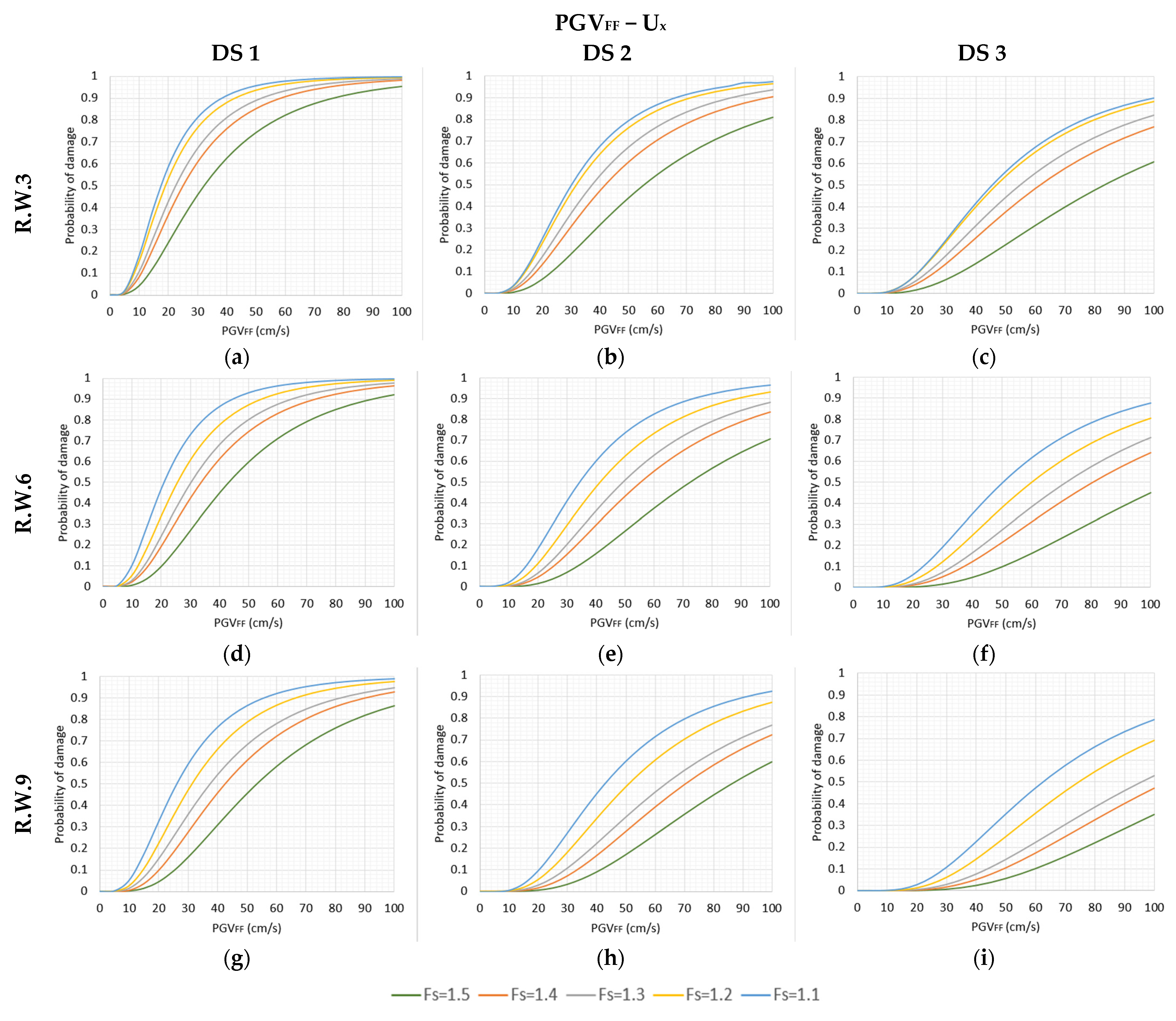
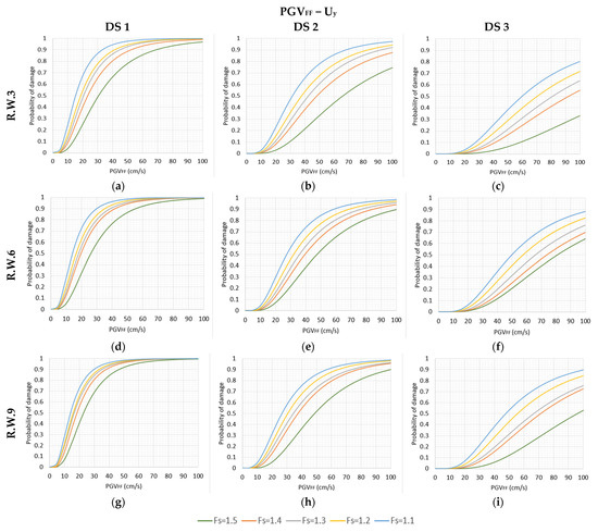
Figure A10.
Fragility curves for different initial conditions regarding the value of Fs = 1.1–1.5, in terms of PGV − Uy, for the cases of (a) R.W.3 − DS1; (b) R.W.3 − DS2; (c) R.W.3 − DS3; (d) R.W.6 − DS1; (e) R.W.6 − DS2; (f) R.W.6 − DS3; (g) R.W.9 − DS1; (h) R.W.9 − DS2; (i) R.W.9 − DS3.
Figure A10.
Fragility curves for different initial conditions regarding the value of Fs = 1.1–1.5, in terms of PGV − Uy, for the cases of (a) R.W.3 − DS1; (b) R.W.3 − DS2; (c) R.W.3 − DS3; (d) R.W.6 − DS1; (e) R.W.6 − DS2; (f) R.W.6 − DS3; (g) R.W.9 − DS1; (h) R.W.9 − DS2; (i) R.W.9 − DS3.
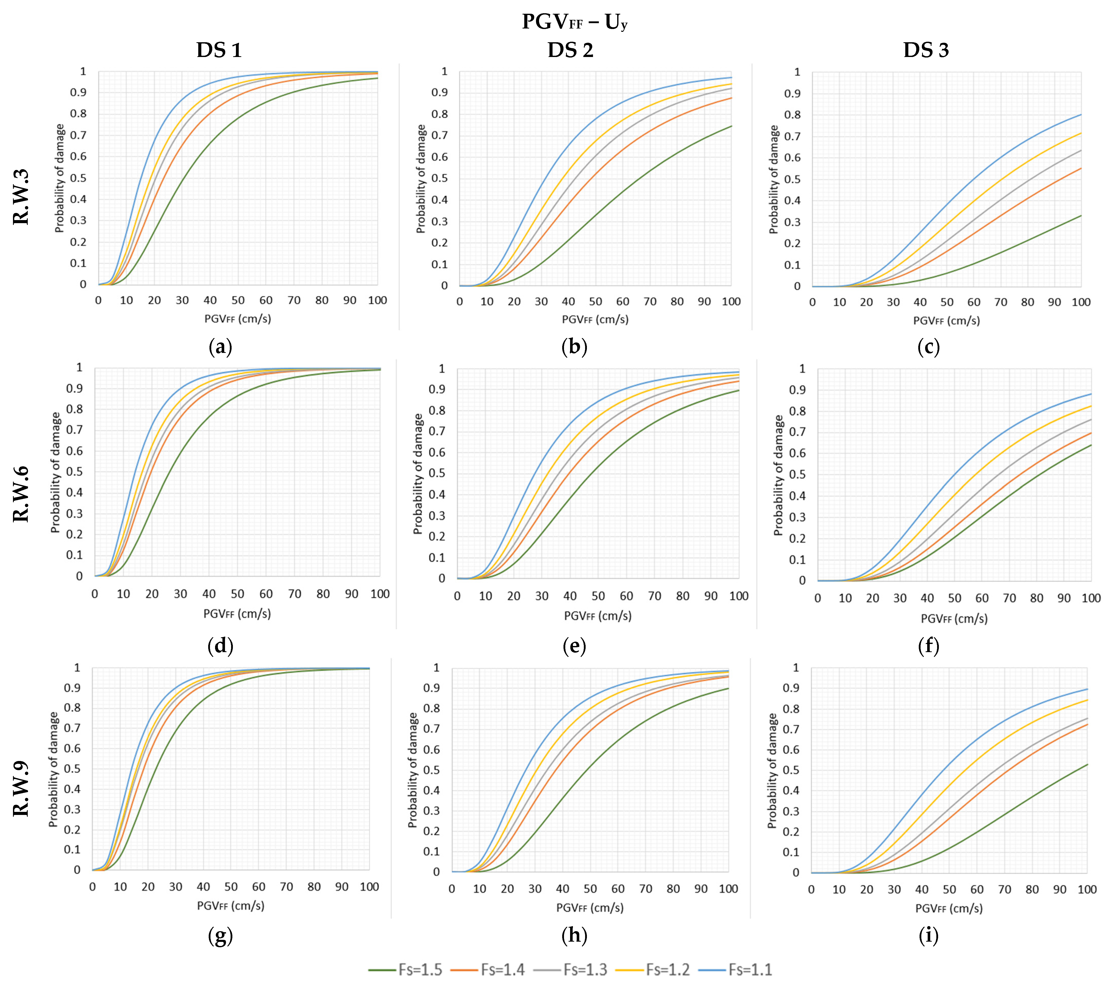
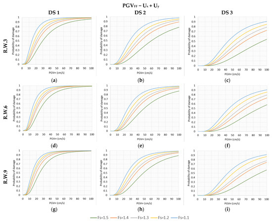
Figure A11.
Fragility curves for different initial conditions regarding the value of Fs = 1.1–1.5, in terms of PGV − Ux + Uy, for the cases of (a) R.W.3 − DS1; (b) R.W.3 − DS2; (c) R.W.3 − DS3; (d) R.W.6 − DS1; (e) R.W.6 − DS2; (f) R.W.6 − DS3; (g) R.W.9 − DS1; (h) R.W.9 − DS2; (i) R.W.9 − DS3.
Figure A11.
Fragility curves for different initial conditions regarding the value of Fs = 1.1–1.5, in terms of PGV − Ux + Uy, for the cases of (a) R.W.3 − DS1; (b) R.W.3 − DS2; (c) R.W.3 − DS3; (d) R.W.6 − DS1; (e) R.W.6 − DS2; (f) R.W.6 − DS3; (g) R.W.9 − DS1; (h) R.W.9 − DS2; (i) R.W.9 − DS3.
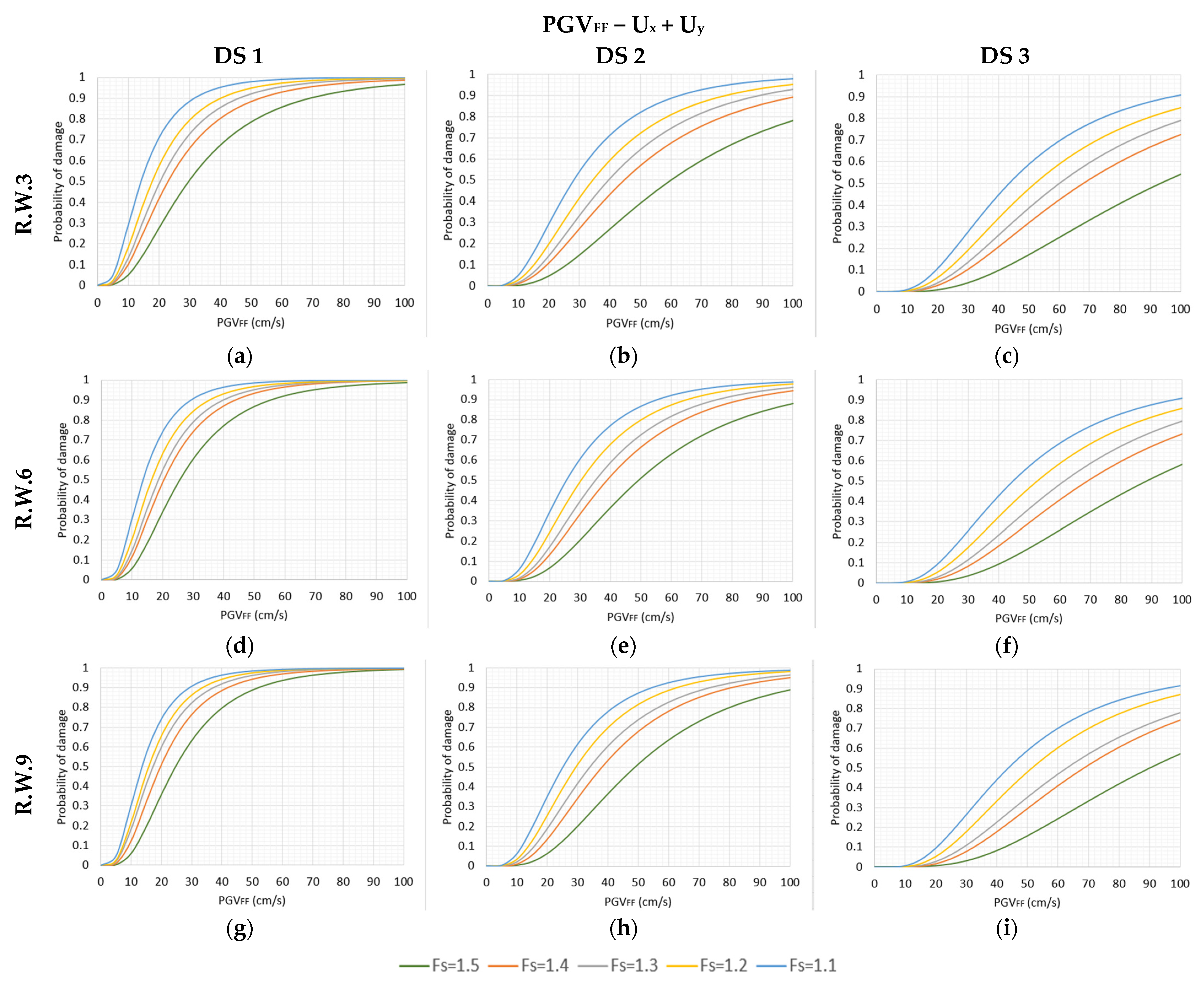
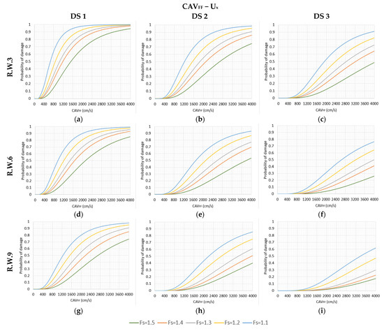
Figure A12.
Fragility curves for different initial conditions regarding the value of Fs = 1.1–1.5, in terms of CAV − Ux, for the cases of (a) R.W.3 − DS1; (b) R.W.3 − DS2; (c) R.W.3 − DS3; (d) R.W.6 − DS1; (e) R.W.6 − DS2; (f) R.W.6 − DS3; (g) R.W.9 − DS1; (h) R.W.9 − DS2; (i) R.W.9 − DS3.
Figure A12.
Fragility curves for different initial conditions regarding the value of Fs = 1.1–1.5, in terms of CAV − Ux, for the cases of (a) R.W.3 − DS1; (b) R.W.3 − DS2; (c) R.W.3 − DS3; (d) R.W.6 − DS1; (e) R.W.6 − DS2; (f) R.W.6 − DS3; (g) R.W.9 − DS1; (h) R.W.9 − DS2; (i) R.W.9 − DS3.
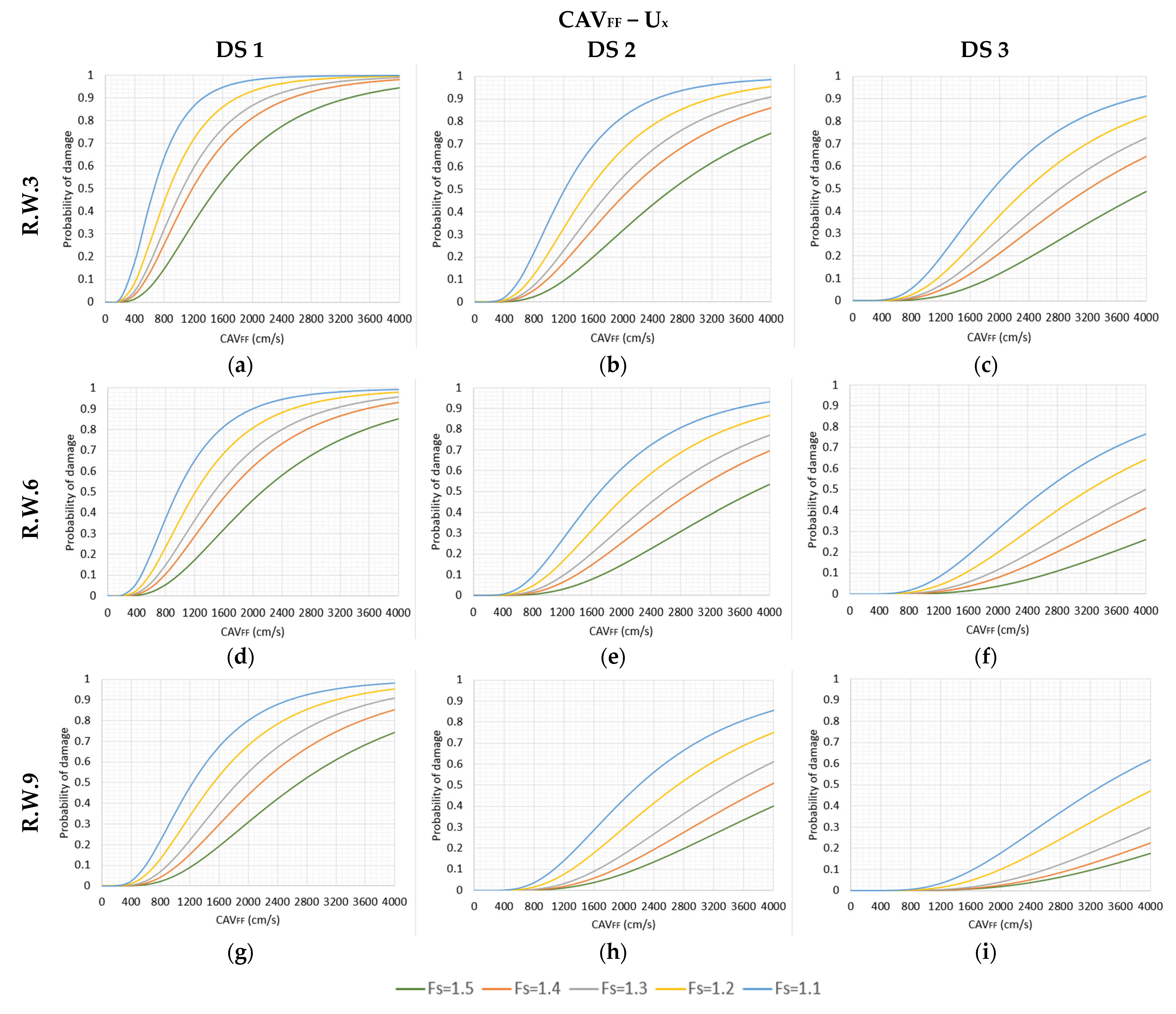
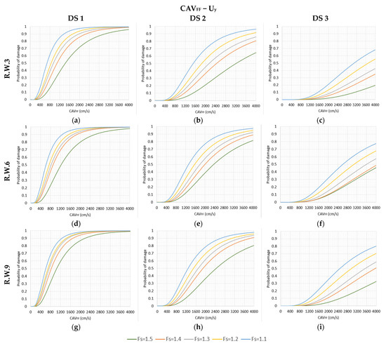
Figure A13.
Fragility curves for different initial conditions regarding the value of Fs = 1.1–1.5, in terms of CAV − Uy, for the cases of (a) R.W.3 − DS1; (b) R.W.3 − DS2; (c) R.W.3 − DS3; (d) R.W.6 − DS1; (e) R.W.6 − DS2; (f) R.W.6 − DS3; (g) R.W.9 − DS1; (h) R.W.9 − DS2; (i) R.W.9 − DS3.
Figure A13.
Fragility curves for different initial conditions regarding the value of Fs = 1.1–1.5, in terms of CAV − Uy, for the cases of (a) R.W.3 − DS1; (b) R.W.3 − DS2; (c) R.W.3 − DS3; (d) R.W.6 − DS1; (e) R.W.6 − DS2; (f) R.W.6 − DS3; (g) R.W.9 − DS1; (h) R.W.9 − DS2; (i) R.W.9 − DS3.
Figure A14.
Fragility curves for different initial conditions regarding the value of Fs = 1.1–1.5, in terms of CAV − Ux + Uy, for the cases of (a) R.W.3 − DS1; (b) R.W.3 − DS2; (c) R.W.3 − DS3; (d) R.W.6 − DS1; (e) R.W.6 − DS2; (f) R.W.6 − DS3; (g) R.W.9 − DS1; (h) R.W.9 − DS2; (i) R.W.9 − DS3.
Figure A14.
Fragility curves for different initial conditions regarding the value of Fs = 1.1–1.5, in terms of CAV − Ux + Uy, for the cases of (a) R.W.3 − DS1; (b) R.W.3 − DS2; (c) R.W.3 − DS3; (d) R.W.6 − DS1; (e) R.W.6 − DS2; (f) R.W.6 − DS3; (g) R.W.9 − DS1; (h) R.W.9 − DS2; (i) R.W.9 − DS3.
References
- Akai, K.; Bray, J.; Boulanger, R.; Christian, J.; Finn, L.; Harder, L.; Idriss, I.; Ishihara, K.; Iwasaki, Y.; Mitchell, J.; et al. Geotechnical Reconnaissance of the Effects of the January 17, 1995 Hyogoken-Nanbu Earthquake, Japan; Report No. UCB/EERC-95/01; Earthquake Engineering Research Center, College of Engineering, University of California: Berkeley, CA, USA, 1995. [Google Scholar]
- Abrahamson, N.; Bardet, J.P.; Boulanger, R.; Bray, J.; Chan, Y.-W.; Chang, C.-Y.; Chen, C.-H.; Harder, L.; Huang, A.-B.; Huang, S.; et al. Preliminary Geotechnical Earthquake Engineering Observations of the September 21, 1999, Ji-Ji, Taiwan Earthquake; Geotechnical Extreme Events Reconnaissance (GEER) Association Report 002; 8 October 1999; Available online: https://geerassociation.org/ (accessed on 19 October 2023).
- Rollins, K.; Ledezma, C.; Montalva, G. Geotechnical Aspects of April 1, 2014, M8.2 Iquique, Chile Earthquake; Geotechnical Extreme Events Reconnaissance (GEER) Association Report 038; Version 1.2: 22 October 2014. Available online: https://geerassociation.org/components/com_geer_reports/geerfiles/Iquique_Chile_GEER_Report.pdf (accessed on 19 October 2023).
- Nikolaou, S.; Zekkos, D.; Assimaki, D.; Gilsanz, R. Earthquake Reconnaissance January 26th/February 2nd 2014, Cephalonia, Greece Events; Geotechnical Extreme Events Reconnaissance (GEER) Report 034; GEER/EERI/ATC; 2014; Available online: https://www.geoengineer.org/news/geer-reconnaissance-report-cephalonia-island-greece-earthquakes-2014 (accessed on 19 October 2023).
- Stewart, J.; Lanzo, G.; Aversa, S.; Bozzoni, F.; Chiabrando, F.; Grasso, N.; Dashti, S.; Di Sarno, L.; Durante, M.G.; Foti, S.; et al. Engineering Reconnaissance Following the 2016 M 6.0 Central Italy Earthquake; Geotechnical Extreme Events Reconnaissance (GEER) Association Report 050; 2016; Available online: https://geerassociation.org/components/com_geer_reports/geerfiles/Central_Italy_GEER_Report_Ver1.pdf (accessed on 19 October 2023).
- Çen, Ö.; Bray, J.; Frost, D.; Hortacsu, A.; Miranda, E.; Moss, R.E.; Stewart, J. February 6, 2023 Turkiye Earthquakes: Report on Geoscience and Engineering Impacts; Geotechnical Extreme Events Reconnaissance (GEER) Association Report 082; Earthquake Engineering Research Institute: Oakland, CA, USA, 2023. [Google Scholar] [CrossRef]
- Argyroudis, S.; Selva, J.; Gehl, P.; Pitilakis, K. Systemic Seismic Risk Assessment of Road Networks Considering Interactions with the Built Environment. Comput. Aided Civ. Infrastruct. Eng. 2015, 30, 524–540. [Google Scholar] [CrossRef]
- National Institute of Building Sciences. HAZUS-MH: Users’ and Technical Manuals; Federal Emergency Management Agency: Washington, DC, USA, 2004.
- Erberik, M.A. Seismic Fragility Analysis. In Encyclopedia of Earthquake Engineering; Beer, M., Kougioumtzoglou, I., Patelli, E., Au, I.K., Eds.; Springer: Berlin/Heidelberg, Germany, 2015; pp. 1–10. [Google Scholar]
- Prakash, S.; Wu, Y.; Rafnsson, E.A. On seismic design displacements of rigid retaining walls. In Proceedings of the Third International Conference on Recent Advances in Geotechnical Earthquake Engineering and Soil Dynamics, St. Louis, MO, USA, 2–7 April 1995. [Google Scholar]
- Huang, C.-C.; Wu, S.H.; Wu, H.J. Seismic displacement criterion for soil retaining walls based on soil strength mobilization. J. Geotech. Geoenviron. Eng. 2009, 135, 74–83. [Google Scholar] [CrossRef]
- Zamiran, S.; Osouli, A. Seismic motion response and fragility analyses of cantilever retaining walls with cohesive backfill. Soils Found. 2018, 58, 412–426. [Google Scholar] [CrossRef]
- Cosentini, R.M.; Bozzoni, F. Fragility curves for rapid assessment of earthquake-induced damage to earth-retaining walls starting from optimal seismic intensity measures. Soil Dyn. Earthq. Eng. 2022, 152, 107017. [Google Scholar] [CrossRef]
- Seo, H.; Lee, Y.-J.; Park, D.; Kim, B. Seismic fragility assessment for cantilever retaining walls with various backfill slopes in South Korea. Soil Dyn. Earthq. Eng. 2022, 161, 107443. [Google Scholar] [CrossRef]
- Argyroudis, S.; Kaynia, A.M.; Pitilakis, K. Development of fragility functions for geotechnical constructions: Application to cantilever retaining walls. Soil Dyn. Earthq. Eng. 2013, 50, 106–116. [Google Scholar] [CrossRef]
- Kaynia, M.A.; Argyroudis, S.; Mayoral, J.M.; Johansson, J.; Pitilakis, K.; Anastasiadis, A. D3.7: Fragility functions for roadway system elements. In SYNER-G: Systemic Seismic Vulnerability and Risk Analysis for Buildings, Lifeline Networks and Infrastructures Safety Gain, FP7-ENV-2009-1-244061; 2011; Available online: https://www.vce.at/SYNER-G/pdf/deliverables/D3.07_Fragility%20functions%20for%20roadway%20system%20elements.pdf (accessed on 19 October 2023).
- PIANC. Seismic Design Guidelines for Port Structures. In Working Group 34 of the Maritime Navigation Commission; International Navigation Association; Balkema: Rotterdam, The Netherlands, 2001. [Google Scholar]
- EN 1998–1; EC8 Eurocode 8: Design of Structures for Earthquake Resistance. European Committee for Standardisation: Brussels, Belgium, 2004.
- PLAXIS 2D. Reference Manual, Version 1; Bentley Systems: Delft, The Netherlands, 2023. [Google Scholar]
- Itasca, I. FLAC-Fast Lagrangian Analysis of Continua, Version 7.0; Itasca Consulting Group: Minneapolis, MN, USA, 2011. [Google Scholar]
- Han, S.; Wei, X.; Yang, K.; Yun, L.; Cheng, C. Influence of Water Level Change on Deformation and Stability of Retaining Walls with Different Back Materials. Adv. Eng. Res. 2016, 63, 296–300. [Google Scholar] [CrossRef]
- Hardin, B.O.; Drnevich, V.P. Shear modulus and damping in soils: Design equations and curves. J. Soil Mech. Found. Div. 1972, 98, 667–692. [Google Scholar] [CrossRef]
- Brinkgreve, R.; Kappert, M.; Bonnier, P. Hysteretic damping in a small-strain stiffness model. In Proceedings of the Numerical Models in Geomechanics-NUMOG X, Rhodes, Greece, 25–27 April 2007. [Google Scholar] [CrossRef]
- Benz, T. Small-Strain Stiffness of Soils and Its Numerical Consequences. Ph.D. Thesis, University of Stuttgart, Stuttgart, Germany, 2007. [Google Scholar]
- Margaris, B.; Scordilis, E.; Stewart, J.; Boore, D.; Theodoulidis, N.; Kalogeras, I.; Melis, N.; Skarlatoudis, A.; Klimis, N.; Seyhan, E. Hellenic Strong-Motion Database with Uniformly Assigned Source and Site Metadata for the Period 1972–2015. Seismol. Res. Lett. 2021, 92, 2065–2080. [Google Scholar] [CrossRef]
- Sotiriadis, D.; Margaris, B.; Klimis, N.; Dokas, I. Seismic Hazard in Greece: A Comparative Study for the Region of East Macedonia and Thrace. GeoHazards 2023, 4, 239–266. [Google Scholar] [CrossRef]
- Che, F.; Yin, C.; Zhang, H.; Tang, G.; Hu, Z.; Liu, D.; Li, Y.; Huang, Z. Assesing the Risk Probability of the Embankment Seismic Damage Using Monte Carlo Method. Adv. Civ. Eng. 2020, 2020, 8839400. [Google Scholar] [CrossRef]
- Lesgidis, N.; Sextos, A.; Kwon, O.-S. Influence of frequency-dependent soil-structure interaction on the fragility of R/C bridges. Earthq. Eng. Struct. Dyn. 2016, 46, 139–158. [Google Scholar] [CrossRef]
- Kottke, A.R.; Rathje, E.M. Strata 2013. Available online: github.com/arkottke/strata (accessed on 15 June 2023).
- Darendeli, M.-B. Development of New Family of Normalized Modulus Reduction and Material Damping Curves. Ph.D. Thesis, University of Texas, Austin, TX, USA, 2001. [Google Scholar]
- Karakas, C.-C.; Palanci, M.; Senel, S.-M. Fragility based evaluation of different code based assessment approaches for the performance estimation of existing buildings. Bull. Earthq. Eng. 2022, 20, 1685–1716. [Google Scholar] [CrossRef]


Disclaimer/Publisher’s Note: The statements, opinions and data contained in all publications are solely those of the individual author(s) and contributor(s) and not of MDPI and/or the editor(s). MDPI and/or the editor(s) disclaim responsibility for any injury to people or property resulting from any ideas, methods, instructions or products referred to in the content. |
© 2023 by the authors. Licensee MDPI, Basel, Switzerland. This article is an open access article distributed under the terms and conditions of the Creative Commons Attribution (CC BY) license (https://creativecommons.org/licenses/by/4.0/).