Accurate Feature Extraction from Historical Geologic Maps Using Open-Set Segmentation and Detection

Abstract

This study presents a novel AI method for extracting polygon and point features from historical geologic maps, representing a pivotal step for assessing the mineral resources needed for energy transition. Our innovative method involves using map units in the legends as prompts for one-shot segmentation and detection in geological feature extraction. The model, integrated with a human-in-the-loop system, enables geologists to refine results efficiently, combining the power of AI with expert oversight. Tested on geologic maps annotated by USGS and DARPA for the AI4CMA DARPA Challenge, our approach achieved a median F1 score of 0.91 for polygon feature segmentation and 0.73 for point feature detection when such features had abundant annotated data, outperforming current benchmarks. By efficiently and accurately digitizing historical geologic map, our method promises to provide crucial insights for responsible policymaking and effective resource management in the global energy transition.

1. Introduction

Geologic maps are essential tools that visually represent the distribution of different rock types and unconsolidated minerals at or near the Earth’s surface by using distinct colors and patterns to convey information about the composition, age, and structure of these geologic units [1]. These maps detail the distribution of rock types, structures, and surface features that are critical for identifying regions favorable for mineral deposits. Despite their importance, the inclusion of geologic map data in mineral assessment is often hindered by the challenge of quickly digitizing historical geologic maps. Although there are approximately 100,000 scanned geologic maps in the USGS National Geologic Map Database (NGMDB) [2], only a few have been digitized in a manner suitable for proper mineral assessment. The manual digitization of these maps is a labor-intensive process, often taking days to weeks for a single map, and it poses a significant bottleneck in advancing the objectives of Earth MRI (Mineral Resources Initiative) [3]. To overcome this challenge, the use of image processing and AI technologies is essential, enabling the faster and more efficient digitization of geologic maps and thereby accelerating progress toward comprehensive critical mineral assessments.

Digitizing geologic maps has become increasingly urgent due to the vulnerable domestic supply chain of critical minerals. The transition to sustainable energy is critically dependent on the availability of critical minerals, such as lithium, copper, and uranium. The scarcity or absence of these critical minerals could severely hinder the development of sustainable energy solutions and threaten national economic stability. To mitigate the risks associated with potential supply chain disruptions, a comprehensive understanding of domestic mineral resources is imperative. This is where critical minerals assessment (CMA) becomes vital, as it helps identify vulnerabilities and secure the necessary materials for the future. The U.S. Geological Survey (USGS) has taken the lead in enhancing our understanding of the geologic framework across the United States through initiatives like the Earth MRI [3]. This program specifically aims to identify areas that may contain undiscovered critical mineral resources. By bolstering the domestic mineral supply, Earth MRI seeks to reduce the nation’s reliance on foreign sources of these essential minerals, which are fundamental to national security and economic well-being.

Initial efforts under Earth MRI have primarily concentrated on geophysical and geochemical data. Geophysical data provide insights into the subsurface by measuring physical properties such as magnetism, gravity, and electrical conductivity, enabling the detection of buried mineral deposits and a better understanding of the geological structures that control their formation. Geochemical data, including the analysis of bedrock and stream sediment, offer crucial information on the chemical composition of surface materials, aiding in the identification of elemental anomalies associated with critical minerals. The integration of geophysical and geochemical data with geologic maps enables the creation of comprehensive models of potential critical mineral deposits, and such multi-source data have been explored for mineral prospectivity mapping [4].

Digitizing geologic maps involves segmenting complex regions with overlapping layers, intertwined lines, and irregular geometries. This process requires manually tracing key points, lines, and polygons to create vector features and linking them to corresponding legend descriptions. Polygon features are essential, as they represent the physical, chemical, and geological components of mineral resources. These features are defined by the concentration of natural materials in quantities that determine the economic feasibility of extraction. Point symbols on geologic maps are also essential, and they can represent a variety of features, including the location of fossils, mineral occurrences, or sample sites. Unlike standard segmentation/detection tasks, this is challenging due to the frequent overlap, discontinuity, and varying shapes and sizes of features like polygons, points, lines, and text in mineral field maps. Additionally, the same feature type can be represented by different symbols or patterns across different maps, which is a problem known as “inconsistent symbology” [5]. This inconsistency, driven by changes in cartographic design over time, complicates the development of a universal identifier for features such as mine locations or mineral resource tracts. To facilitate polygon segmentation and point detection based on map units in the legend, we refer to the task as “prompt-based segmentation/detection”, where each map unit acts as a “prompt” to guide the model’s segmentation and detection processes. In this study, we developed a deep learning method to extract polygon/point features from scanned maps with inconsistent symbology. We developed a prompt-based model to help automate the feature extraction process. For our study, the map image and prompt image were concatenated into a 6-channel array to serve as the model input.

In summary, the inclusion of digitized geologic map data is vital for enhancing the accuracy and reliability of probabilistic estimates of undiscovered mineral resources. This initiative builds upon the most comprehensive mineral site compilation to date, serving as a crucial foundation for the development of the first national-scale mineral prospectivity maps. Moreover, this advanced toolset for identifying polygon and point features could also be valuable in other applications, such as the digitization of historical CAD drawings or chemical process diagrams.

The main contributions of this paper can be summarized as follows:

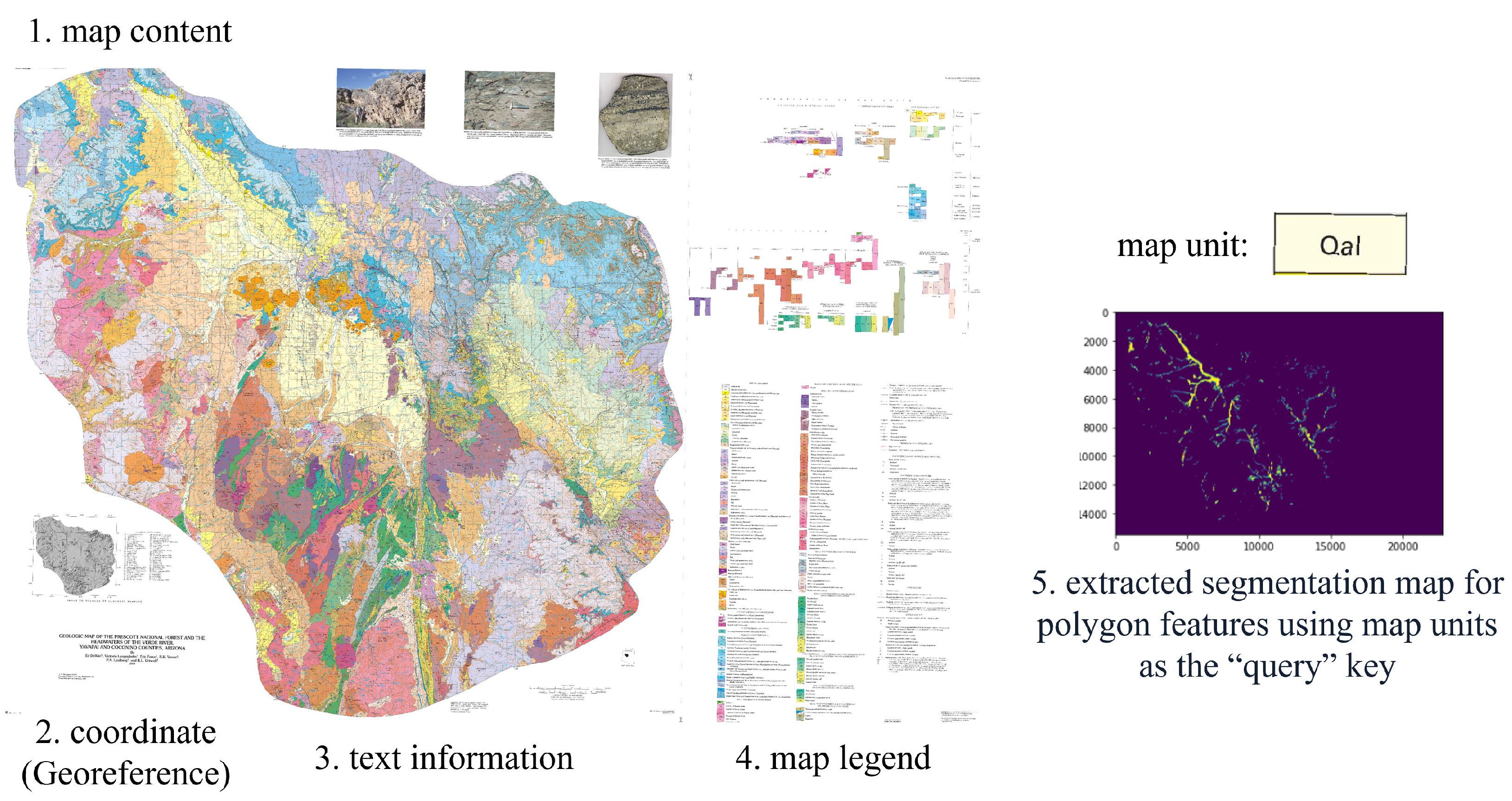
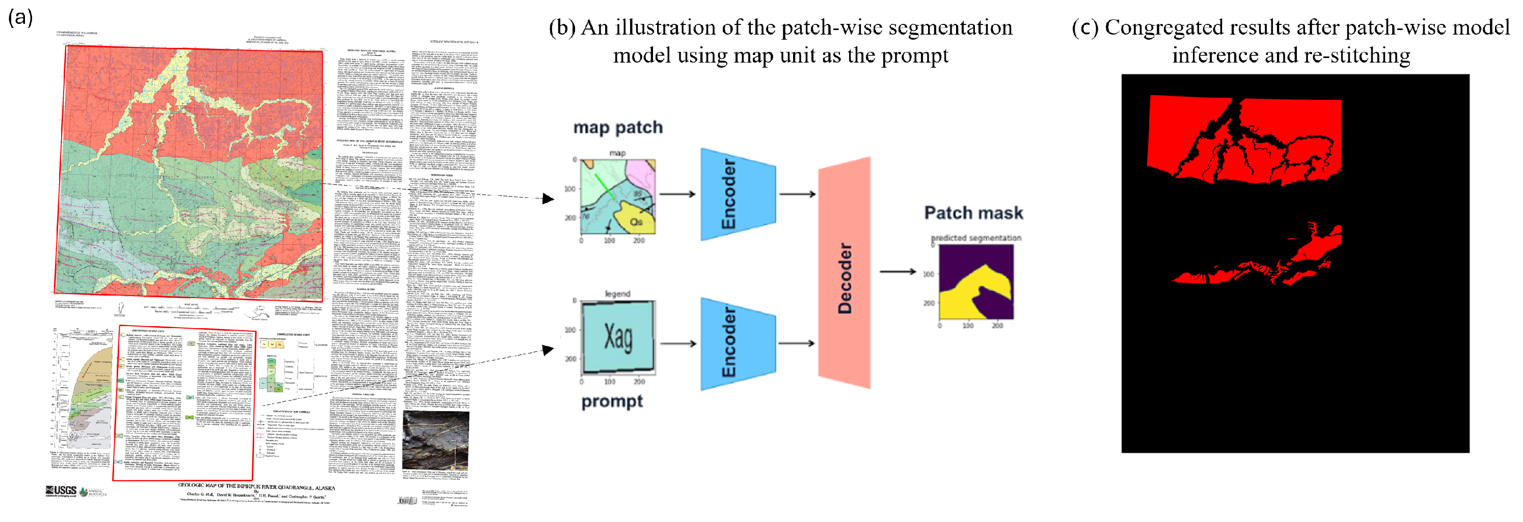
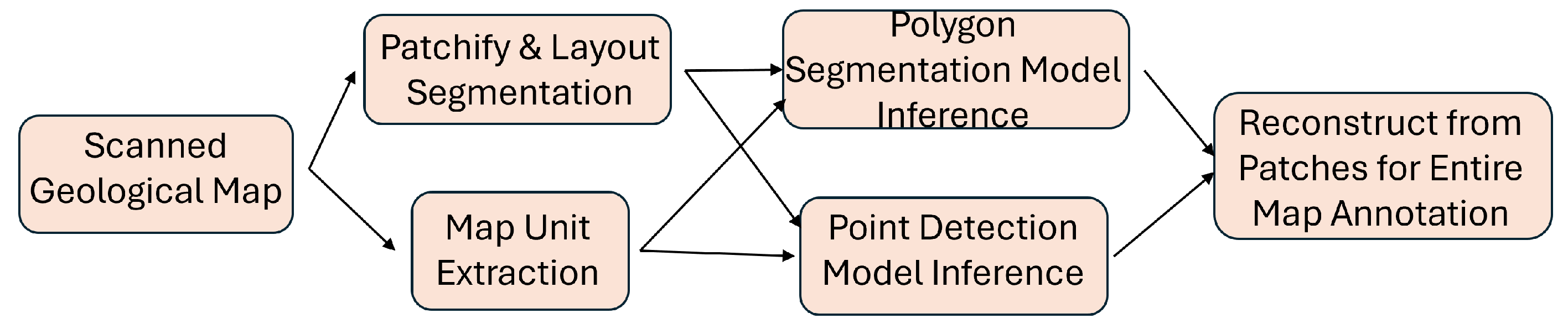
• We developed an automated pipeline for geologic map feature extraction. Initially, we extracted map units from the legend region, and then we used a prompt-based method for open-set polygon and point feature extraction, utilizing the legend items as prompts.
• We systematically evaluated the effects of patch size, model backbone, and data augmentation methods on model performance, including hyperparameter tuning, to enhance both accuracy and generalizability.
• We vectorized the extracted polygon and point features to facilitate their integration with geophysical and geochemical data, enabling multi-source mineral prospectivity mapping.

2. Related Work

2.1. Geologic Map Digitization

A geologic map is characterized by its detailed and large-scale representation of geographical features, including polygons, contour lines, and cartographic symbols. Vectorizing such geologic maps, the process of manually creating the vector representation of a raster map image, is tedious and time-consuming. Key features, such as boundaries, labels, and symbols, are traced and converted from raster (pixel-based) format to vector format. This is often done using software tools (ArcGIS, QGIS, and GRASS GIS) that can automate some of the tracing or require manual input. In a geologic map, each rock unit is assigned a unique color and symbol, which we describe in our paper as a “polygon feature”—a type of map unit found in the legend. Strike and dip symbols are referred to as “point features” in our work. The final product of the digitization is a digitized version of the original scanned geological map, which includes detailed representations of the polygon and point features. While traditional digitization methods require a certain degree of user interaction, modern techniques employing machine learning algorithms have been developed to automate this process entirely. Machine learning models can effectively identify and classify geological features with high accuracy, even when working with complex or noisy data. However, these methods also have their weaknesses. They often require a substantial amount of labeled training data to perform well, which may not always be available for historical maps.

Several methods have been proposed and explored to address the ongoing challenges associated with the labor-intensive process of manual map annotation. One approach involves template matching combined with active learning [6], as well as creating benchmark datasets for pretraining through crowdsourcing [7]. Another alternative is weakly supervised learning, which leverages incomplete, coarse, or inaccurate data to mitigate the scarcity of training data [8].

Despite these advancements, these methods still require significant human intervention from domain experts. A closely related field to our “legend-prompted” segmentation is visual reference segmentation [9,10], which aims to utilize a semantically annotated reference image to instruct the segmentation of regions in the target image that share the same semantics as those in the reference image. Given its indispensable role in handling unknown scenes, large-scale vision models have prioritized this task recently [10,11]. The term “visual reference segmentation” is often used interchangeably with “prompted segmentation”, “query segmentation”, and “one-shot segmentation”, as they all address an “open-set” problem, with the goal of guiding the detection of regions in the target image that share the same semantics as those in a reference image.

2.2. Open-Set Segmentation

In deep learning-based feature extraction from raster maps, much of the research concentrates on extracting a single type of feature from a map, either the buildings footprints [8,12], surface mine extents [13], or lithological boundary [14], among others. In geologic mapping, these traditional closed-set segmentation methods fall short because they assume that all classes encountered during inference are present in the training data. However, geologic maps often feature previously unmapped rock types or formations, leading to out-of-distribution (OOD) regions. Segmentation methods must effectively identify and handle these unseen classes to ensure that novel geological features are accurately classified or flagged as unknown. As Nunes et al. [15] noted, open-set segmentation is gaining attention but remains challenging due to the need for precise pixel-wise classification and differentiation between known and unknown classes.

Recent advances in open-set segmentation have significantly impacted both remote sensing and geologic map segmentation, addressing the challenge of identifying and segmenting unknown classes in complex imagery. In remote sensing, methods like Conditional Reconstruction for Open-Set Semantic Segmentation and approaches such as OpenPixel have demonstrated effectiveness in detecting OOD pixels, achieving robust results [16,17,18].

For geologic map segmentation, where the complexity of diverse and overlapping geological features is particularly challenging, methods like polygon metadata exploitation have shown promise by leveraging convolutional neural networks to automate the digitization of historical maps, thereby improving the efficiency of geological analyses and critical mineral assessments [19]. Integrating these advanced open-set segmentation techniques into geologic map digitization workflows holds the potential to significantly enhance the accuracy and efficiency of critical mineral assessments and other geological analyses.

2.3. Open-Set Detection

In terms of symbol detection, traditional object detection algorithms are often limited to a fixed category, and they can only detect a predefined set of object categories included in the training datasets. For instance, an object detector trained on COCO [20] can only recognize 80 classes and cannot detect new categories beyond those it was trained on. Multiple studies have been conducted on object detection in geological maps. Budig et al. used active learning, crowdsourcing, and interactive methods to enhance cartographic symbol recognition in historical maps without annotated data [6,7]. Uhl et al. weakly supervised a convolutional neural network using large amounts of training data for settlement symbols in USGS maps [21]. Jiao et al. developed an efficient method for generating training data through symbol reconstruction for road extraction [22]. Despite these advances, challenges remain, such as the need for automated, reliable training data generation and consistent symbology within datasets. Notably, no studies have yet automated the extraction of all symbols from scanned geologic maps.

Our study can be framed as one-shot image-conditioned object detection [23], where the input prompts (exemplar images) are paired with their respective masks. Template matching is the most commonly used method for open-set symbol detection, with various approaches accounting for rotation and scale variations, such as grayscale, 2D affine transformations, and dense deformation fields [24,25]. However, these methods face limitations: (1) template matching is computationally intensive and struggles with large images (over 5000 × 5000 pixels); (2) they are highly susceptible to noise, particularly in distorted or faded historical maps; and (3) most methods are map-specific, developed and tested on a limited set of maps, and lack flexibility and generalizability. Deep learning techniques have been explored for more accurate and generalizable symbol extraction, offering advantages over template matching, which is limited by scale and rotation variations. Guo used a graph convolutional neural network with L2 distance to detect compound symbols on geologic maps [26]. Methods like YOLO [27] and RCNN [28] have been applied to detect logos, seals, and road intersections in historical documents. However, these approaches require labeled data with bounding box coordinates, which are time-consuming to annotate and often scarce, as most annotated data typically provide only single-point coordinates.

3. Dataset and Methods

3.1. Dataset Description

In this study, we used historical geologic maps sourced from the USGS ScienceBase data repository [2], which holds approximately 100,000 maps, most of which are in raster format and are not vectorized. These maps usually are the only sources that provide detailed information on geological features like rock formations, fault lines, and mineral deposits. A small subset of these maps has been human-annotated, with annotations provided by DARPA and USGS for the AI4CMA DARPA Challenge (https://criticalminerals.darpa.mil/The-Competition, accessed on 1 November 2024) [29]. This annotated dataset contains 169 maps for training, 82 maps for validation, and 32 maps for testing. These maps contain a wide variety of mining and prospecting features, including pits, strip mines, disturbed surfaces, mine dumps, quarries, and tailings, which are represented using point symbols, areal/thematic symbols, and text. For each mineral map, in addition to the map image (as shown in Figure 1) and its corresponding raster files for every map unit in the legend, there is also a JSON file documenting all map units types and names, as well as the map unit box coordinates. The coordinates are useful to crop the map unit symbol from the map image. The raster files contain a binary array of 1s and 0s, where 1s indicate the presence of the symbols. The number of raster files per map matches the number of map units in the map legend, which also corresponds to the number of coordinate point sets in the JSON file.

3.2. Data Engineering—Spatial Indexing and Grid Construction

The memory capacity of graphics processing units (GPUs) limits the processing of high-resolution images in their original resolution. Our dataset includes images with resolutions ranging from 3000 × 3000 to 14,000 × 14,000, which exceed the training capabilities of conventional deep learning models like U-Net. Typically, these models are trained on downsampled or patchified images sized 256 × 256, 128 × 128, etc. To address this challenge, we partitioned the images into smaller tiles, conducted predictions on these tiles, and then stitched them back together to form the complete prediction for the entire image.

To prepare the maps for training algorithms, we first pre-processed all images by loading the 169 maps into an HDF5 file [30]. Each image was converted into an array and indexed within the file. Given that many of the patched images were only labeled with a few map units, they were largely “empty patches” for other units, which could slow down training and introduce data imbalance. To address this, we processed each layer, including legends, and recorded their locations on the maps. This approach allowed us to query specific patches containing actual data, which is advantageous for model training. The HDF5 format, with its ability to quickly access data subsets, was ideal for extracting patches and storing all layers along with necessary metadata in one file. We created patches of various sizes (1024, 512, 256, 128, and 64 pixels) with different overlaps (128, 15, 10, 5, and 3 pixels). This pre-processing, which did not require a GPU, resulted in datasets that were easy to store and share among modelers, enhancing collaboration.

3.3. Map Unit Extraction

Detecting map units from geologic maps is essential for identifying target geological features and using these units as references for both polygon segmentation and point object detection, which facilitates the creation of digital geologic maps. More importantly, the accurate detection of geological units is vital for effective resource exploration and management, as map units and their associated text descriptions can help understand the distribution, composition, and structure of geological formations. For assessing critical minerals, such as tungsten in the Great Basin region of western Nevada [31], it is crucial to have tools that can locate and display relevant maps from the entire NGMDB. For example, a researcher might use keywords like “tactite” and “skarn” to query a search system. This system would then identify maps containing these keywords in their text descriptions, allowing the researcher to gather and analyze these maps in conjunction with other geophysical survey data [32].

We first developed an object detection algorithm to extract the map unit from the scanned map. The YOLO model used is based on YOLOv8 and has been fine-tuned on a subset of the StepUp dataset consisting of 143 maps. This subset contains approximately 1200 individual map units, with a significant skew towards polygon classes due to the limited training data.

3.4. Polygon Feature Extraction

In traditional semantic segmentation, it is crucial to pre-define all possible classes to achieve effective results, as most existing methods rely on this “closed-set” assumption. However, these approaches often fail when encountering new, unseen classes during the test phase, as they are unable to identify these unfamiliar classes. Consequently, they are not well suited for open-set scenarios, which are prevalent in real-world computer vision and remote sensing applications.

Similar to the Segment Anything Models (SAMs) [9], which take a handcrafted prompt—such as spatial prompts (e.g., points/bounding boxes) or semantic prompts (e.g., text)—and return the corresponding segmentation mask, we aim to enhance the capability of an open-set segmentor. Our approach allows it to use an unseen map unit as an exemplar image. The learning objective is framed as a binary segmentation problem, where the input prompt (the exemplar images) are paired with their corresponding masks. This enables the model to learn meaningful correspondences that can generalize to new map units during testing.

The overall workflow is illustrated in Figure 2. We have benchmarked a range of open-set segmentation models, and their performance will be discussed in the next section. For our implementation of the U-Net based model, the map image and prompt image were concatenated into a 6-channel array as model input. Despite the sophisticated designs proposed in some recent fusion strategies, we find that straightforward channel concatenation emerges as a simple yet highly effective fusion method, delivering superior efficiency and performance. The model adhered to the standard U-Net architecture, featuring five downsampling blocks in the encoder and four upsampling blocks in the decoder. Each downsampling block included two convolutional layers, while the upsampling blocks contained three convolutional layers.

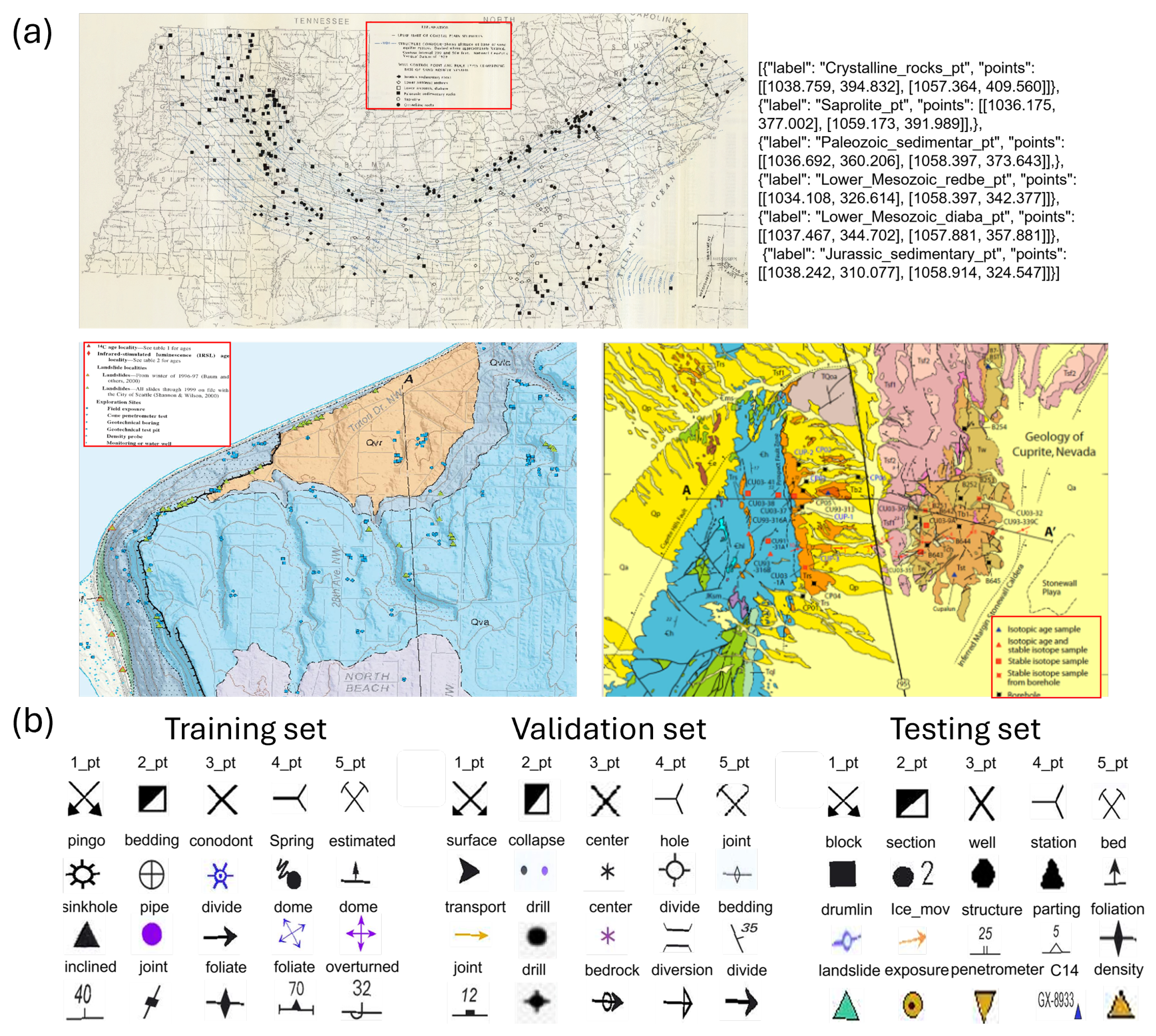
3.5. Point Feature Extraction

Figure 3a illustrates point features in maps with legends marked in red boxes. Notably, the symbols are widely dispersed and represented amidst noisy backgrounds. Figure 3b show the inconsistent symbology of legend items among maps in the training, validation, and testing dataset. While there are consistent symbols across all maps, (first row, “1_pt” to “5_pt”), the same feature type in different scanned documents can be depicted with different symbols or patterns. The cartographic design of the map symbols may change significantly over time, and thus, these symbols appear very differently across maps. To illustrate, symbols like “dome” exhibit significant variations in appearance across different maps in the training dataset. The same holds true for other symbols such as “joint” and “foliate”, where the labels with the same name share some resemblance in the pattern but are largely dissimilar. We began by compiling a collection of the most common point features from our training maps, which contained 48 different legends, including gravel pits, mine shafts, and others.

A straightforward approach to detecting novel classes would involve collecting additional training images for these new classes and incorporating them into the original dataset before retraining or fine-tuning the model. However, this method is inefficient due to the significant costs associated with adequate data collection and model training. To address this, the detection literature has explored generalization from base to novel classes through zero-shot detection, where techniques like prompt-based models [11] were employed to enable the model to recognize new classes without additional training data. Our approach aims to extend the capability of an open-set detector by allowing it to detect the bounding box based on user inputs in the form of an exemplar image. The learning objective is framed as a binary matching problem between input queries (the exemplar images) and the corresponding objects, enabling the model to learn useful correspondences that generalize to unseen queries during testing. A modified YOLO [33] model was adopted for this task. Different from the standard multi-class detection, our input contained the map image and the target point legend image. Specifically, we changed the input channel of YOLOv8 to 6 channels and used the concatenated image of the map and legend as input. For the output, a binary head was applied to predict the target point bounding boxes. Since our task mainly focused on the point position, only the center information of the bounding boxes was maintained for the output raster.

3.6. Evaluation Metrics

The polygon segmentation performance was assessed using widely recognized metrics, including the F1 score, precision, recall, and intersection over union (IoU); the reported mean and median were defined as legend-wise values. The only variation in the evaluation criteria involved weighting the pixels differently. Pixels correctly identified by the color-matching baseline model were labeled as “easy” and the rest as “hard”. In this study, “hard” pixels were weighted at 0.7, while “easy” pixels carried a weight of 0.3. For point detection performance evaluation, instead of merely counting overlapping pixels between the predicted and true maps, we calculated the distance of each pixel in the predicted map to its closest counterpart in the true map, applying a cutoff distance beyond which pixels were not considered valid pairs. Additionally, measures were taken to ensure that each pixel was only counted once. The distances were normalized by the diagonal length of the map, with a value of 0 indicating perfectly overlapping pixels and a value of 1 representing pixels at opposite corners of the map. In this study, we used a cutoff distance of 0.01 to determine valid pairs, and we subsequently calculated the recall, precision, and the F1 score, similar to the approach used for polygon segmentation.

3.7. Workflow Design

The flowchart in Figure 4 illustrates the entire steps of the processing flow, including data preparation, model inference, and postprocessing for the entire map evaluation.

4. Results and Discussion

4.1. Map Unit Extraction

Overall, YOLO represents a robust solution for map unit extraction task. Figure 5a presents visualizations of the extracted map units from patch images, where the training patches are 1024 pixels in size, with a 32-pixel overlap. Figure 5b displays the Precision–Recall (PR) curve across various threshold levels, illustrating the trade-offs between these two metrics. The curve demonstrates that the model excelled in accurately identifying polygon map units while maintaining a low false positive rate. The confusion matrix shown in

Table 1. Normalized confusion matrix of the YOLO model on extracting point, line, and polygon map unit in the legend.

	Pred_Point	Pred_Line	Pred_Polygon	Pred_Background
True_Point	0.36	0.03	0	0.61
True_Line	0	0.73	0	0.27
True_Polygon	0	0	0.91	0.09
True_Background	0.12	0.15	0.74	0

indicates that the YOLO model effectively detected polygon map units, achieving a normalized true positive rate of 0.91. However, despite its strengths, YOLO exhibite some limitations in detecting point and line map units, which are evident in the lower precision scores for these categories. This poor performance on line and point units can largely be attributed to deficiencies in the training data used, such as the distribution of classes, and poor labeling for the true point and line units. To improve the model performance further, efforts are being currently focused on expanding the size of dataset from 150 maps to 3000 maps and making sure maps are fully labeled properly, which aim to achieve a more balanced class distribution and accurate point and line labels for all symbols.

4.2. Polygon Feature Segmentation

4.2.1. Patch and Overlap Size Optimization

We conducted experiments to find the optimal patch and overlap size for the Vanilla U-Net [34] model, as patch size is a crucial hyperparameter that can significantly influence the performance of our model: it affects the context available for learning and can impact both accuracy and computational efficiency. Both the training and validation F1 scores were evaluated, with a focus on validation scores to gauge generalization. To address pixel-level data imbalance, we included only those training patches that contained at least one pixel with a value of 1 (representing polygon features) in the ground truth. As illustrated in

Table 2. Results of experiments with different patch sizes and overlap sizes using the Vanilla U-Net model. All metrics reported here are for “patch-wise” measurement. The parameters with the best performance is in bold.

Model	Patch Size	Overlap	Best Train F1 Score (%)	Best Validation F1 Score (%)	Difference (%)
Vanilla_Unet	128	3	95.29	80.72	14.57
		5	95.89	80.59	15.30
		10	95.49	81.26	14.23
		15	96.05	82.18	13.87
	256	3	90.58	81.65	8.93
		5	91.24	82.26	8.98
		10	92.18	84.23	7.95
		15	93.54	84.39	9.15
		32	94.02	85.72	8.30
	512	3	78.84	75.43	3.41
		5	70.46	69.86	0.60
		10	74.38	72.21	2.17
		15	78.16	72.76	5.40
	1024	3	23.44	20.02	3.42
		5	16.88	15.04	1.84
		10	24.59	26.76	−2.17
		15	24.66	23.53	1.13

, a patch size of 256 with an overlap of 32 yielded the highest validation score of 85.72%, alongside a strong training score of 94.02%. This combination resulted in a modest difference of 8.30% between the training and validation scores, indicating a healthy balance between model fitting and generalization. Notably, increasing the patch size from 128 to 256 consistently improved the validation F1 score, particularly with larger overlaps, suggesting that larger patches help the model capture better contextual information. However, increasing the patch size beyond 256 led to a decline in performance, as seen with patch sizes of 512 and 1024, likely due to the model’s difficulty in handling large patches with insufficient context. These results confirm that a patch size of 256 with an overlap of 32 offers the best balance between model complexity and generalization. This configuration served as the baseline for further comparing different model architectures.

Interestingly, for patch size 128, the best validation F1 score was achieved with an overlap of 15, yielding a score of 82.18%. This suggests that larger overlaps tend to improve results for smaller patch sizes. However, for patch sizes of 512 and 1024, the model consistently underperformed across all overlap values, underscoring the limitations of using larger patches for this specific task.

4.2.2. Model Search and Hyperparameter Tuning

We evaluated three different model architectures—Vanilla U-Net [34], Attention U-Net [35], and MultiRes U-Net [36]—using the optimal patch and overlap configuration from the previous experiments. As shown in

Table 3. Comparison of model architectures using the best patch and overlap size. All metrics reported here are for “patch-wise” measurement. The best one is in bold.

Model	Best Train F1	Best Validation F1
Attention_Unet [35]	92.34%	82.49%
Vanilla_Unet [34]	94.02%	85.72%
MultiRes_Unet [36]	58.93%	56.87%

, the Vanilla U-Net consistently outperformed the others in terms of both its training and validation F1 scores. This suggests that the Vanilla U-Net is better suited for generalization on unseen data. Despite the Attention U-Net’s use of attention mechanisms, it did not surpass the Vanilla U-Net, indicating the added complexity may be unnecessary. The MultiRes U-Net, designed for multi-scale features, underperformed in both its training (58.93%) and validation (56.87%) scores, likely due to overfitting or challenges with our geologic map dataset. Thus, the Vanilla U-Net’s simplicity and strong performance made it the best choice for further experiments and refinements.

Figure 6 displays three challenging scenarios of the model’s segmentation performance across different maps and legends. In each case, the model demonstrated outstanding performance. All three patches showed irregular and discontinuous geometries against noisy backgrounds, with the first one involving both color and pattern matching.

4.2.3. Whole Map Evaluation

We explored various data augmentation techniques to enhance model performance. Since many legends in our dataset rely on color matching, we applied “color jitter” to help the model generalize across different colors. Additionally, we used “random rotation” and “random horizontal and vertical flips” to further improve the generalizability. Data purification was also performed during training: map units with similar colors were combined into a single category to refine the model’s color matching capability. For postprocessing, a mutually exclusive step was used to consolidate multi-class results. For each pixel, the model generated soft logits between 0 and 1 for each legend on the map. In line with standard multi-class segmentation practices, we first selected the highest soft logits value among all classes, and then a threshold was applied to classify predictions as either positive or negative.

We present the overall performance of our proposed methods in terms of the median weighted F1 score on both the validation and testing dataset, as shown in

Table 4. The polygon segmentation performance of prompted U-Net on whole map evaluation. Here, ‘P’ indicates Data Purification, and ‘A’ indicates Strong Data Augmentation.

Methods	Validation				Test
	F1	Precision	Recall	IoU	F1	Precision	Recall	IoU
LOAM [19]	-	-	-	-	80.90	89.10	91.50	-
Prompted U-Net	79.41	84.27	88.40	65.86	90.03	92.76	93.15	82.35
U-Net + P	83.62	87.18	89.77	71.85	90.90	94.21	93.27	83.31
U-Net + P + A	83.71	87.97	89.54	71.98	91.52	94.85	93.01	84.36

. Our approach achieved an F1 score of 91.52%, surpassing the state-of-the-art method by 13.12%. The ablation study included two parts: (1) cleaning the dataset by merging similar map units into a single category to emphasize color matching and (2) applying robust data augmentation techniques, such as color jitter and random horizontal and vertical flips. Both methods significantly improved model performance.

Figure 7 illustrates the model’s performance in polygon feature extraction after aggregating all polygon features across the entire map. Figure 7a displays the raw map visualization, while Figure 7b shows the delineated boundaries of all extracted polygon features, highlighting the model’s capability to accurately identify and represent these features.

This prompt-based segmentation model has several notable limitations. First, the model’s performance is highly dependent on the quality of the prompt image. Issues such as color mismatches, overlapping legends, and noisy backgrounds from scanned, wrinkled maps can significantly impact its effectiveness. Future research should focus on developing techniques to automatically extract high-quality legends from maps. Second, the model struggles to differentiate between legends that are very close to each other. Enhancing localized contrast and improving edge definition in these models could be beneficial.

4.3. Model Performance for Point Detection

Experiments were performed to assess the efficacy of the proposed point detection methods. A set of sample patches is presented here to visually evaluate the model’s performance. Figure 8 demonstrates that the model can accurately detect various types of symbols. Each plot includes the following: (1) a patch image that is cropped from the map, (2) a resized point symbol image from the map unit, (3) a patch image with its predicted result, and (4) a patch image with ground truth annotation. The performance of the model was evaluated by comparing the true label (3) with the predicted label (4), and the majority of these labeled points had very close distances, indicating that the model is capable of accurately extracting symbols. The model performed particularly well in detecting symbols with distinct features, such as prominent edges or contrasting colors.

Table 5. Quantitative evaluation of the proposed point detection models for both the common and rare legend symbols. The threshold for distinguishing between common and rare legend symbols was set at 1000 (the occurrence count of such point symbols in the training dataset).

Methods	Common Legends			Rare Legends
	F1	Precision	Recall	F1	Precision	Recall
Prompted YOLO (Validation)	72.59	82.12	70.59	39.21	32.58	69.46
Prompted YOLO (Testing)	48.10	53.84	80.16	0	0	0

presents a quantitative evaluation of the proposed point detection models for both common and rare legend symbols. The threshold for classifying symbols as common or rare was set at 1000 occurrences in the training dataset. For comparison, the baseline benchmark model, which utilized template matching [34], achieved an F1 score of 0.35 for all point symbols. The performance discrepancy between the validation and testing datasets in Table 5 arose because the testing dataset includes a significantly higher number of unseen point symbols. While the model performed relatively well with sufficient training data, it struggled to generalize to these unfamiliar symbols.

Figure 9 shows the model performance of predicting symbol ‘3_pt’ in a entire map. Compared to the labor-intensive task of manually extracting all point symbols in such a map, the segmentation process for a single type of point symbol using the model for inference was completed within a minute. The model exhibited satisfactory performance in providing a statistical description of the symbols’ distribution, even for maps with lumped symbols that are in close proximity to each other and have a noisy background.

For common point symbols, the model excelled at detecting symbols with distinct characteristics, such as clear boundaries or contrasting colors. The model has been designed with generalizability and robustness in mind, yet we identified situations where the model’s performance was suboptimal. One issue arises when there is a color mismatch between symbols on the map and those in the legend. This misalignment often occurs due to scanning problems such as blurring, aliasing, bleaching, and distortion. Additionally, RGB misalignment, where the red, green, and blue color planes are not properly aligned, can lead to color inconsistencies within the same geographic element. Addressing this challenge requires additional measures. Another issue is the frequent overlap of symbols with linear elements like roads, contour lines, and text. This overlapping can significantly hinder map interpretation, even for human readers, and it is particularly problematic in text recognition within maps with dense and intricate contour lines. To mitigate such issues, sophisticated background removal techniques have been developed. For example, Cao et al. proposed methods for removing solid graphical components and line features, as well as size filtering to separate text from noise [37].

For rare point symbols, the point detection model is constrained by the limited amount of training data. The U-Net model, being a supervised learning model, requires a large amount of labeled data for effective training. However, symbols in scanned documents may appear infrequently in some maps, leading to insufficient data representation. To tackle this issue, one strategy is to explore alternative models that require less data, such as non-learning-based methods like template matching [38] and class-agnostic learning using foundation models as a prior [39,40]. Additionally, it is essential to develop tools that effectively integrate human and machine intelligence at scale [41]. These tools should allow users to quickly (1) review outputs; (2) adjust legend annotations for accurate feature extraction; and (3) correct any imperfections in the extraction process. This approach would enable crowdsourced annotation by non-geoscientists, thereby expanding the dataset for future training. Furthermore, a human-in-the-loop system is under development that allows users to correct the model’s outputs, reducing the annotation time from one week to just a few hours.

5. Conclusions

In this study, we investigated innovative approaches to automatically extract polygon/point features on scanned geologic maps. A modified multi-channel U-Net model, which concatenates map images with an exemplar images from map unit as input, was proposed to enable prompt-based segmentation and detection. The proposed approach was evaluated using various map scenarios, and the experimental results demonstrate its ability to successfully detect various types of symbols while being robust against variations in symbology and map properties. The findings of this study may have practical implications for designing automated models for the faster analysis of geological maps.

This research suggests that current segmentation methods are both applicable and generalizable, though with some trade-offs in performance. Incorporating a “human-in-the-loop” process could further enhance the system, allowing annotators to refine the segmentation and thereby offering room for further improvement. This self-correction process is particularly crucial for edge cases where data are limited, such as with rare point symbols.

For future work, inspired by the recent successes of foundation models, exploring the integration of foundation models like SAM [9] into the current framework could be a promising direction. The advancements of foundation models present the potential to combine pretrained model priors with existing data priors, which could enhance both performance and generalizability. In a human-in-the-loop pipeline, generalizability is critical, as the model needs to produce reliable segmentation results to expedite annotators’ correction tasks. Therefore, the combination of foundation models and human feedback could significantly improve both the speed and accuracy of the segmentation process, leading to more efficient geologic map analysis.

References

1. Thomas, W.A.; Hatcher, R.D. Meeting Challenges with Geologic Maps; American Geological Institute: Alexandria, VA, USA, 2004. [Google Scholar]
2. Soller, D.R.; Berg, T.M. The US national geologic map database project: Overview & progress. In Current Role of Geological Mapping in Geosciences, Proceedings of the NATO Advanced Research Workshop on Innovative Applications of GIS in Geological Cartography, Kazimierz Dolny, Poland, 24–26 November 2003; Springer: Dordrecht, The Netherlands, 2005; pp. 245–277. [Google Scholar]
3. Fortier, S.M.; Hammarstrom, J.; Ryker, S.J.; Day, W.C.; Seal, R.R. USGS critical minerals review. Min. Eng. 2019, 71, 35–47. [Google Scholar]
4. Xu, Y.; Li, Z.; Xie, Z.; Cai, H.; Niu, P.; Liu, H. Mineral prospectivity mapping by deep learning method in Yawan-Daqiao area, Gansu. Ore Geol. Rev. 2021, 138, 104316. [Google Scholar] [CrossRef]
5. Luo, S.; Saxton, A.; Bode, A.; Mazumdar, P.; Kindratenko, V. Critical minerals map feature extraction using deep learning. IEEE Geosci. Remote. Sens. Lett. 2023, 20, 8002005. [Google Scholar] [CrossRef]
6. Budig, B.; van Dijk, T.C. Active learning for classifying template matches in historical maps. In Discovery Science, Proceedings of the 18th International Conference, DS 2015, Banff, Banff, AB, Canada, 4–6 October 2015; Proceedings 18; Springer: Cham, The Netherlands, 2015; pp. 33–47. [Google Scholar]
7. Budig, B.; van Dijk, T.C.; Feitsch, F.; Arteaga, M.G. Polygon consensus: Smart crowdsourcing for extracting building footprints from historical maps. In Proceedings of the 24th ACM SIGSPATIAL International Conference on Advances in Geographic Information Systems, Burlingame, CA, USA, 31 October–3 November 2016; pp. 1–4. [Google Scholar]
8. Soliman, A.; Chen, Y.; Luo, S.; Makharov, R.; Kindratenko, V. Weakly supervised segmentation of buildings in digital elevation models. IEEE Geosci. Remote Sens. Lett. 2022, 19, 7004205. [Google Scholar] [CrossRef]
9. Kirillov, A.; Mintun, E.; Ravi, N.; Mao, H.; Rolland, C.; Gustafson, L.; Xiao, T.; Whitehead, S.; Berg, A.C.; Lo, W.Y.; et al. Segment anything. In Proceedings of the IEEE/CVF International Conference on Computer Vision, Paris, France, 1–6 October 2023; pp. 4015–4026. [Google Scholar]
10. Zou, X.; Yang, J.; Zhang, H.; Li, F.; Li, L.; Wang, J.; Wang, L.; Gao, J.; Lee, Y.J. Segment everything everywhere all at once. In Proceedings of the 37th Conference on Neural Information Processing Systems (NeurIPS 2023), New Orleans, LA, USA, 10–16 December 2023; Volume 36. [Google Scholar]
11. Sun, Y.; Chen, J.; Zhang, S.; Zhang, X.; Chen, Q.; Zhang, G.; Ding, E.; Wang, J.; Li, Z. VRP-SAM: SAM with visual reference prompt. In Proceedings of the IEEE/CVF Conference on Computer Vision and Pattern Recognition, Seattle, WA, USA, 16–22 June 2024; pp. 23565–23574. [Google Scholar]
12. Luo, L.; Li, P.; Yan, X. Deep learning-based building extraction from remote sensing images: A comprehensive review. Energies 2021, 14, 7982. [Google Scholar] [CrossRef]
13. Maxwell, A.E.; Bester, M.S.; Guillen, L.A.; Ramezan, C.A.; Carpinello, D.J.; Fan, Y.; Hartley, F.M.; Maynard, S.M.; Pyron, J.L. Semantic segmentation deep learning for extracting surface mine extents from historic topographic maps. Remote Sens. 2020, 12, 4145. [Google Scholar] [CrossRef]
14. Vasuki, Y.; Holden, E.J.; Kovesi, P.; Micklethwaite, S. An interactive image segmentation method for lithological boundary detection: A rapid mapping tool for geologists. Comput. Geosci. 2017, 100, 27–40. [Google Scholar] [CrossRef]
15. Nunes, I.; Laranjeira, C.; Oliveira, H.; dos Santos, J.A. A systematic review on open-set segmentation. Comput. Graph. 2023, 115, 296–308. [Google Scholar] [CrossRef]
16. Nunes, I.; Pereira, M.B.; Oliveira, H.; dos Santos, J.A.; Poggi, M. Conditional reconstruction for open-set semantic segmentation. In Proceedings of the 2022 IEEE International Conference on Image Processing (ICIP), Bordeaux, France, 16–19 October 2022; pp. 946–950. [Google Scholar]
17. Da Silva, C.C.; Nogueira, K.; Oliveira, H.N.; dos Santos, J.A. Towards open-set semantic segmentation of aerial images. In Proceedings of the 2020 IEEE Latin American GRSS & ISPRS Remote Sensing Conference (LAGIRS), Santiago, Chile, 22–26 March 2020; pp. 16–21. [Google Scholar]
18. Brilhador, A.; Lazzaretti, A.E.; Lopes, H.S. A prototypical metric learning approach for open-set semantic segmentation on remote sensing images. IEEE Trans. Geosci. Remote. Sens. 2024, 62, 5640114. [Google Scholar] [CrossRef]
19. Lin, F.; Knoblock, C.A.; Shbita, B.; Vu, B.; Li, Z.; Chiang, Y.Y. Exploiting Polygon Metadata to Understand Raster Maps-Accurate Polygonal Feature Extraction. In Proceedings of the 31st ACM International Conference on Advances in Geographic Information Systems, New York, NY, USA, 13–16 November 2023; pp. 1–12. [Google Scholar]
20. Lin, T.Y.; Maire, M.; Belongie, S.; Hays, J.; Perona, P.; Ramanan, D.; Dollár, P.; Zitnick, C.L. Microsoft coco: Common objects in context. In Computer Vision—ECCV 2014, Proceedings of the 13th European Conference, Zurich, Switzerland, 6–12 September 2014; Proceedings, Part V 13; Springer: Cham, The Netherlands, 2014; pp. 740–755. [Google Scholar]
21. Uhl, J.H.; Leyk, S.; Chiang, Y.Y.; Duan, W.; Knoblock, C.A. Spatialising uncertainty in image segmentation using weakly supervised convolutional neural networks: A case study from historical map processing. IET Image Process. 2018, 12, 2084–2091. [Google Scholar] [CrossRef]
22. Jiao, C.; Heitzler, M.; Hurni, L. A fast and effective deep learning approach for road extraction from historical maps by automatically generating training data with symbol reconstruction. Int. J. Appl. Earth Obs. Geoinf. 2022, 113, 102980. [Google Scholar] [CrossRef]
23. Minderer, M.; Gritsenko, A.; Stone, A.; Neumann, M.; Weissenborn, D.; Dosovitskiy, A.; Mahendran, A.; Arnab, A.; Dehghani, M.; Shen, Z.; et al. Simple open-vocabulary object detection. In Proceedings of the European Conference on Computer Vision, Tel Aviv, Israel, 23–27 October 2022; Springer: Cham, The Netherlands, 2022; pp. 728–755. [Google Scholar]
24. Kim, H.Y.; De Araújo, S.A. Grayscale template-matching invariant to rotation, scale, translation, brightness and contrast. In Advances in Image and Video Technology, Proceedings of the Second Pacific Rim Symposium, PSIVT 2007, Santiago, Chile, 17–19 December 2007; Proceedings 2; Springer: Berlin/Heidelberg, Germany, 2007; pp. 100–113. [Google Scholar]
25. Korman, S.; Reichman, D.; Tsur, G.; Avidan, S. Fast-match: Fast affine template matching. In Proceedings of the IEEE Conference on Computer Vision and Pattern Recognition, Portland, OR, USA, 23–28 June 2013; pp. 2331–2338. [Google Scholar]
26. Guo, M.; Bei, W.; Huang, Y.; Chen, Z.; Zhao, X. Deep learning framework for geological symbol detection on geological maps. Comput. Geosci. 2021, 157, 104943. [Google Scholar] [CrossRef]
27. Chanda, S.; Prasad, P.K.; Hast, A.; Brun, A.; Martensson, L.; Pal, U. Finding Logo and Seal in Historical Document Images-An Object Detection Based Approach. In Pattern Recognition, Proceedings of the 5th Asian Conference, ACPR 2019, Auckland, New Zealand, 26–29 November 2019; Revised Selected Papers, Part I 5; Springer: Cham, The Netherlands, 2020; pp. 821–834. [Google Scholar]
28. Saeedimoghaddam, M.; Stepinski, T.F. Automatic extraction of road intersection points from USGS historical map series using deep convolutional neural networks. Int. J. Geogr. Inf. Sci. 2020, 34, 947–968. [Google Scholar] [CrossRef]
29. Goldman, M.A.; Rosera, J.M.; Lederer, G.W.; Graham, G.E.; Mishra, A.; Yepremyan, A. Training and Validation Data from the AI for Critical Mineral Assessment Competition; U.S. Geological Survey Sata Release: Reston, VA, USA, 2023. [CrossRef]
30. The HDF Group. Hierarchical Data Format, Version 5. Available online: https://github.com/HDFGroup/hdf5 (accessed on 1 November 2024).
31. Lederer, G.W.; Solano, F.; Coyan, J.A.; Denton, K.M.; Watts, K.E.; Mercer, C.N.; Bickerstaff, D.P.; Granitto, M. Tungsten skarn mineral resource assessment of the Great Basin region of western Nevada and eastern California. J. Geochem. Explor. 2021, 223, 106712. [Google Scholar] [CrossRef]
32. Glen, J.; Earney, T. GeoDAWN: Airborne Magnetic and Radiometric Surveys of the Northwestern Great Basin, Nevada and California; U.S. Geological Survey: Reston, VA, USA, 2024.
33. Redmon, J.; Divvala, S.; Girshick, R.; Farhadi, A. You only look once: Unified, real-time object detection. In Proceedings of the IEEE Conference on Computer Vision and Pattern Recognition, Las Vegas, NV, USA, 27–30 June 2016; pp. 779–788. [Google Scholar]
34. Ronneberger, O.; Fischer, P.; Brox, T. U-net: Convolutional networks for biomedical image segmentation. In Medical Image Computing and Computer-Assisted Intervention—MICCAI 2015, Proceedings of the 18th International Conference, Munich, Germany, 5–9 October 2015; Proceedings, Part III 18; Springer: Cham, The Netherlands, 2015; pp. 234–241. [Google Scholar]
35. Xu, Z.; Wang, S.; Stanislawski, L.V.; Jiang, Z.; Jaroenchai, N.; Sainju, A.M.; Shavers, E.; Usery, E.L.; Chen, L.; Li, Z.; et al. An attention U-Net model for detection of fine-scale hydrologic streamlines. Environ. Model. Softw. 2021, 140, 104992. [Google Scholar] [CrossRef]
36. Ibtehaz, N.; Rahman, M.S. MultiResUNet: Rethinking the U-Net architecture for multimodal biomedical image segmentation. Neural Netw. 2020, 121, 74–87. [Google Scholar] [CrossRef]
37. Cao, R.; Tan, C.L. Separation of overlapping text from graphics. In Proceedings of the Sixth International Conference on Document Analysis and Recognition, Seattle, WA, USA, 13 September 2001; pp. 44–48. [Google Scholar]
38. Qiu, Q.; Tan, Y.; Ma, K.; Tian, M.; Xie, Z.; Tao, L. Geological symbol recognition on geological map using convolutional recurrent neural network with augmented data. Ore Geol. Rev. 2023, 153, 105262. [Google Scholar] [CrossRef]
39. Bharadwaj, R.; Naseer, M.; Khan, S.; Khan, F.S. Enhancing Novel Object Detection via Cooperative Foundational Models. arXiv 2023, arXiv:2311.12068. [Google Scholar]
40. Pan, H.; Yi, S.; Yang, S.; Qi, L.; Hu, B.; Xu, Y.; Yang, Y. The Solution for CVPR2024 Foundational Few-Shot Object Detection Challenge. arXiv 2024, arXiv:2406.12225. [Google Scholar]
41. Russakovsky, O.; Li, L.J.; Fei-Fei, L. Best of both worlds: Human-machine collaboration for object annotation. In Proceedings of the IEEE Conference on Computer Vision and Pattern Recognition, Boston, MA, USA, 7–12 June 2015; pp. 2121–2131. [Google Scholar]
42. DARPA. Critical Mineral Assessments with AI Support (CriticalMAAS). Available online: https://shorturl.at/Tgacn (accessed on 1 November 2024).
43. DARPA. Critical Mineral Assessments with AI Support (CriticalMAAS). Available online: https://shorturl.at/MlhnK (accessed on 1 November 2024).
Figure 1. Example of data visualization: This figure illustrates a sample dataset embedded within a comprehensive map. It includes the following components: 1. Main Map Content: Displays the area containing key features of interest. 2. Corner Coordinate: Typically located at the corner of the map content for georeferencing purposes. 3. Text Information: Provides metadata such as map location and geological age. 4. Map Legend Area: Contains a list of map units along with their descriptive text. 5. Segmentation Map: Shows an example of extracted polygon features using the map unit “Qal” as the query key.
Geosciences 14 00305 g001
Figure 2. (a) A geologic map sample with the map content area and legend area highlighted in red. The original map is overlaid with polygonal features to emphasize the discontinuity and the varying shapes and sizes of these features. (b) An illustration of the patch-wise segmentation model using map unit as the prompt. (c) Congregated results after the patch-wise segmentation model inference and restitching.
Geosciences 14 00305 g002
Figure 3. (a) The uppermost plot depicts a geologic map featuring a legend with six symbol items, which are displayed as a red box in the upper-middle region; these symbols are almost indistinguishable when lumped together. The accompanying JSON file on the right-hand side documents the names and coordinates of each legend item. The bottom section showcases two additional maps with legends marked in red boxes. (b) The inconsistent symbology of legend items among maps in the training, validation, and testing dataset.
Geosciences 14 00305 g003
Figure 4. Flowchart illustrates the entire steps of the processing flow.
Geosciences 14 00305 g004
Figure 5. Model performance on legend map unit extraction. (a) Visualization of the extracted map unit on patch images. (b) Precision–Recall curve to illustrate the trade-off between precision and recall for different thresholds.
Geosciences 14 00305 g005
Figure 6. (ac) Model performance on example patched image. This visualization includes patch image, legend, predicted segmentation mask, and ground truth (GT) segmentation mask.
Geosciences 14 00305 g006
Figure 7. Model performance on polygon feature extraction after aggregating all polygon and point features across the entire map. (a) Visualization of the raw map; (b) visualization of the extracted features; (c,d) zoom-in plot for better visualization. Different colors represents different point features.
Geosciences 14 00305 g007
Figure 8. (a,b) The model’s performance in validation data for various types of legend items. The columns from left to right are (1) patchified image, (2) resized legend item, (3) model predicted annotation (red circle) (4) ground truth annotation (blue circle).
Geosciences 14 00305 g008
Figure 9. Model performance on an entire map; red circle represents the model prediction, and blue circle represents the ground truth. (a) Model performance for predicting symbol ’3_pt’, (b) zoom-in plot for better visualization.
Geosciences 14 00305 g009