Earthquake Damage Susceptibility Analysis in Barapani Shear Zone Using InSAR, Geological, and Geophysical Data

Abstract

The identification of areas that are susceptible to damage due to earthquakes is of utmost importance in tectonically active regions like Northeast India. This may provide valuable inputs for seismic hazard analysis; however, it poses significant challenges. The present study emphasized the integration of Interferometric Synthetic Aperture Radar (InSAR) deformation rates with conventional geological and geophysical data to investigate earthquake damage susceptibility in the Barapani Shear Zone (BSZ) region of Northeast India. We used MintPy v1.5.1 (Miami INsar Timeseries software in PYthon) on the OpenSARLab platform to derive time series deformation using the Small Baseline Subset (SBAS) technique. We integrated geology, geomorphology, gravity, magnetic field, lineament density, slope, and historical earthquake records with InSAR deformation rates to derive earthquake damage susceptibility using the weighted overlay analysis technique. InSAR time series analysis revealed distinct patterns of ground deformation across the Barapani Shear Zone, with higher rates in the northern part and lower rates in the southern part. The deformation values ranged from 6 mm/yr to about 18 mm/yr in BSZ. Earthquake damage susceptibility mapping identified areas that are prone to damage in the event of earthquakes. The analysis indicated that about 46.4%, 51.2%, and 2.4% of the area were low, medium, and high-susceptibility zones for earthquake damage zone. The InSAR velocity rates were validated with Global Positioning System (GPS) velocity in the region, which indicated a good correlation (R² = 0.921; ANOVA p-value = 0.515). Additionally, a field survey in the region suggested evidence of intense deformation in the highly susceptible earthquake damage zone. This integrated approach enhances our scientific understanding of regional tectonic dynamics, mitigating earthquake risks and enhancing community resilience.

1. Introduction

Shear zones are regions of concentrated deformation within the Earth’s crust, where differential stress leads to localized strain and displacement of rock masses. These zones vary significantly in width and exhibit complex deformation patterns, encompassing brittle fracturing in the upper crust and ductile flow at deeper levels, driven by differential stress, thermal gradients, and fluid interactions [1,2]. Brittle shear zones are characterized by faulting and fracturing that produce fine-grained cataclasite, while ductile shear zones form mylonites with notable foliation, lineation, and folding due to plastic flow [3,4,5]. These deformation zones are critical for understanding regional tectonic dynamics, including earthquake activity and associated risks in active regions like Northeast India.

Among the advancements in observing crustal deformation, Synthetic Aperture Radar Interferometry (InSAR) has emerged as a powerful tool to measure subtle ground movements accurately, offering new insights into seismic, volcanic, and subsidence phenomena. Initially demonstrated in topographic mapping, InSAR gained attention in seismic research following its application to the 1992 Landers earthquake, where it mapped deformation over large areas through the Differential InSAR (DInSAR) technique pioneered by Massonnet et al. [6]. This success catalyzed the development of Differential InSAR (DInSAR), which allowed precise tracking of surface deformation events but encountered decorrelation issues, especially in areas with substantial vegetation or atmospheric disturbances [7,8].

To enhance accuracy in challenging terrains, Persistent Scatterer Interferometry (PSInSAR) was developed, focusing on stable, reflective ground points such as buildings or exposed rock surfaces, facilitating millimeter-scale monitoring even in urban areas [9]. This technique allows for the millimeter-scale detection of ground deformation, making it particularly valuable in densely built urban areas where stable targets are abundant [9,10]. PSInSAR has proven instrumental in urban deformation studies, offering enhanced temporal resolution and accuracy in tracking subtle subsidence and structural shifts over time. However, for regions lacking sufficient stable scatterers, especially in rural or natural settings, the Small Baseline Subset (SBAS) method was introduced as a complementary InSAR technique. SBAS achieves reliable deformation measurements by selecting image pairs with minimal temporal and spatial baselines, thus reducing atmospheric and decorrelation noise [11]. This approach has broadened the applicability of InSAR, enabling effective monitoring across diverse geohazards, including landslides, volcanic activity, and infrastructure stability [12,13]. SBAS has notably expanded the role of InSAR in monitoring areas like Mexico City, where subsidence due to groundwater extraction poses a significant risk to infrastructure [14,15]. These advancements underscore the capability of InSAR as a powerful remote sensing tool capable of detecting surface deformations down to millimeter accuracy. Such deformations, often precursors to seismic events, provide crucial insights into tectonic stresses and potential fault slip areas [16,17,18].

The growing availability of high-resolution satellite data from platforms like Sentinel-1 and Advanced Land Observing Satellite-2 (ALOS-2) has further enhanced the spatial and temporal precision of InSAR techniques, facilitating continuous monitoring of geohazards. Advanced corrections for atmospheric and ionospheric effects have improved data quality, with multi-temporal InSAR analysis increasingly employed in seismic and deformation studies [19,20]. Emerging approaches integrate machine learning for automated deformation detection, augmenting InSAR’s utility in real-time geohazard assessment [21,22,23]. Additionally, integrating InSAR with geophysical and geological data models enhances understanding of subsurface dynamics, including fault structures and lithospheric stress, underscoring its potential in seismic hazard analysis [24,25].

The Barapani Shear Zone (BSZ) in Meghalaya represents a significant knowledge gap in InSAR-based research. Despite the advantages of InSAR, the BSZ’s tectonic behavior has not been extensively studied using this high-precision method, limiting understanding of the region’s deformation characteristics and seismic susceptibility. This study addresses this gap by integrating InSAR-derived deformation rates with geological and geophysical data, including gravity and magnetic anomalies, to evaluate earthquake damage susceptibility in the BSZ. Such a comprehensive approach not only facilitates accurate identification of deformation-prone areas but also supports improved seismic risk assessment, enabling better preparedness and risk mitigation strategies in this tectonically active region.

2. Geology and Tectonics of Barapani Shear Zone (BSZ)

The Barapani Shear Zone (BSZ), a prominent NE–SW trending geological feature within the Shillong Plateau in Meghalaya, India, reveals an intricate interplay of lithological and structural complexities within the Precambrian gneissic complexes of the Indian Shield. Geographically centered around 25.57° N and 91.88° E, the study area spans approximately 1444.53 km² and is bounded by a 10 km buffer from the BSZ’s center line (Figure 1), covering regions within the Shillong Group’s Precambrian phyllites. These phyllites exhibit high fracture density, complex structural features, and multiple deformation phases, characteristic of an active tectonic setting [26].

The geological makeup of the BSZ includes highly deformed subvertical beds and a suite of intrusive rocks, such as meta-gabbro/dolerite and granite plutons, including Mylliem, South Khasi, Kyrdem, and Nongpoh granites, which add to the structural complexity [27]. This area’s tectonic activity is evidenced by prominent mylonitic foliation, elongated and flattened quartz and feldspar, and clear indications of grain-size reduction due to shearing processes [28]. Geographically, the BSZ extends from Umroi in the northeast to Tyrsad in the southwest, primarily following the Umiam River’s path (Figure 1). Geomorphic evidence of left-lateral slip includes features such as elongated ridges that show southwest-directed dragging effects attributed to significant tectonic movement. Notably, the BSZ has influenced regional geomorphology, forming depressions like the Barapani reservoir, which is hypothesized to result from minor tilting related to fault dynamics. Additionally, indicators of dextral shear, such as quartz vein gash openings and well-formed pebble lineation within conglomerates, further highlight the area’s tectonic activity [26,29]. Structural features within the BSZ, including foliation, lineation, asymmetric folds, and deformation bands, align in the NE–SW direction, underscoring the intense deformation regime prevalent in this shear zone. The zone’s complex structural and lithological attributes make it a key area for understanding crustal dynamics within the Shillong Plateau.

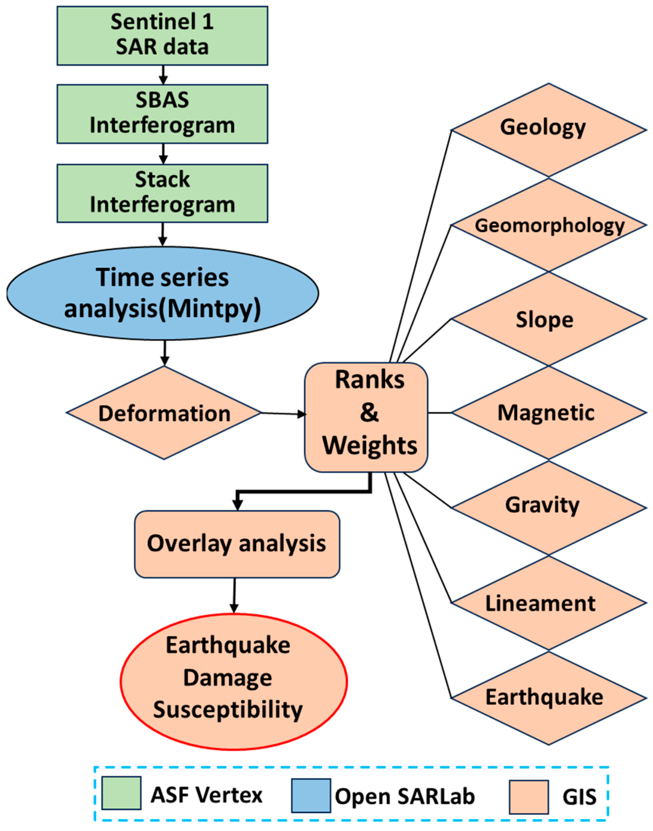
3. Data and Methodology

3.1. Data Utilized

The primary dataset utilized was the Sentinel-1 SAR data, which served as the backbone for analyzing ground deformation through InSAR techniques. A total of 220 interferogram pairs were acquired from the Alaska Satellite Facility (ASF) Vertex platform, covering a significant observation period from 14 March 2017 to 24 May 2024. The SAR data were collected in Interferometric Wide (IW) mode, path 41, frame 80, in ascending mode with VV + VH polarization. In present study, data from only ascending track was considered, as the study region lacks data coverage of good coherence from descending track. In addition to SAR data, comprehensive geological and geophysical data products were collected from Geological Survey of India (GSI). These include geology, geomorphology, gravity, and magnetic data products. Lineament density map was prepared with combination of Shuttle Radar Topography Mission (SRTM) and Linear Imaging Self-Scanning Sensor-IV (LISS-IV) satellite data. Historical earthquake records were acquired from the National Centre for Seismology (NCS).

3.2. InSAR Time Series Analysis

The Small Baseline Subset (SBAS) approach, as proposed by Berardino et al. [11], was utilized in this study to produce coherent interferograms and extract time series deformation. The SBAS technique is particularly effective in minimizing spatial and temporal decorrelation, which can degrade the quality of interferometric measurements. It uses a set of linear equations to establish a relationship between observed phase differences and surface displacements over time [11,30]. Following the generation of coherent interferograms, OpenSARLab platform was utilized for time series analysis [31,32,33,34,35,36]. By leveraging predefined notebooks within the OpenSARLab platform, we prepared the data for subsequent analysis in MintPy (Miami INsar Time series software in PYthon). MintPy employs a system of equations to minimize the residuals between the observed and modeled phase measurements. This is accomplished through a least-squares adjustment process [30,37].

SAR image coregistration was performed using the GAMMA software integrated into the OpenSARLab pipeline, ensuring sub-pixel accuracy and high-quality interferograms. To enhance the signal-to-noise ratio and computational efficiency, a multilooking ratio of 4:1 (range:azimuth) was applied during interferogram generation. The Goldstein phase filter was employed to suppress noise while retaining key deformation signals, and the SBAS method, as implemented in MintPy, was used to generate a time series of ground deformation. This included the use of a network unwrapping algorithm to ensure phase continuity and coherence. To mitigate atmospheric artifacts, ERA5 weather model data was incorporated for phase delay correction in MintPy’s atmospheric filter module, addressing both tropospheric and ionospheric delays. Unwrapping errors were minimized using the Statistical-cost Network-flow Algorithm for Phase Unwrapping (SNAPHU) integrated within the MintPy pipeline, which was tuned with optimized coherence thresholds (0.6) to address errors in low-coherence regions typical of vegetated or rugged terrains.

The time series data derived from this analysis were validated using limited published GPS velocity data, ensuring that the InSAR measurements maintained consistency and reliability. This validation process involves transforming the 3D GPS velocity components into a line-of-sight direction using the GPS LOS velocity validation equation [36,37,38], as given in Equation (1):

Gl = −VEcos(ϕ)sin(θ) + VNsin(ϕ)sin(θ) + VUcos(θ)

(1)

where Gl is the GPS LOS velocity, VE is the velocity component in the east, VN is the velocity component in the north, and VU is the velocity component in the up direction. Here, ϕ represents the azimuth heading angle, and θ is the incidence angle. This ensures a precise transformation of the data, maintaining consistency and reliability across different measurement techniques. Additionally, a one-way Analysis of Variance (ANOVA) test was conducted to evaluate the variance between the average velocities of GPS and InSAR measurements to further enhance the results.

3.3. Weighted Overlay Analysis

The earthquake damage susceptibility zones were identified through overlay analysis with InSAR velocity map as primary input. In addition to InSAR, seven additional parameters were considered, including three parameters derived in the present study such as lineament, slope, and earthquake. Lineament map was prepared from 5.8 m spatial resolution LISS-IV Indian satellite data through visual interpretation techniques followed by field visits. Slope map was prepared using Digital Elevation Model (DEM) data from SRTM [39] using terrain analysis in ArcGIS. Past earthquakes for the duration 2012–2023 were obtained from National Centre for Seismology (NCS) [40] to prepare earthquake map of the BSZ. In addition, geological and geophysical data products such as geology, geomorphology, gravity, and magnetic data were obtained from Geological Survey of India (GSI). These data are freely available in public domain [41] after necessary corrections by the competent authority of GSI. Each parameter contributes differently to earthquake damage susceptibility, and hence, we assigned weights and ranks to each parameter based on the understanding of their influence on earthquake damage susceptibility. All 8 parameters were combined, and weighted overlay analysis as derived from AHP [42] was carried out to generate the earthquake damage susceptibility map [43,44].

$$S={\displaystyle {\sum }_{i=1}^n}{w}_i\times x_i$$

(2)

where S is the Earthquake Damage Susceptibility Index, representing the combined influence of all parameters. $w_i$ is the weight assigned to parameter i, $x_i$ is the standardized or normalized value (rank) of parameter i, and n is the total number of parameters considered (in this case, 8 parameters). Ranks and Weights of each parameter were assigned based on its relative importance in view of causing damage in the event of earthquake, expert knowledge, field knowledge, and equal distribution of values in considered parameter [45,46]. Figure 2 represents the work flow adopted in present study.

4. Results and Discussion

This analysis focused on deformation and earthquake damage susceptibility with primary inputs from InSAR and additional inputs from geological and geophysical parameters.

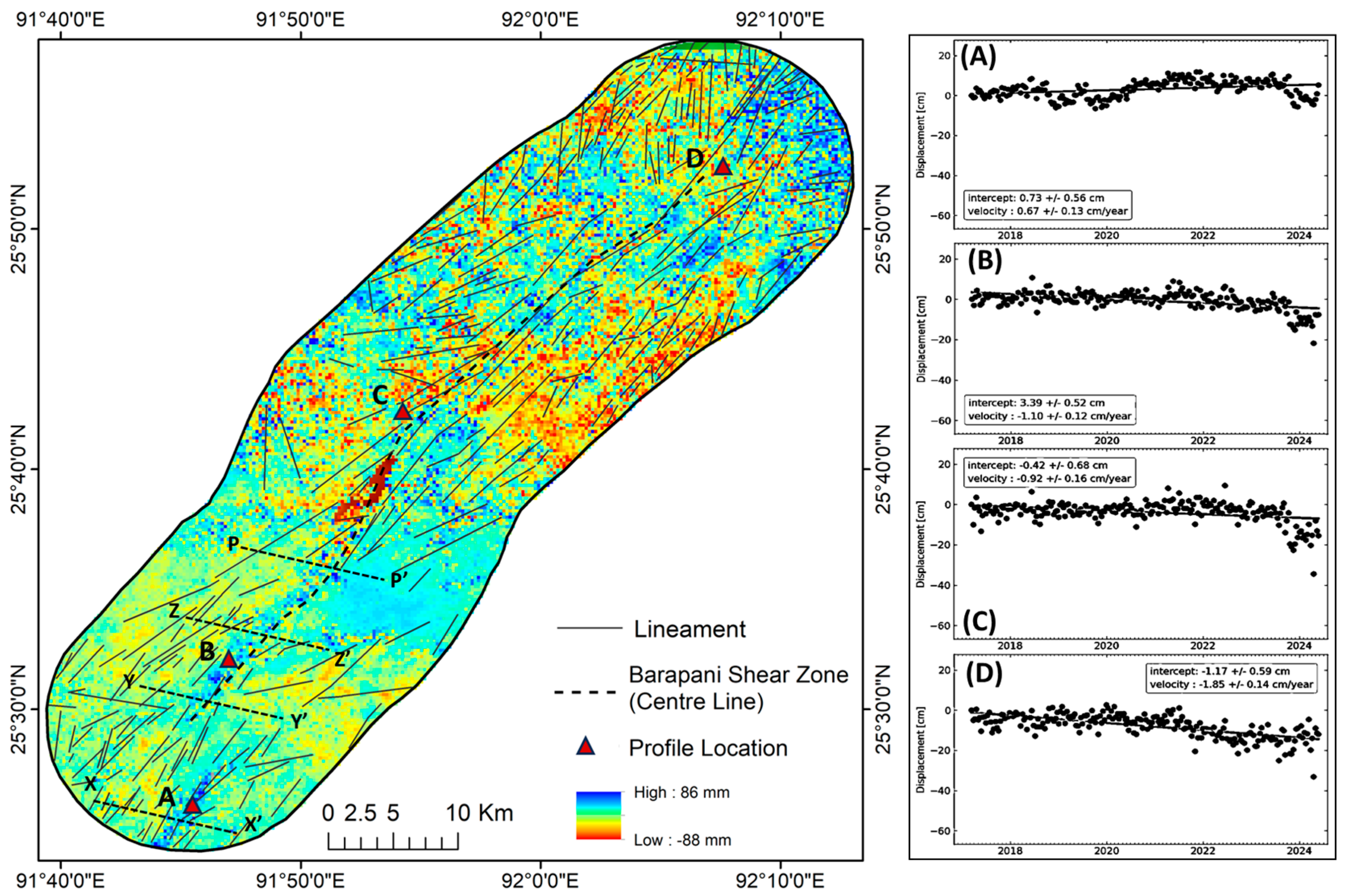
4.1. InSAR-Based Time Series Analysis

Time series data from Sentinel-1 SAR provided detailed insights into the deformation rates in the shear zone. The deformation rates within the BSZ vary significantly, ranging from 6 mm/year to nearly 18 mm/year. This variation in deformation rates is indicative of the dynamic and active tectonic processes occurring within the shear zone. In the southern part of the BSZ, the deformation rates are relatively lower, starting at approximately 6 mm/year. As we move northward, the deformation rates increase substantially, reaching up to 18 mm/year. This significant rise in deformation rates suggests a higher level of tectonic activity and stress accumulation in the northern section. The northern part of the BSZ is likely experiencing more intense shear movements, which could be associated with the interactions between different fault segments and the broader regional tectonic forces. In order to retain only the deformation component due to tectonics, we selected a scatterer with a coherence value of >0.6 for InSAR time series analysis, thereby maintaining accuracy in the measurements. Additionally, we incorporated statistical analysis to validate the InSAR deformation rates, as described in Section 5.

Figure 3 illustrates the deformation rate changes over time, providing a clear visual representation of the gradual increase in rates from 2017 to 2024. Each dot in Figure 3A–D describes the position of an object on the ground, and the intercept (often a constant) can be related to velocity when these positions change over time. An intercept in position data typically refers to the value of position at t = 0 (in this case), or it could be the starting position in the case of a constant velocity scenario. Since, in this case, the position data follow a linear trend (i.e., the position changes uniformly over time), the slope of the position–time curve will directly provide the velocity. Therefore, the intercept represents the initial position, whereas velocity was derived from the slope of the position–time curve. The locations A, B, C, and D were selected parallel to the BSZ center line in order to estimate deformation changes near BSZ with time. These locations were selected based on stable sites devoid of human settlement and anthropogenic activities after field visits in the study area. An example field photo is shown in Section 4.2. The identified deformation rates within the BSZ have important implications for seismic hazard assessment and risk mitigation. The higher deformation rates in the northern part of the BSZ suggest a region of increased seismic risk, where significant tectonic stress is being accumulated. Understanding these deformation patterns is crucial for mapping damage-susceptible zones due to earthquakes and, hence, implementing effective preparedness strategies. Although deformation rates are comparatively less in the southern portion, they are more prominent near the BSZ center line. Profiling across the BSZ was conducted to further investigate the deformation characteristics of the region. Figure 4 illustrates the deformation rates across a few segments of the shear zone at locations marked in Figure 3 (Locations X–X′, Y–Y′, Z–Z′ and P–P′). Significant spikes in deformation rates are observed within the BSZ line, indicating localized areas of increased tectonic activity near the shear zone. The deformation rates on both flanks away from the BSZ are lesser than in the shear zone region. The offsets in deformation rates (about 4mm/yr in most cases) observed in the profiles indicate localized deformation in the shear zone. These localized deformations are clearly visible and may be useful in tracing the fault line, as indicated by Figure 3. In order to confirm the correctness of these visual observations of spikes in deformation rates, we validated observed InSAR velocity with the GPS velocities in selected regions. Additionally, we performed a one-way Analysis of Variance (ANOVA) test to evaluate the variance between the average velocities of the groups (GPS and InSAR) to further enhance the results, as described in Section 5.

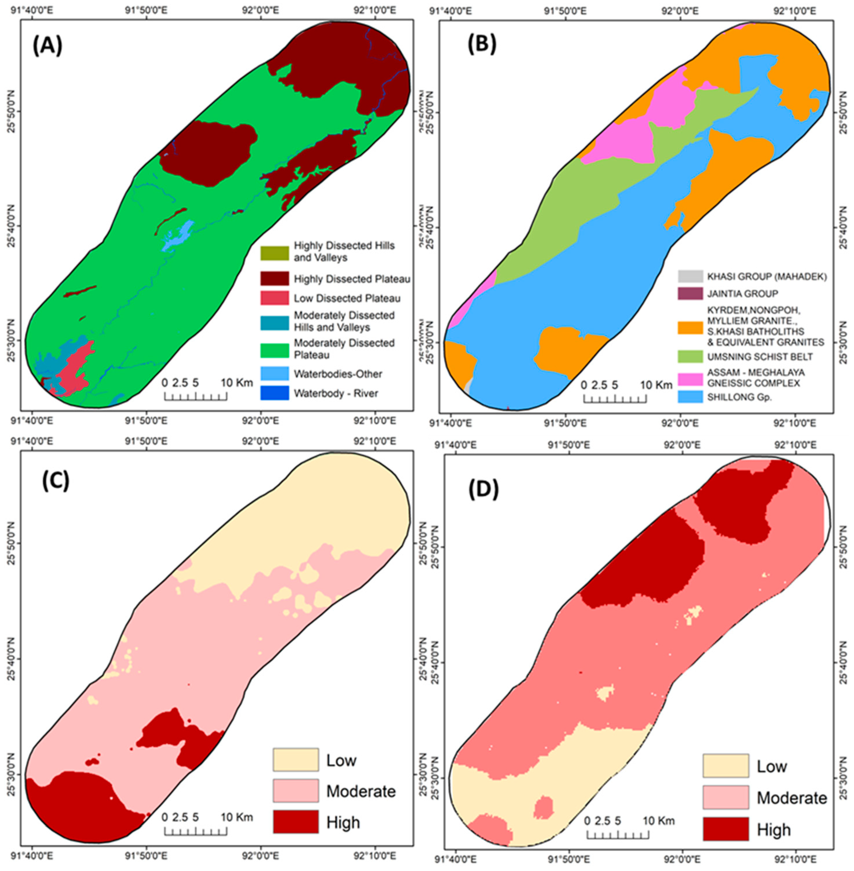
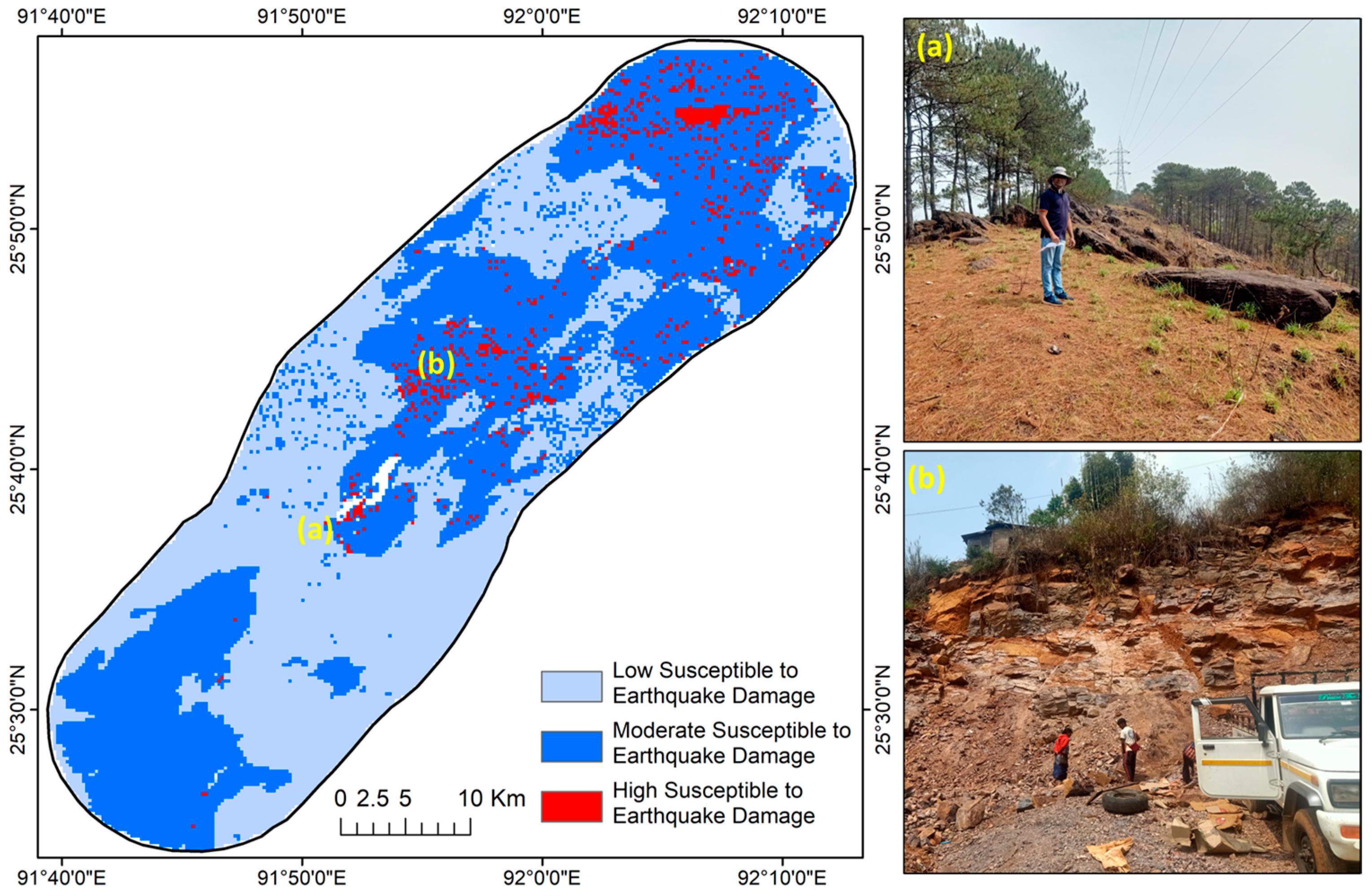
4.2. Data Integration and Earthquake Damage Susceptibility Mapping

The integration of geological and geophysical data was essential to understanding the factors contributing to earthquake damage susceptibility in the BSZ. By combining multiple datasets, we captured the intricate interplay between tectonic structures, subsurface conditions, and surface deformation, providing a holistic perspective on the region’s seismic risks.

The cumulative deformation map (2017 and 2024) illustrates that the BSZ experiences significantly higher deformation rates compared with the surrounding areas. The lineament map shows a bimodal pattern with high density along the BSZ center line and is primarily oriented in the NE–SW direction (Figure 1 and Figure 5D). The slope gradients across the BSZ indicated a steeper slope near the shear zone (Figure 5B). This information is crucial for evaluating terrain stability, identifying potential earthquake-prone areas, and further elucidating the geological dynamics of the BSZ. Past earthquake events from 2012 to 2023 show the spatial and temporal patterns of seismic events, providing insights into the earthquake-prone areas surrounding the BSZ. The previous earthquake map shows that past high-magnitude earthquakes have occurred at the northeastern and southwestern tips of the study area (Figure 5C).

In addition, the geological and geophysical data products obtained from the Geological Survey of India (GSI), as shown in Figure 6, were vital for identifying zones with varying rock strengths and susceptibilities to seismic shaking. Areas with softer lithologies or faulted zones are more prone to ground deformation and can amplify seismic waves, increasing vulnerability to earthquake damage. The geomorphological data products provided surface features and landforms that influence ground shaking during earthquakes. Incorporating gravity and magnetic field data further enhanced our understanding of subsurface structures in the Barapani Shear Zone. Gravity anomalies provide variations in subsurface density, which may reveal the presence of faults or fractures affecting seismic wave propagation. Magnetic field data highlighted distributions of magnetic minerals associated with tectonic activity, helping to identify areas of stress accumulation. By integrating these diverse datasets, we conducted a comprehensive analysis that captured the multi-faceted nature of earthquake damage susceptibility.

Each parameter contributes differently to earthquake damage susceptibility, and their combined effect provides a comprehensive assessment of potential seismic hazards. Deformation values have a direct relationship with tectonic activity and fault movement, and areas having high deformation (both upliftment and subsidence) may contribute more toward damage in the event of an earthquake. Therefore, we assigned high values to deformation >30mm/yr (upliftment) and <−30 mm/yr (subsidence) with field knowledge that the average velocity in the region is around 30 mm/yr, as given by Mukul et al. [47], and total range of values −30 to >30 can be grouped into three equal classes. Therefore, deformation rates and lineaments were given higher weights due to their direct relationship with expected damage. Conversely, parameters like geology and geomorphology, while still important, were assigned slightly lower weights. Slope data can highlight areas prone to damage by seismic events, while previous earthquake occurrences provide historical context to the seismic activity. Gravity and magnetic anomalies help delineate subsurface structures that could influence seismic behavior. The specific weights and ranks assigned to each parameter were meticulously determined and are provided in

Table 1. Weights and ranks assigned to parameters influencing earthquake damage susceptibility based on their impact on seismic hazards.

Parameter Derived in Present Study	Weight	Rank	Parameter Obtained from GSI Data Products	Weight	Rank
InSAR Velocity (mm/yr) Low (>−30) Medium (−30 to 30) High (>30 mm/yr)	30	9 5 9	Geology Assam–Meghalaya Gneissic Complex Jaintia Gp. Khasi Gp. (Mahadek Fm.) Kyrdem, Nongpoh, Mylliem Granite., S.Khasi Batholiths and Equivalent Granites Shillong Gp. Umsning Schist Belt Gr.	10	2 5 8 3 9 7
Lineation Density Low (60) Medium (120) High (180)	20	4 7 9	Geomorphology Highly Dissected Hills and Valleys Highly Dissected Plateau Low Dissected Plateau Moderately Dissected Hills and Valleys Moderately Dissected Plateau Waterbodies—Other Waterbody—River	10	8 7 5 6 5 3 3 -
Slope (Degree) Low (0–30) Medium (30–45) High (45–90)	10	3 5 9	Gravity (mGal) Low (−52–40) Medium (−40–−25) High (−25–−10)	5	9 5 2
Earthquakes (Mw) Low (2.2–2.8) Medium (2.8–3.4) High (3.4–4)	10	3 6 9	Magnetic (nT) Low (−479–−133) Medium (−133–214) High (>214)	5	5 3 2

.

The resulting earthquake susceptibility map, generated from weighted overlay analysis, indicates varying damage susceptibility, from low to high, based on the integrated analysis of all the contributing parameters. The earthquake damage susceptibility map reveals that the center of the BSZ and certain patches toward the northeastern tip exhibit a very high susceptibility to earthquake damage. Most of the areas with low susceptibility are found in the western part of the region. Zones with moderate and high susceptibility are scattered in patches across the entire study area, as shown in Figure 7. This map is a vital tool for disaster preparedness and risk mitigation, enabling targeted efforts to strengthen infrastructure and enhance community resilience in the most vulnerable areas. Field surveys in a few selected regions revealed that highly vulnerable areas fall under high deformation and structurally disturbed areas (Figure 7b). Location (a) is on top of the exposed BSZ and devoid of structural disturbance observed during the field survey, as shown in the field photograph (Figure 7). However, location (b) is one of the examples where evidence of intense deformation was observed during the field survey, which falls under the highly susceptible earthquake damage zone. Some regions in the central and northern parts are highly vulnerable to earthquake damage. About 2.5% of the area falls under the category of highly vulnerable to earthquake damage.

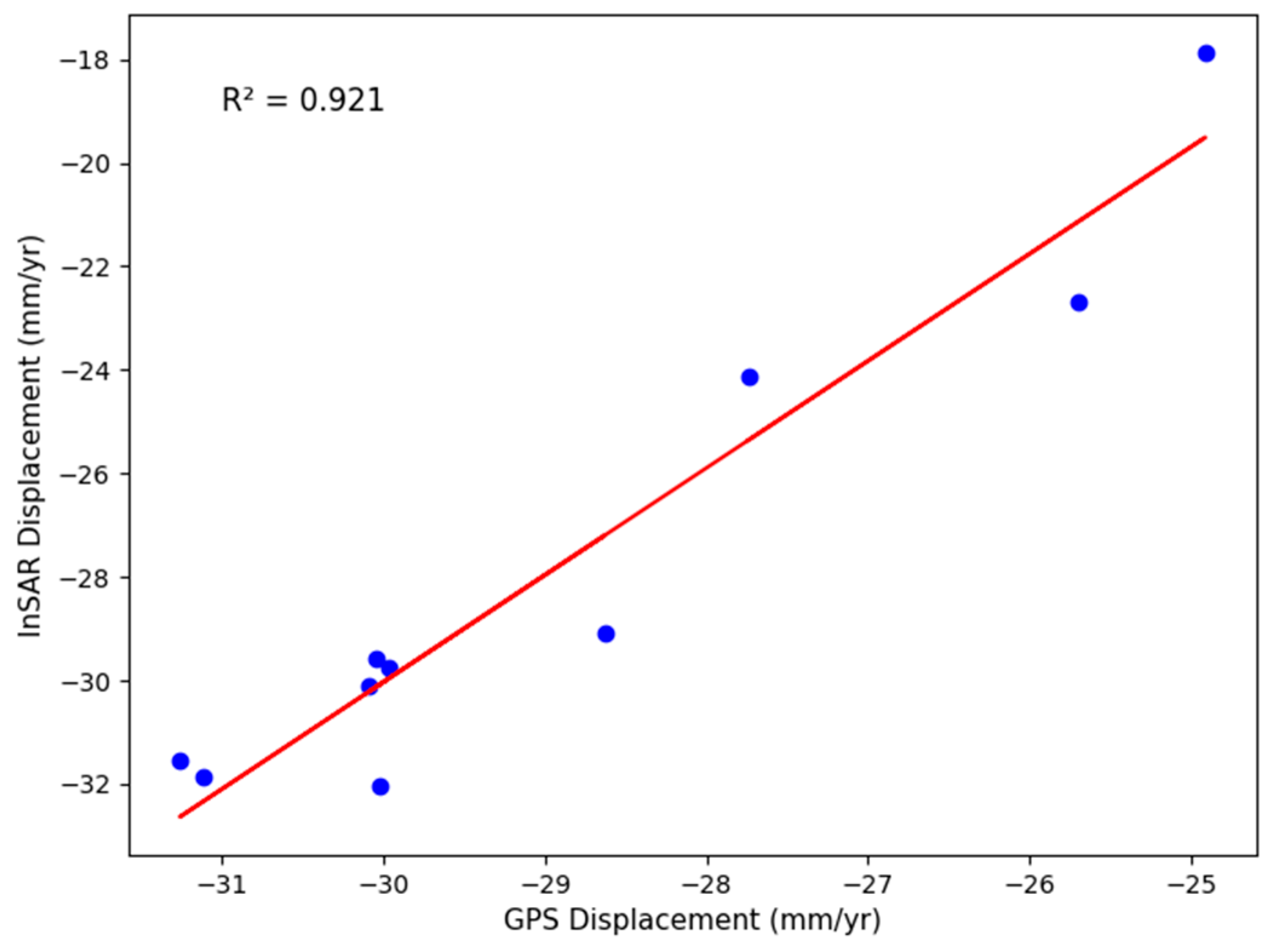
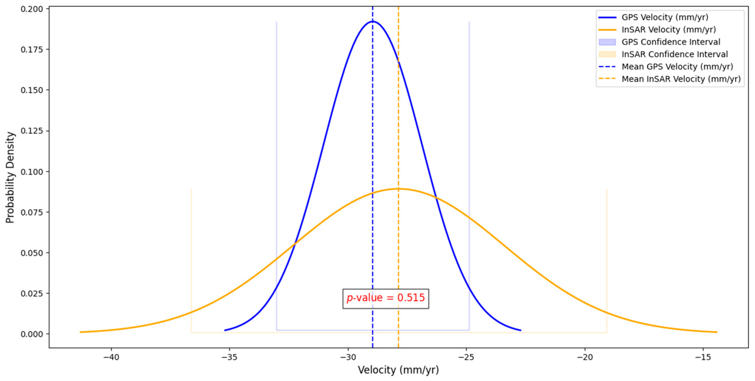
5. Validation of InSAR Velocity Rates

As InSAR Line-of-Sight (LOS) velocity was one of the most important parameters in the present analysis, we validated the InSAR LOS velocity by comparison with the published Global Positioning System (GPS) velocity in a few locations in and around the study area. For this comparison, GPS velocities from 10 GPS stations located in Northeast India were selected and converted into LOS velocities. We extracted InSAR velocity points close to each GPS station for the comparative study, as shown in

Table 2. InSAR and GPS_LOS velocities in a few selected regions in Northeast India (GPS velocity taken from [47,48,49]).

S. No.	Station Name	Location	ITRF08 (mm/Year)		GPSLOS (mm/Year)	InSAR (mm/Year)
			VE	VN
1	NONG	Nongpoh, Meghalaya	39.33 ± 0.28	29.86 ± 0.28	−27.75	−24.11
2	SHIL	Shillong, Meghalaya	35.80 ± 0.80	30.50 ± 0.50	−25.70	−22.68
3	MOPE	Mopen, Meghalaya	37.20 ± 0.80	30.70 ± 0.60	−24.91	−17.87
4	SOKR	Sokra Pam, Assam	38.94 ± 0.91	27.51 ± 0.9	−30.05	−29.56
5	PANI	Panimura, Assam	38.07 ± 0.46	29.19 ± 0.46	−29.98	−29.74
6	NIM	Nim, West Bengal	36.83 ± 0.80	31.41 ± 0.60	−30.09	−30.10
7	MUNGPU	Mungpoo, West Bengal	36.25 ± 0.50	32.03 ± 0.40	−28.63	−29.10
8	GBSK	Panthang, Sikkim	39.49 ± 0.31	28.65 ± 0.32	−31.27	−31.53
9	BOMP	Bomdila, Arunachal Pradesh	41.88 ± 0.16	19.87 ± 0.55	−31.13	−31.86
10	RAIM	Raimana, Assam	39.95 ± 0.30	33.67 ± 0.29	−30.03	−32.02

. The results showed that the InSAR-derived values closely match the GPS LOS values (R² = 0.921), demonstrating a high level of correlation, as shown in Figure 8.

Furthermore, we incorporated a one-way ANOVA test to evaluate the variance between the average velocities of the groups (GPS and InSAR). The null hypothesis for the ANOVA test was that the means of the groups (GPS and InSAR) are equal—in other words, there is no significant difference between the two datasets. The ANOVA test calculates the F-statistic, which compares the variance between the groups (GPS vs. InSAR) to the variance within the groups. The results indicate a lack of statistically significant difference between the groups, with a p-value of 0.515, as shown in Figure 9. This suggests that the observed differences in average velocities are likely due to random variation rather than a systematic difference. This lack of significant difference highlights the statistical similarity and consistency between GPS and InSAR measurements, confirming their compatibility as reliable methods for capturing the same underlying phenomenon. Such alignment instills confidence in the interchangeability of the datasets for further analysis without concerns about systematic bias. This indicates the effectiveness of InSAR for monitoring ground deformation and strain in tectonically active regions such as Northeast India. Furthermore, this strengthens the credibility of the study and highlights the potential of integrating InSAR and GPS data for comprehensive geophysical analysis. Such integration can significantly enhance our understanding of tectonic movements and improve hazard assessment in the region.

6. Conclusions

This study demonstrates the potential of using an integrated InSAR and geophysical approach to comprehensively assess earthquake damage susceptibility in the BSZ of Northeast India. By applying time series InSAR analysis using the SBAS technique, we identified spatial variations in deformation rates across the BSZ, with distinct patterns indicating higher tectonic activity in the northern part of the zone. The observed deformation rates, ranging from 6 mm/yr to 18 mm/yr, underline the heterogeneous nature of tectonic stress within the BSZ, revealing high-stress accumulation zones that could serve as indicators of heightened seismic risk. Notably, these variations align with broader tectonic forces and structural interactions within the region, emphasizing the importance of understanding the localized deformation characteristics to assess potential hazards. The earthquake damage susceptibility map, generated through the integration of InSAR-derived deformation data with geological and geophysical parameters, provides valuable insights into high-risk zones. Approximately 2.4% of the area was identified as highly susceptible to earthquake damage, primarily concentrated along the BSZ centerline and specific patches toward the northeastern region. Medium- and low-susceptibility zones cover 51.2% and 46.4% of the area, respectively, offering a spatial assessment framework that highlights areas of greater vulnerability. The use of gravity, magnetic, lineament density, and slope data further clarified the relationship between subsurface structures, surface deformation, and potential seismic amplification, underscoring the importance of these factors in refining susceptibility models. The validation of InSAR velocity rates against GPS data confirms the reliability of InSAR measurements in the BSZ, with a high linear correlation (R² = 0.921) and no significant differences (ANOVA p-value > 0.05) between the GPS and InSAR measurements. This has demonstrated that the InSAR measurement techniques can effectively complement GPS in deformation monitoring within tectonically active regions like BSZ. This strong agreement strengthens confidence in the deformation values obtained and highlights the viability of combining InSAR and GPS data to produce accurate and scalable deformation analyses in areas where ground-based monitoring is limited.

The findings emphasize the need for targeted disaster preparedness and adaptive urban planning in the BSZ, especially in identified high-susceptibility zones. The generated susceptibility map provides valuable data for guiding infrastructure development and supporting community resilience through seismic risk mitigation. This study exemplifies the importance of an integrated approach, using InSAR, along with geological and geophysical data, as a model for earthquake hazard assessment in tectonically complex regions. By expanding our understanding of tectonic dynamics, this methodology has implications for enhancing seismic hazard preparedness not only in the BSZ but also in similar high-risk areas globally. Future research should focus on increasing the temporal resolution of data through continuous satellite monitoring and exploring machine learning applications for real-time deformation analysis, potentially enhancing susceptibility mapping and improving seismic resilience in Northeast India and other earthquake-prone areas.

References

1. Passchier, C.W.; Trouw RA, J. Microtectonics; Springer: Berlin/Heidelberg, Germany, 2005; pp. 200–230. [Google Scholar] [CrossRef]
2. Ramsay, J.G.; Huber, M.I. Modern structural geology. Folds Fract. 1987, 2, 309–700. [Google Scholar]
3. Sibson, R.H. Fault rocks and fault mechanisms. J. Geol. Soc. 1977, 133, 191–213. [Google Scholar] [CrossRef]
4. Lister, G.S.; Snoke, A.W. S-C mylonites. J. Struct. Geol. 1984, 6, 617–638. [Google Scholar] [CrossRef]
5. Hirth, G.; Tullis, J. Dislocation creep regimes in quartz aggregates. J. Struct. Geol. 1992, 14, 145–159. [Google Scholar] [CrossRef]
6. Massonnet, D.; Rossi, M.; Carmona, C.; Adragna, F.; Peltzer, G.; Feigl, K.; Rabaute, T. The displacement field of the Landers earthquake mapped by radar interferometry. Nature 1993, 364, 138–142. [Google Scholar] [CrossRef]
7. Massonnet, D.; Feigl, K.L. Discrimination of geophysical phenomena in satellite radar interferograms. Geophys. Res. Lett. 1995, 22, 1537–1540. [Google Scholar] [CrossRef]
8. Peltzer, G.; Rosen, P. Surface displacement of the 17 May 1993 Eureka Valley, California, earthquake observed by SAR interferometry. Science 1995, 268, 1333–1336. [Google Scholar] [CrossRef] [PubMed]
9. Ferretti, A.; Prati, C.; Rocca, F. Nonlinear subsidence rate estimation using permanent scatterers in differential SAR interferometry. IEEE Trans. Geosci. Remote Sens. 2000, 38, 2202–2212. [Google Scholar] [CrossRef]
10. Crosetto, M.; Monserrat, O.; Cuevas-González, M.; Devanthéry, N.; Crippa, B. Persistent scatterer interferometry: A review. ISPRS J. Photogramm. Remote Sens. 2016, 115, 78–89. [Google Scholar] [CrossRef]
11. Berardino, P.; Fornaro, G.; Lanari, R.; Sansosti, E. A new algorithm for surface deformation monitoring based on small baseline differential SAR interferograms. IEEE Trans. Geosci. Remote Sens. 2002, 40, 2375–2383. [Google Scholar] [CrossRef]
12. Casagli, N.; Catani, F.; Del Ventisette, C.; Luzi, G. Monitoring, prediction, and early warning using ground-based radar interferometry. Landslides 2010, 7, 291–301. [Google Scholar] [CrossRef]
13. Manzo, M.; Ricciardi, G.P.; Casu, F.; Ventura, G.; Zeni, G.; Borgström, S.; Lanari, R. Surface deformation analysis in the Ischia Island (Italy) based on spaceborne radar interferometry. J. Volcanol. Geotherm. Res. 2006, 151, 399–416. [Google Scholar] [CrossRef]
14. Cabral-Cano, E.; Dixon, T.H.; Miralles-Wilhelm, F.; Díaz-Molina, O.; Sánchez-Zamora, O.; Carande, R.E. Space geodetic imaging of rapid ground subsidence in Mexico City. Geol. Soc. Am. Bull. 2008, 120, 1556–1566. [Google Scholar] [CrossRef]
15. Castellazzi, P.; Arroyo-Domínguez, N.; Martel, R.; Calderhead, A.I.; Normand, J.C.; Gárfias, J.; Rivera, A. Land subsidence in major cities of Central Mexico: Interpreting InSAR-derived land subsidence mapping with hydrogeological data. Int. J. Appl. Earth Obs. Geoinf. 2016, 47, 102–111. [Google Scholar] [CrossRef]
16. Rott, H. Advances in interferometric synthetic aperture radar (InSAR) in earth system science. Prog. Phys. Geogr. Earth Environ. 2009, 33, 769–791. [Google Scholar] [CrossRef]
17. Nayak, K.; López-Urías, C.; Romero-Andrade, R.; Sharma, G.; Guzmán-Acevedo, G.M.; Trejo-Soto, M.E. Ionospheric Total Electron Content (TEC) Anomalies as Earthquake Precursors: Unveiling the Geophysical Connection Leading to the 2023 Moroccan 6.8 Mw Earthquake. Geosciences 2023, 13, 319. [Google Scholar] [CrossRef]
18. Reinisch, E.C.; Abolt, C.J.; Swanson, E.M.; Rouet-Leduc, B.; Snyder, E.E.; Sivaraj, K.; Solander, K.C. Advancing the Limits of InSAR to Detect Crustal Displacement from Low-Magnitude Earthquakes through Deep Learning. Remote Sens. 2024, 16, 2019. [Google Scholar] [CrossRef]
19. Alatza, S.; Papoutsis, I.; Paradissis, D.; Kontoes, C.; Papadopoulos, G.A. Multi-Temporal InSAR Analysis for Monitoring Ground Deformation in Amorgos Island, Greece. Sensors 2020, 20, 338. [Google Scholar] [CrossRef] [PubMed]
20. Medhat, N.I.; Yamamoto, M.Y.; Tolomei, C.; Harbi, A.; Maouche, S. Multi-temporal InSAR analysis to monitor landslides using the small baseline subset (SBAS) approach in the Mila Basin, Algeria. Terra Nova 2022, 34, 407–423. [Google Scholar] [CrossRef]
21. Naghibi, S.A.; Khodaei, B.; Hashemi, H. An integrated InSAR-machine learning approach for ground deformation rate modeling in arid areas. J. Hydrol. 2022, 608, 127627. [Google Scholar] [CrossRef]
22. Brengman, C.M.; Barnhart, W.D. Identification of surface deformation in InSAR using machine learning. Geochem. Geophys. Geosystems 2021, 22, e2020GC009204. [Google Scholar] [CrossRef]
23. Zeng, T.; Wu, L.; Hayakawa, Y.S.; Yin, K.; Gui, L.; Jin, B.; Peduto, D. Advanced integration of ensemble learning and MT-InSAR for enhanced slow-moving landslide susceptibility zoning. Eng. Geol. 2024, 331, 107436. [Google Scholar] [CrossRef]
24. Li, Z.; Cao, Y.; Wei, J.; Duan, M.; Wu, L.; Hou, J.; Zhu, J. Time-series InSAR ground deformation monitoring: Atmospheric delay modeling and estimating. Earth Sci. Rev. 2019, 192, 258–284. [Google Scholar] [CrossRef]
25. Raspini, F.; Caleca, F.; Del Soldato, M.; Festa, D.; Confuorto, P.; Bianchini, S. Review of satellite radar interferometry for subsidence analysis. Earth Sci. Rev. 2022, 235, 104239. [Google Scholar] [CrossRef]
26. Baruah, S.; Baruah, S.; Das, R. Tectonics and Seismogenesis in Northeast India and Adjoining Regions: Seismological and Geological Appraisal. J. Geol. Soc. India 2013, 82, 369–376. [Google Scholar] [CrossRef]
27. Ghosh, P.; Bhattacharya, A.; Majumdar, R. Geological and Structural Setting of the Shillong Plateau and Adjacent Regions. Mem. Geol. Surv. India 2005, 123, 1–48. [Google Scholar]
28. Yin, A.; Dubey, C.S.; Bhattacharya, A. Structural Evolution of the Shillong Plateau and its Implications for Understanding the India-Asia Collision. J. Asian Earth Sci. 2010, 39, 691–703. [Google Scholar]
29. Baruah, S.; Baruah, S.; Saikia, S.; Shrivastava, M.N.; Sharma, A.; Reddy, C.D.; Kayal, J.R. State of tectonic stress in Shillong Plateau of northeast India. Phys. Chem. Earth 2016, 95, 36–49. [Google Scholar] [CrossRef]
30. Yunjun, Z.; Fattahi, H.; Amelung, F. Small baseline InSAR time series analysis: Unwrapping error correction and noise reduction. Comput. Geosci. 2019, 133, 104331. [Google Scholar] [CrossRef]
31. Hogenson, K.; Meyer, F.; Logan, T.; Lewandowski, A.; Stern, T.; Lundell, E.; Miller, R. The ASF OpenSARLab A Cloud-Based (SAR) Remote Sensing Data Analysis Platform. In AGU Fall Meeting Abstracts; AGU: Washington, DC, USA, 2021; Volume 2021, p. G35C-0312. [Google Scholar]
32. Liu, M.; Tang, X.; Zhu, K.; Chen, H.; Sun, N.; Pan, D.Z. OpenSAR: An Open Source Automated End-to-End SAR ADC Compiler. In Proceedings of the 2021 IEEE/ACM International Conference on Computer Aided Design (ICCAD), IEEE, Munich, Germany, 1–4 November 2021; pp. 1–9. [Google Scholar]
33. Lanari, R.; Mora, O.; Manunta, M.; Mallorquí, J.J.; Berardino, P.; Sansosti, E. A small-baseline approach for investigating deformations on full-resolution differential SAR interferograms. IEEE Trans. Geosci. Remote Sens. 2004, 42, 1377–1386. [Google Scholar] [CrossRef]
34. Lundgren, P.; Casu, F.; Manzo, M.; Pepe, A.; Berardino, P.; Sansosti, E.; Lanari, R. Gravity and magma-induced spreading of Mount Etna volcano revealed by satellite radar interferometry. Geophys. Res. Lett. 2004, 31, L04602. [Google Scholar] [CrossRef]
35. Manzo, M.; Fialko, Y.; Casu, F.; Pepe, A.; Lanari, R. A quantitative assessment of DInSAR measurements of interseismic deformation: The southern San Andreas Fault case study. Pure Appl. Geophys. 2012, 169, 1463–1482. [Google Scholar] [CrossRef]
36. Cascini, L.; Peduto, D.; Fornaro, G.; Lanari, R.; Zeni, G.; Guzzetti, F. Spaceborne Radar Interferometry for Landslide Monitoring. In Proceedings of the International Geoscience and Remote Sensing Symposium (IGARSS), Denver, CO, USA, 31 July–4 August 2006. [Google Scholar]
37. Hanssen, R.F. Radar Interferometry: Data Interpretation and Error Analysis; Kluwer Academic: Dordrecht, The Netherlands; Boston, MA, USA, 2001. [Google Scholar] [CrossRef]
38. Wright, T.J.; Parsons, B.E.; Lu, Z. Toward mapping surface deformation in three dimensions using InSAR. Geophys. Res. Lett. 2004, 31, L01607. [Google Scholar] [CrossRef]
39. United State Geological Survey (USGS). Available online: https://earthexplorer.usgs.gov/ (accessed on 12 October 2024).
40. National Center for Seismology. Ministry of Earth Sciences, Government of India. Available online: https://seismo.gov.in/ (accessed on 12 October 2024).
41. Geological Survey of India (GSI). Available online: https://www.data.gov.in/catalog/bhukosh (accessed on 12 October 2024).
42. Weiss, J.R.; Walters, R.J.; Morishita, Y.; Wright, T.J.; Lazecky, M.; Wang, H.; Parsons, B. High-resolution surface velocities and strain for Anatolia from Sentinel-1 InSAR and GNSS data. Geophys. Res. Lett. 2020, 47, e2020GL087376. [Google Scholar] [CrossRef]
43. Su, X.; Bao, Q.; Gao, Z.; Huang, J. Three-dimensional interseismic crustal deformation in the northeastern margin of the Tibetan Plateau using GNSS and InSAR. J. Asian Earth Sci. 2024, 276, 106328. [Google Scholar] [CrossRef]
44. Saaty, T.L. How to make a decision: The analytic hierarchy process. Eur. J. Oper. Res. 1990, 48, 9–26. [Google Scholar] [CrossRef]
45. Yi, Y.; Zhang, Z.; Zhang, W.; Xu, Q.; Deng, C.; Li, Q. GIS-based earthquake-triggered-landslide susceptibility mapping with an integrated weighted index model in Jiuzhaigou region of Sichuan Province, China. Nat. Hazards Earth Syst. Sci. 2019, 19, 1973–1988. [Google Scholar] [CrossRef]
46. Shano, L.; Raghuvanshi, T.K.; Meten, M. Landslide susceptibility evaluation and hazard zonation techniques–a review. Geoenviron. Dis. 2020, 7, 1–19. [Google Scholar] [CrossRef]
47. Mukul, M.; Jade, S.; Bhattacharyya, A.K.; Bhusan, K. Crustal shortening in convergent orogens: Insights from global positioning system (GPS) measurements in northeast India. J. Geol. Soc. India 2010, 75, 302–312. [Google Scholar] [CrossRef]
48. Barman, P.; Jade, S.; Shrungeshwara, T.S.; Kumar, A.; Bhattacharyya, S.; Ray, J.D.; Jagannathan, S.; Jamir, W.M. Crustal deformation rates in Assam Valley, Shillong Plateau, Eastern Himalaya, and Indo-Burmese region from 11 years (2002–2013) of GPS measurements. Int. J. Earth Sci. 2017, 106, 2025–2038. [Google Scholar] [CrossRef]
49. Jade, S.; Mukul, M.; Bhattacharyya, A.K.; Vijayan, M.S.M.; Jaganathan, S.; Kumar, A.; Gaur, V.K. Estimates of interseismic deformation in Northeast India from GPS measurements. Earth Planet. Sci. Lett. 2007, 263, 221–234. [Google Scholar] [CrossRef]
Figure 1. (A) Northeastern India showing study area and GPS station locations (green triangles) used for InSAR data validation. ML: Meghalaya, AS: Assam, NL: Nagaland, MN: Manipur, TR: Tripura, MZ: Mizoram, AR: Arunachal Pradesh, SK: Sikkim. (B) Lineaments extracted from LISS-IV Indian satellite image (background image) in study region within 10 km buffer from Barapani Shear Zone (BSZ). The pie chart to the right represents the orientation of lineaments, whereas the yellow dots are some of the important settlements in the study region.
Geosciences 15 00045 g001
Figure 2. Workflow adopted in present study to derive earthquake damage susceptibility map (MintPy workflow adopted from [28]). The color legend indicates tools utilized for executing selected task.
Geosciences 15 00045 g002
Figure 3. InSAR (SBAS)-based deformation time series of BSZ for 2017–2024 derived using MintPy approach. (left) Cumulative displacement in BSZ (in millimeters) during 2017–2024. (right) (AD) Indicates a few selected locations (in right image) and their corresponding deformation profiles over time within BSZ (average annual velocity). Each dot represents the deformation value over time in centimeters, represented by the slope of a line.
Geosciences 15 00045 g003
Figure 4. Deformation rates (2017–2024) across BSZ at locations X–X′, Y–Y′, Z–Z′, and P–P′ marked in Figure 3 (left).
Geosciences 15 00045 g004
Figure 5. Parameters derived in the present study: (A) InSAR velocity, (B) slope, (C) past earthquake (green dots are past earthquakes for the duration 2012–2023), (D) lineament density. The values corresponding to low, medium, and high classes are provided in Table 1.
Geosciences 15 00045 g005
Figure 6. Parameters from geological and geophysical data products obtained from the Geological Survey of India (GSI): (A) geomorphology, (B) geology, (C) Bouger anomaly, (D) magnetic field. The values corresponding to low, medium, and high classes are provided in Table 1.
Geosciences 15 00045 g006
Figure 7. Earthquake damage susceptibility map derived from a combination of InSAR and geological and geophysical parameters. (a,b) Two locations (among many) of field surveys showing corresponding field photographs on the right of the map.
Geosciences 15 00045 g007
Figure 8. Linear regression and square of the correlation coefficient between GPS Line-of-sight (GPS LOS) and InSAR velocities near a few selected GPS station locations in the northeastern region of India. The x-axis represents the observed velocity (mm/yr) from InSAR measurements, whereas the y-axis represents the GPS Line-of-Sight velocity (mm/yr) computed using GPS velocities.
Geosciences 15 00045 g008
Figure 9. Analysis of Variance (ANOVA) test comparing GPS and InSAR velocities data. The analysis demonstrates no statistically significant differences (p > 0.05) between the GPS and InSAR measurement data.
Geosciences 15 00045 g009