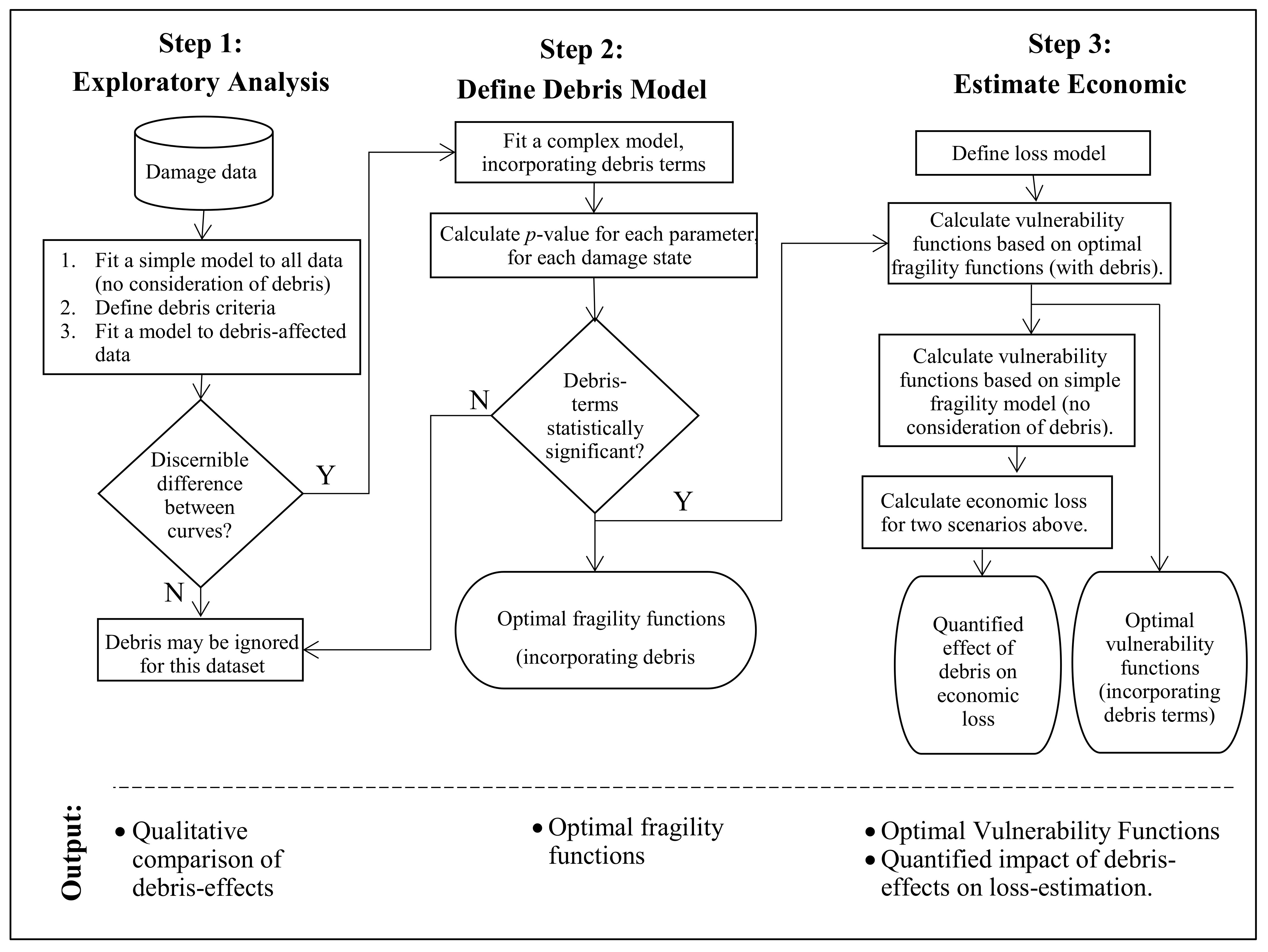
4.1. Step 1: Exploratory Analysis of Debris-Induced Bias (Case Study)
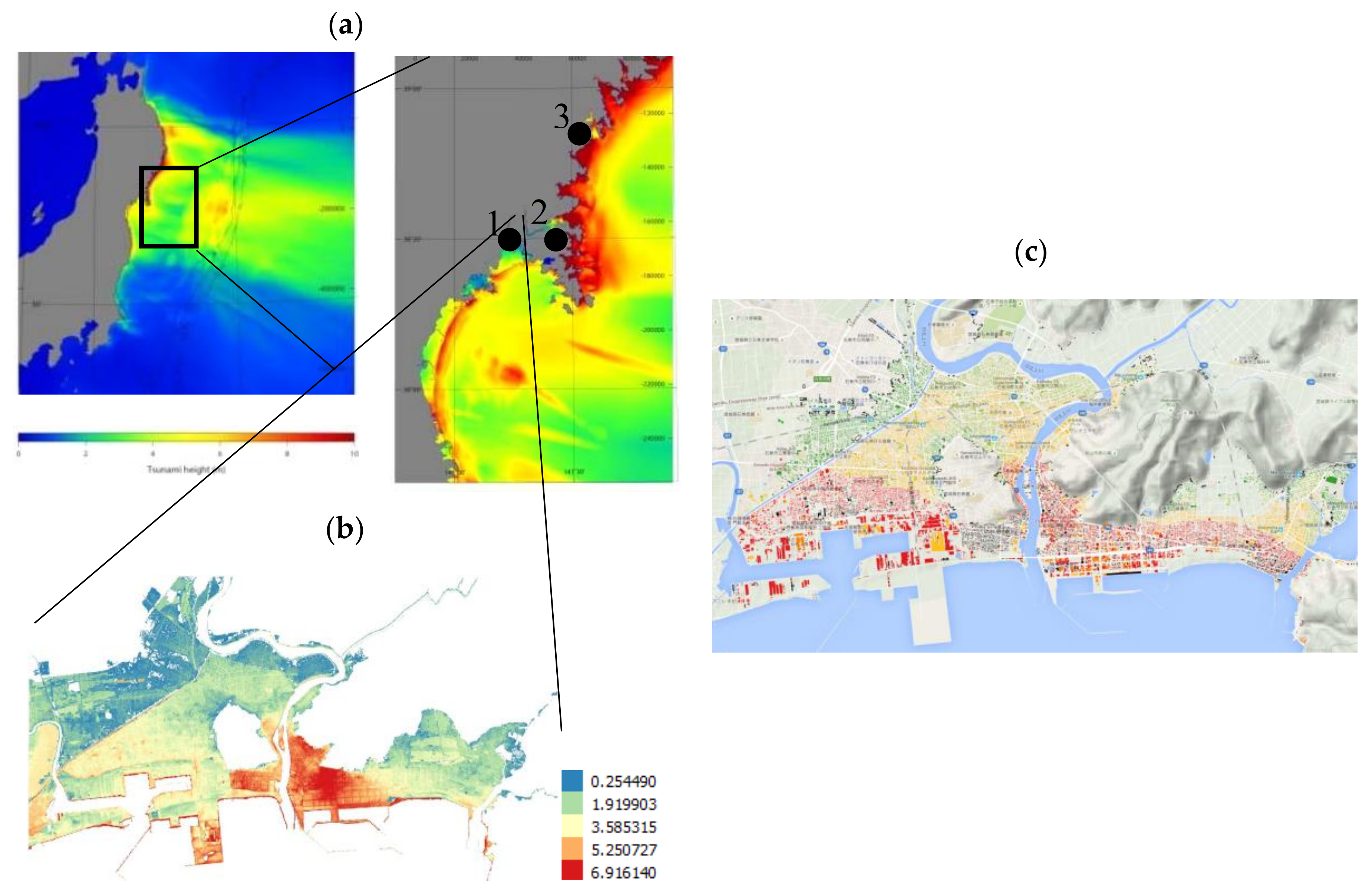
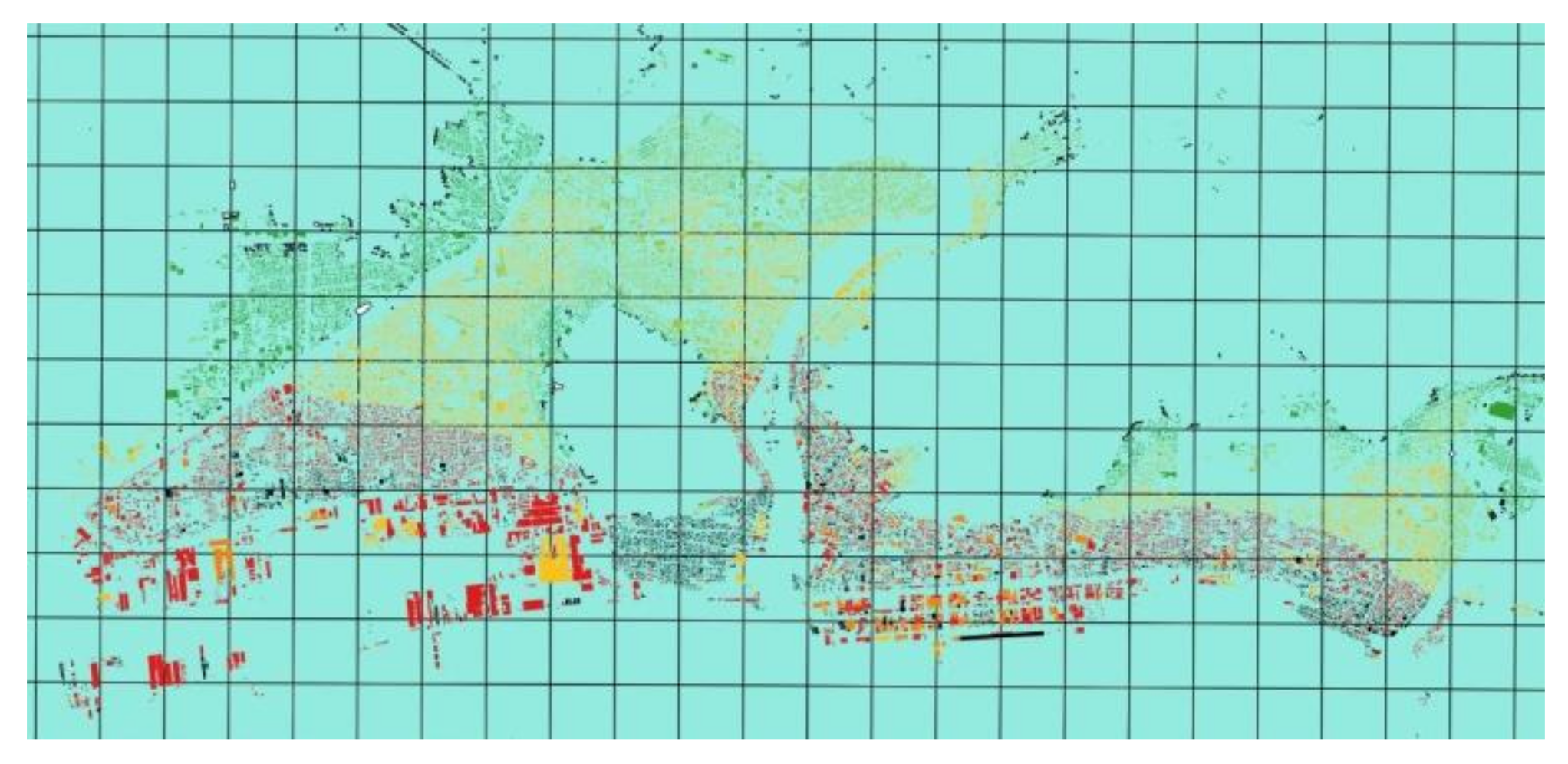
A regular grid of 500 m is applied to each case study location (
Figure 5). The total footprint area of all “washed away” (DS6) buildings is calculated for each grid square. If this area exceeds a threshold proportion of the total building footprint area for that grid all buildings of that grid square are designated as having been affected by debris. The levels of threshold proportions (i.e., washed away area/total area) are selected arbitrarily, and for the needs of this study three levels are tested: 20%, 35% and 50%.
Table 2 shows the number of buildings in the grid squares deemed to be affected by debris. As expected, the lowest collapse area threshold (of 20%) leads to the greatest number of buildings being removed from the dataset. Examining the damage states, inundation depths and forces experienced at building locations shows that buildings affected by debris generally fall into higher DS categories and at higher tsunami intensities.
Fragility functions are formed for all engineered buildings, and for those designated as affected or unaffected by debris, for the 20%, 35% and 50% collapse area thresholds. Reference [
8] demonstrates that the optimal TIMs for this dataset are inundation depth and a measure of force, and so both of these TIMs are adopted here. Partially-ordered cumulative link models with a probit link function (model (2)) are formed on the logarithms of the selected TIMs, as this model is shown by [
8] to fit this dataset well.
The fragility functions formed for all engineered buildings (i.e., the complete 4570-building dataset, ignoring debris) are considered as the base-case. It is seen that fragility functions for buildings with/without debris-impact deviate from the base-case, with the size of that deviation increasing with lower threshold values (i.e., the greatest deviations are seen for functions formed on data for the 20% collapse area threshold).
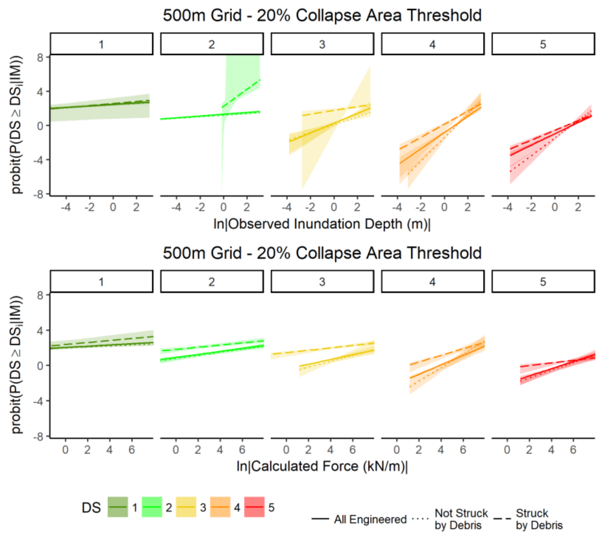
Figure 6 therefore compares fragility functions formed for all engineered buildings, and for those designated as affected or unaffected by debris, for the 20% collapse area threshold (visible trends are similar for the 50% and 35% thresholds). Note that
Figure 6 is plotted in link-space such that the x- and y-axes are transformed (indicated in the axis titles) so that the fragility functions appear as straight lines (Equation (2)), allowing trends to be more easily seen.
Intuitively, lower damage exceedance probabilities are expected in the absence of debris-related damage (i.e., a given flow depth may be deemed as more likely to cause damage if debris is also present in the flow). Therefore, taking fragility functions formed for all engineered buildings as the base-case (solid line,
Figure 6), then the expected trend in
Figure 6 is that damage exceedance probabilities should be higher for functions formed on debris-impacted buildings (dashed line,
Figure 6) and lower for functions formed on buildings not struck by debris (dotted line,
Figure 6). This expected trend is indeed shown in
Figure 6, with some exceptions. For depth, the exceptions lie at lower depths for DS3 and very high depths at DS4 and DS5, where the damage exceedance probabilities for buildings not struck by debris are greater than the base case. For force, the exceptions lie at high force levels for DS4 and very high force levels for DS5 where the damage exceedance probabilities for buildings not struck and struck by debris are greater and lower than the base case respectively. Consider that for the expectation to be upheld at all TIM values then the curves must be perfectly parallel, but the methodology used does not prescribe this, meaning that they will inevitably cross at some point. It may therefore be that these highlighted, counterintuitive instances are due to a lack of data at these TIM ranges to constrain the functions. This crossing of the curves can be prevented by including the debris term within the model (and omitting an interaction term, so that the curves remain parallel), as will be conducted in Step 2 below.
It can be seen in
Figure 6 that the confidence intervals at lower damage states are wider for buildings struck by debris, which reflects the fact that there are not many debris-affected buildings at these lower damage states. I.e., Buildings in the vicinity of other washed away buildings, DS6, are likely to have experienced higher damage states themselves. This is intuitive, as it would be expected that debris-affected buildings should experience greater damage. It can also be seen that confidence intervals are narrower for force (
Figure 6, bottom) compared to depth (
Figure 6, top), which might be considered to indicate reduced uncertainty when considering force as a TIM.
Therefore, the exploratory analysis presented in
Figure 6 demonstrates that the consideration of debris effects has a sizeable impact on the resulting fragility functions, and so this impact should be quantified in Step 2 of the methodology, below.
4.3. Step 3: Quantification of Impact on Financial Loss Estimation (Case Study)
Section 4.2 demonstrates that debris effects influence fragility function derivation. However, the question remains as to what impact this might have on the estimation of expected loss (E[L]) derived from those fragility functions. Equation (6) shows that accurate calculation of E[L] requires information on the value of the property and on the expected MDR for each damage state. The accurate definition of property value and expected MDR requires financial data which is beyond the scope of this paper. Hence, an approximate comparison of representative calculated losses is presented here to illustrate the impact that debris-effects can potentially have on loss forecasting.
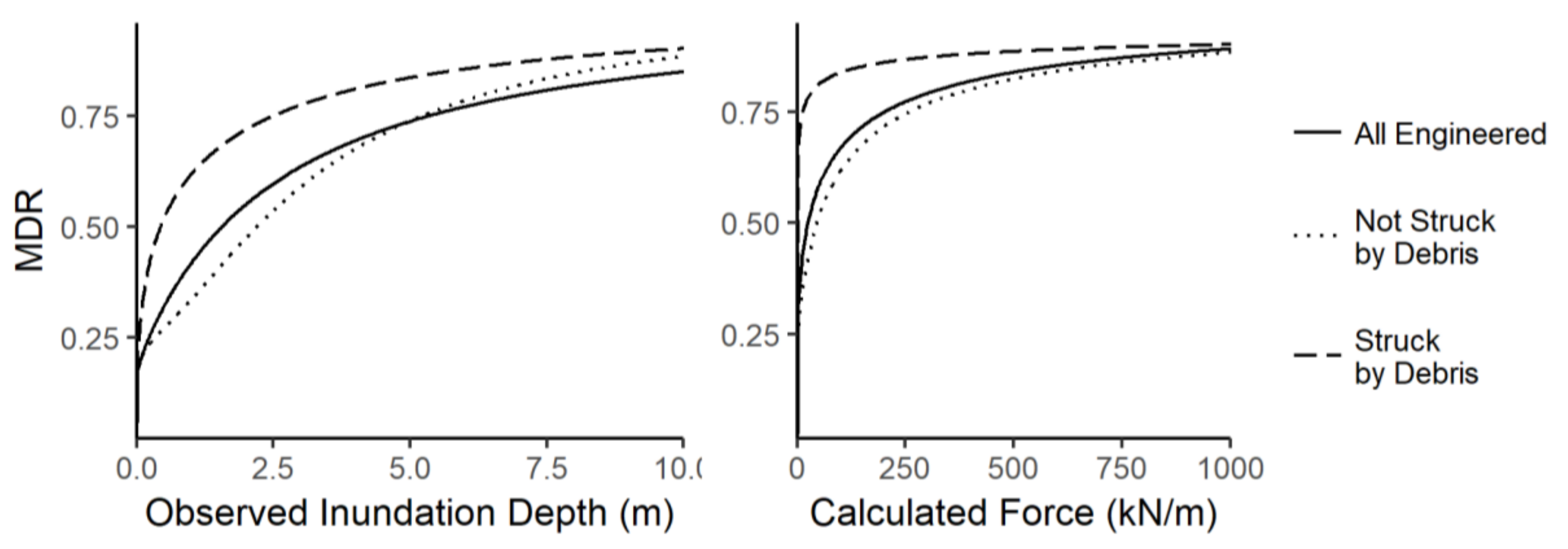
Preliminary vulnerability functions according to models (1) and (4) (considering only tsunami intensity, and incorporating debris, respectively) are shown in
Figure 7. As per [
22,
23,
24] and [
25], MDRs of 0, 5, 20, 40, 60, and 100% are assumed for DS0, DS1, DS2, DS3, DS4, and DS5, respectively. The buildings considered for the loss estimation are the same engineered structures (presented in
Section 2.1) used for the fragility derivation. The inundation scenario considered is the same 2011 Tsunami inundation presented in
Section 3.2. In the absence of more recent and site-specific financial data a mean unit construction cost of 1600
$/m
2 is assumed as per [
22,
24,
25]. The total construction cost for each building is then calculated by multiplying the unit construction cost by the footprint area and the number of stories. The total economic losses (the sums of expected loss for all the buildings in the dataset) are compared in
Table 5.
Figure 7 shows that, as expected, the MDR for buildings which are not struck by debris are lower than those struck by debris, and generally lower than that when ignoring the effect of debris (except at higher inundation depths, the reason for which should be investigated in future studies).
Table 5 shows that considering the effect of debris lowers the loss-estimate by between 1–1.5%, amounting to approximately 100
$M–150
$M in this particular scenario.
It is highlighted that the vulnerability functions cross at high values of inundation depth because of a lack of data with which to constrain the curves for this TIM range. This could be treated by removing the debris interaction term (β3 in Equation (3), so constraining the curves to be parallel.
Given a paucity of publicly available financial data, it is not possible to compare these results with observed losses during the 2011 Japan Tsunami, but this illustrative example serves to demonstrate that ignoring debris (or assuming that it is implicitly captured in the modelled inundation TIM), may lead to biases in loss estimation.


