Article

High Resolution Satellite Images for Instantaneous Shoreline Extraction Using New Enhancement Algorithms

by
Donatella Dominici
1,*,
Sara Zollini
1,
Maria Alicandro
1,
Francesca Della Torre
2,
Paolo Massimo Buscema
2,3 and
Valerio Baiocchi
4
1
DICEAA, Department of Civil, Environmental Engineering and Architecture, Via Gronchi 18, 67100 L’Aquila, Italy
2
Semeion Research Center of Sciences of Communication, Via Sersale 117, 00128 Rome, Italy
3
Department of Mathematical and Statistical Sciences, University of Colorado, Denver, CO 82017, USA
4
DICEA, Facoltà di Ingegneria, Sapienza Università di Roma, via Eudossiana, 18, 00184 Roma, Italy
*
Author to whom correspondence should be addressed.
Geosciences 2019, 9(3), 123; https://doi.org/10.3390/geosciences9030123
Submission received: 28 January 2019 / Revised: 20 February 2019 / Accepted: 28 February 2019 / Published: 11 March 2019

Abstract

:
Knowledge of a territory is an essential element in any future planning action and in appropriate territorial and environmental requalification action planning. The current large-scale availability of satellite data, thanks to very high resolution images, provides professional users in the environmental, urban planning, engineering, and territorial government sectors, in general, with large amounts of useful data with which to monitor the territory and cultural heritage. Italy is experiencing environmental emergencies, and coastal erosion is one of the greatest threats, not only to the Italian heritage and economy, but also to human life. The aim of this paper is to find a rapid way of identifying the instantaneous shoreline. This possibility could help government institutions such as regions, civil protection, etc., to analyze large areas of land quickly. The focus is on instantaneous shoreline extraction in Ortona (CH, Italy), without considering tides, using WorldView-2 satellite images (50-cm resolution in panchromatic and 2 m in multispectral). In particular, the main purpose of this paper is to compare commercial software and ACM filters to test their effectiveness.

1. Introduction

Italy is experiencing a number of environmental problems, including considerable coastline variations. The data available on coastline variation are of considerable concern: the extent of beach erosion exceeds the magnitude of sedimentation [1,2]. This represents a great threat, not only to the national heritage and economy, but also to human life. The coastal environment is the transition zone between the land and the sea. The shoreline is the strip of land that delimits a natural body of water. It differs from coastline, which is a strip of land of indefinite length and width that extends inland starting from the shoreline [3]. Why does the problem of studying and monitoring the shoreline arise? The coastal environment is a dynamic ecosystem, in which erosion phenomena are influenced by numerous factors including meteorological/climatic, geological, biological, and anthropic elements [4]. As is widely known, in the literature, there are different definitions of the shoreline, while generally, the surveying techniques acquire only the instantaneous shoreline. Shoreline is defined as the theoretical line of contact between land and water, something which is easy to establish, but very difficult to map because of its dynamic nature and the fact that water levels change continually [5]. In addition, geomatics techniques can detect the position of the land–sea interface at a given moment, which can be the same for the entire area under study, using some techniques, for example satellite acquisition [6,7]. With other geomatics techniques, the instant shoreline cannot even be acquired all at once, such as using GNSS receivers in RTK mode for which the line has to be measured in a time interval of up to several minutes. This factor makes ground data generally not directly comparable with data from aircraft or satellites. Here, however, the interest is to evaluate the different techniques for extracting the instantaneous shoreline, as it is visible in one or more satellite images. Shoreline erosion can damage buildings and infrastructure (roads, railways, etc.) and lead to risk of flooding in coastal areas. Important ecosystems and areas of great biodiversity are risking destruction or severe impoverishment. Italy’s coastal development is approximately 8300 km in length, and the natural coastline is about 7500 km long. More than 9% of the coastline is now artificial and bordered by work close to the shoreline (3.7%), ports (3%), and structures partially superimposed onto the coast (2.4%). About 3250 km of this is sandy coastlines [1,2]. There are many cases in which coastline erosion is putting the safety of homes, roads, and railways in danger, especially during storms. Coastal areas are the most densely occupied by urban settlements and economic and productive activities. According to updated ISPRAdata [1,2], from 1950–1999, 46% of low-lying coastal areas underwent changes exceeding 25 m, and in particular, there are more stretches of coastline subject to erosion than sedimented ones. Analysis of the 2000–2007 changes has confirmed this trend: 37% of the coastline underwent variations of over 10 m, and quantities of coastline subject to erosion (897 km) were still higher than those in progradation (Table 1).

State-of-the-Art of Shoreline Detection

There is no single method for modeling the shoreline, although over the last ten years, great progress has been made in mapping technology, ranging from the development of new and increasingly-precise measurement techniques such as GNSS (Global Navigation Satellite System) to high and very high resolution satellite images and the development of particularly efficient devices for coastal topography assessment. The most common methods currently used for the identification of the shoreline include:
  • Traditional topographical surveys (leveling, surveys with total stations) and GPS [8,9,10]: These allow high precision measurements in individual points, without any possibility to repeat the survey;
  • Video systems [8,9]: The technique is used mainly with a network of fixed terrestrial cameras (e.g., ARGUS [11]) and Siren) from a few units up to tens, installed at prominent points in the landscape or on specially-positioned supports. They acquire at intervals of up to 10 hz, encompassing 180° views and allowing total coverage of about 4–6 km of beach. The acquired images are oblique and require orthorectification operations, as well as georeferencing with algorithms derived from classical photogrammetry;
  • Aerophotogrammetric/UAV survey [12,13,14,15,16,17,18,19,20]: This does not provide a detailed relief, but represents the entire study area at the time of acquisition. Achievable precisions are at the centimeter-subcentimeter level, but the costs are high. “Ad hoc” flights must be planned, and above all, it is significantly influenced by weather conditions (sunny and minimal wind conditions are needed); this leads to limitations on flight seasons;
  • Satellite remote sensing [21,22]: This refers to the latest-generation remote sensing satellites, which are becoming more effective as compared to those available previously. Traditionally, medium resolution satellites (e.g., Landsat and Sentinel-2) have been used advantageously for coastline studies that did not require very high accuracy. Satellites with high and very high resolution are required because they are particularly advantageous compared to traditional photogrammetric aerial acquisitions. High spatial resolution remote sensing satellites allow data to be acquired and processed more quickly, with comparable precision, while offering a very high level of detail. Furthermore, the fundamental ability to capture the scene in several spectral bands allows more information to be extracted than is extractable from images covering only the visible part of the electromagnetic spectrum and thus allows thematic maps of the territory to be created through multispectral classification. Another advantage, which makes this technique more attractive than the others, is that satellite revisit times are very short (a few days), which allows the area to be studied on images taken at different times.
From the literature, it is clear that the use of satellite images is the most diffused for the coastal environment by now, and this paper will deal with the study of innovative filters for the extraction of the shoreline. This work is a first step for a comparison between ACM filters (never used in the engineering fields) and filters well known in the world of the software used.

2. Case Study

The following experimentation concerns the shoreline in Ortona (CH, Italy) using WorldView-2 satellites. Common filters were initially used. Then, ACM filters were tested and compared with previous ones. The images were visually analyzed in order to find rapid ways to extract the instantaneous shoreline.

2.1. WorldView-2

WorldView-2 satellites acquire eight-band multispectral images with a resolution of 2 m to provide the best natural representation of the Earth from space, and panchromatic images with a resolution of 50 cm [23]. In particular, WorldView-2 is the first commercial high resolution satellite capable of acquiring, in addition to the four typical blue, green, red and near-infrared bands, four additional multispectral bands, previously unavailable on a very high resolution satellite: coastal, yellow, red edge, and Near Infrared 2 bands [23]. The coastal band is designed to study the shoreline, because of its ability to penetrate under the water’s surface. WorldView-2 operates at an altitude of 770 km, and its advanced onboard system is capable of capturing images above the Earth [23]. These images provide unprecedented detail, enabling very accurate detection.

2.2. Data Pre-Processing

The “raw” images of Ortona’s coastline, taken by the WorldView-2 satellite (Figure 1) by DigitalGlobe on 29 June 2010, contain geometric and radiometric distortions, so specific software based on rigorous algorithms or based on rational polynomials must be used to correct them. The panchromatic and multispectral images are georeferenced to the WGS84 reference system (WGS84/UTM Zone 33 N, EPSG: 32633).
The image correction steps are [21,24]:
  • orthorectification;
  • georeferencing;
  • resampling;
  • pansharpening.
For the Ortona images, 23 GCPs (Ground Control Points) were acquired during a previous research [21] by means of double-frequency GNSS receivers and processed in post-processing mode compared to the network of permanent stations of the Abruzzo region [6]. Eight of these were used as CPs (Check Points), to evaluate the accuracy of the measurements. To take into account land elevations, the basis for the relief displacements due to terrain elevations, DEM in software library was used. To correct geometric distortion of WorldView-2 satellite images, Rational Polynomial Coefficients (RPCs) were used. After that, we proceeded with a resampling, using the nearest neighbor technique. Then, the “HCS (Hyperspherical Color Space) Resolution Merge” technique was adopted [25] to perform pansharpening.
After these steps were complete, the images were ready to be processed using the so-called “enhancement techniques”.

2.3. Data Processing with Common Filters

A series of filters (enhancement technique) [26] was tested on the image (in this experimentation, ERDAS IMAGINE 2015 software was used) to find the best ones that showed a clear and defined shoreline.

2.3.1. Decorrelation Stretch

The first step is PCA (Principal Component Analysis), which is used in statistics for the simplification of source data. It is often used as a data compression method: it allows redundant data to be compressed into fewer bands using linear transformation. Four bands were chosen (coastal, red, green, and blue bands) [24]. Then, the decorrelation stretch filter was applied. This allows the whole range of DN (Digital Numbers) varying from 0–255 to be used and, therefore, a greater amount of information to be extrapolated. The decorrelation stretch is a sort of “stretching” that is applied only to the chosen four bands (which are called “main components”) and not to the original image. The potential of this technique is exploited to highlight the elements that are almost invisible to the naked eye, to improve and facilitate visualization. The resulting image enabled clear shoreline distinction due to the radiometric response of the elements on the Earth’s surface (Figure 2).
In Figure 2, the darker color of the water indicates the presence of shallow waters, which correspond to artificial barriers (used to mitigate the erosive effect of the sea). The difference between wet and dry sand is revealed in the change of color from dark red to light red, respectively.

2.3.2. Normalized Difference Vegetation Index

The NDVIs [27] are mainly used for forests or related to agriculture applications [28,29,30], but they also give excellent results in shoreline definition. As is well known, the main objective of this index is to analyze the differences between the characteristic components of the vegetation’s spectral signature. This denominator assumes the role of normalization factor, while the relevant characteristic of the index is the numerator. NDVI combines the red and the near-infrared (Equation (1)) pixel by pixel:
N D V I = N I R R E D N I R + R E D
According to this definition, NDVI ranges mathematically between −1 and +1, but, in practice, between −0.4 (water bodies) and +0.7 (very dense and broad-leaved vegetation). In general, still water has low reflectance. In addition, NDVI is able to compress the size of the data by a factor of two because it replaces two spectral bands with a single band. The result computed for the shoreline is shown in Figure 3.
The shoreline between water and beach is visually well defined: the contrast between them is much accentuated by the abrupt transition between black and white, respectively.

2.3.3. WorldView Water Index

The WorldView Water Index (WV-WI) proved to be the most powerful algorithm. Above all, it is specific to images taken by WorldView satellites and, therefore, suitable for this case study. It is good for detecting water or shadows [24]. Traditionally, the blue band is normalized with the NIR2 band, because the radiometric answer is clearly visible. The WorldView Water Index considers coastal and NIR2 bands [24] (Equation (2)) because the difference between these bands, in terms of wavelengths, is greater (coastal band 400–450 nm, blue band 450–510 nm, NIR2 band 860–900 nm [27,31]), so it provides an even more discreet threshold to identify water rather than land or vegetation areas:
W V W I = C B N I R 2 C B + N I R 2
The results of applying it to the WorldView-2 Images are shown in Figure 4:
Water has a much higher value on the coastal blue band than on the NIR2 band: this is why it is white in color. The contrast between the water and the ground is very high. The differences between deeper and less deep water and even between dry and wet sand are not evident, but this algorithm is definitely the best of those tested from the point of view of shoreline definition because it shows a clear contrast between water and land.

2.3.4. Unsupervised and Supervised Classification

“Classification” refers to the grouping of pixels and similar values into groups (called “clusters”) that identify a specific category within the data [4]. Pixels are divided into categories based on their spectral properties. The most delicate problem is defining the type and number of classes. As is well known, there are two types of classifications: unsupervised and supervised. K-means and ISODATA algorithms were used for the unsupervised classification [24], taking 30 clusters into account. In the supervised classification, 12 clusters were identified, and the maximum likelihood parametric method was used [4].
The shoreline derived from both methods is well defined (Figure 5), but the main information that can be extrapolated in the results of unsupervised classification is the difference in depth in the various areas of water (from deep to less deep water, color degrades from blue/grey, pink, blue, orange, to light blue at the shore). The same can be said for the difference between dry and wet sand where the drier sand is green, while wet sand varies from light blue to red. Comparing the results of supervised classification into 12 classes with unsupervised classification into 30 classes, the supervised classification reveals less information about sea depth.

2.4. Data Processing with the ACM System

In this section, some experimental algorithms are tested on WorldView-2 images to determine their effectiveness for the case study. These algorithms have been developing by Professor Paolo Massimo Buscema, mathematician, Director of the Semeion Research Centre of Science of Communication of Rome and Full Professor Adjoint at the University of Colorado (USA).
This patent concerns Active Connections Matrix systems (ACM), according to which each image is considered as an active matrix (network) of connected elements (pixels) that develops over time. The main idea upon which this theory is based states that each digital image stores the maximum amount of information within the pixel values and their relationships. Furthermore, it is possible to obtain important information by analyzing the reciprocal positions occupied by pixels. For a complete presentation of ACM algorithms, see [32,33].
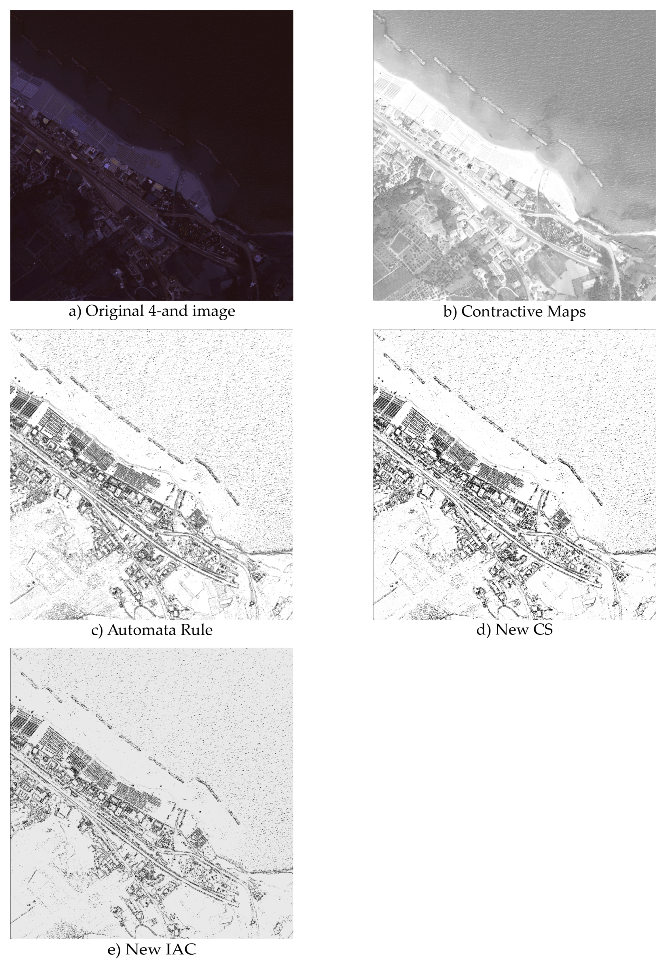
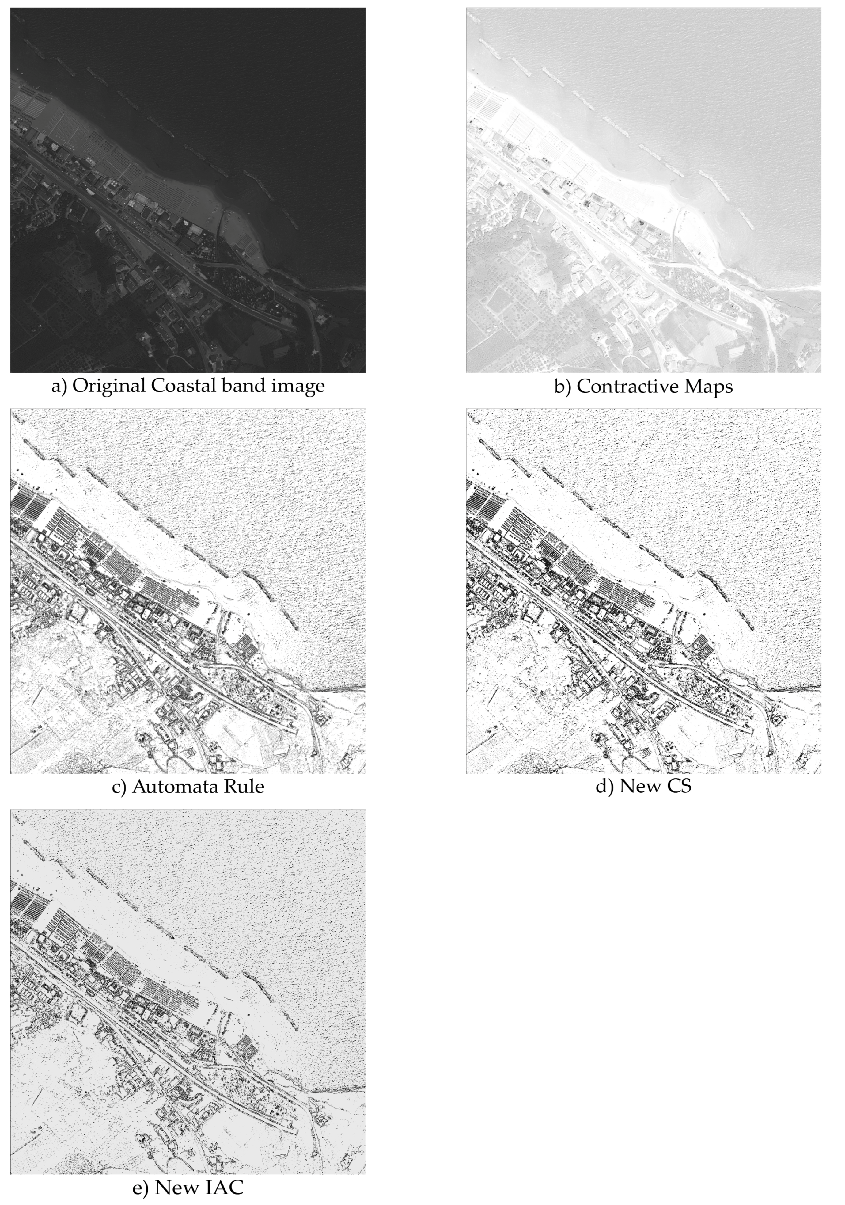
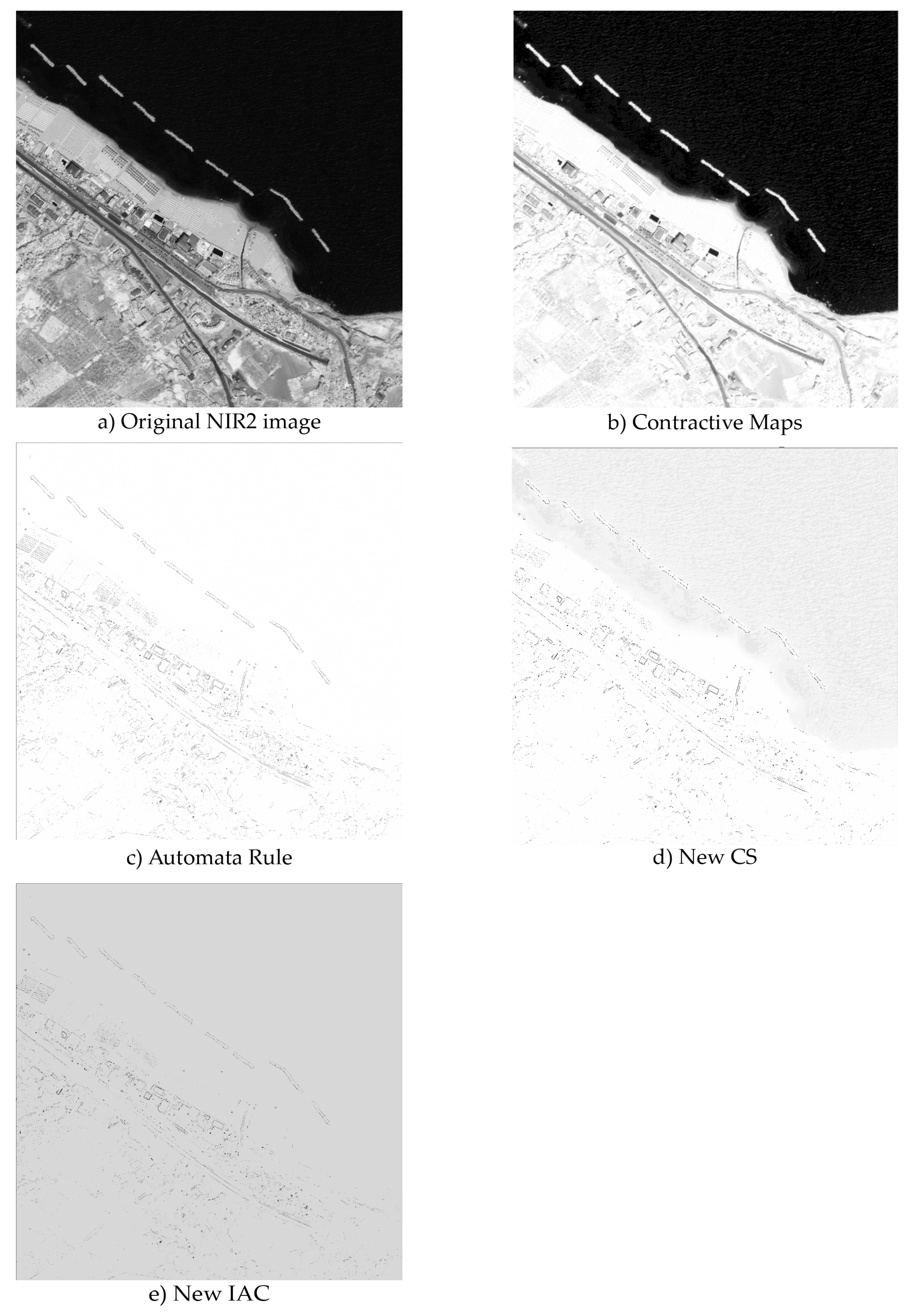
Any digital image is a matrix made of as many rows as the pixels that determine the width and as many columns as the pixel related to the height. Each pixel is identified by its coordinates i 1 , , R , j 1 , , C and its brightness L 2 M (e.g., in the case of 256 shades of grey, M = 8 ). For each pixel u i j , a set containing all the surrounding pixels I ( u i j ) named the neighborhood can be defined. In the ACM systems, all the pixel u x y I ( u i j ) are linked to the central pixel u i j by means of the w ( i j ) , ( x y ) connections. Figure 6 shows what is meant by neighborhood and the meaning of w connections in the case of r a d i u s = 1 . Obviously, it is possible to use a larger radius by extending the number of pixels to be considered as the neighborhood. The systems are classified into three orders of complexity, according to the type of evolution over time. In the first order of complexity, the values of connections are initialized once, at the beginning, and then remain fixed while pixel values u i j [ n ] evolve over time until convergence, starting from the u i j [ 0 ] value, directly derived from the image. The situation is specular in the case of second order, where the pixels values are fixed and equal to u i j [ 0 ] , while the connections values w ( i j ) , ( x y ) [ n ] are updated at each iteration, after initializing them to values w ( i j ) , ( x y ) [ 0 ] 0 . Finally, the third order of complexity includes models in which both the pixels and the connections change over time. The following algorithms were used in this project: Automata Rule (AR), New Interactive Activation and Competition (New IAC), New Constraint Satisfaction Networks (New CS), Contractive Map (CM), and J-Net Dynamic. The authors decided to describe the algorithms in detail in Appendix A to avoid boring readers of the paper.

2.5. Analysis of Results

For the case study, software “ACM Batch” was used [34]. To test possible similarities or differences, the algorithms were tested on:
  • a four-band image (coastal, red, green, and blue);
  • an image containing only the coastal blue band (which is specific for coastal studies);
  • an image with the coastal blue band plus NIR2;
  • an image with only the NIR2 band.
These choices were carried out because these bands best respond to shoreline detection. In this paper, for the sake of brevity, the results are shown in Appendix B. Here, only the results obtained by applying the contractive maps on the NIR2 image are shown in Figure 7a, because it had similarities with two of the common filters: NDVI and WVWI (Figure 7b,c).
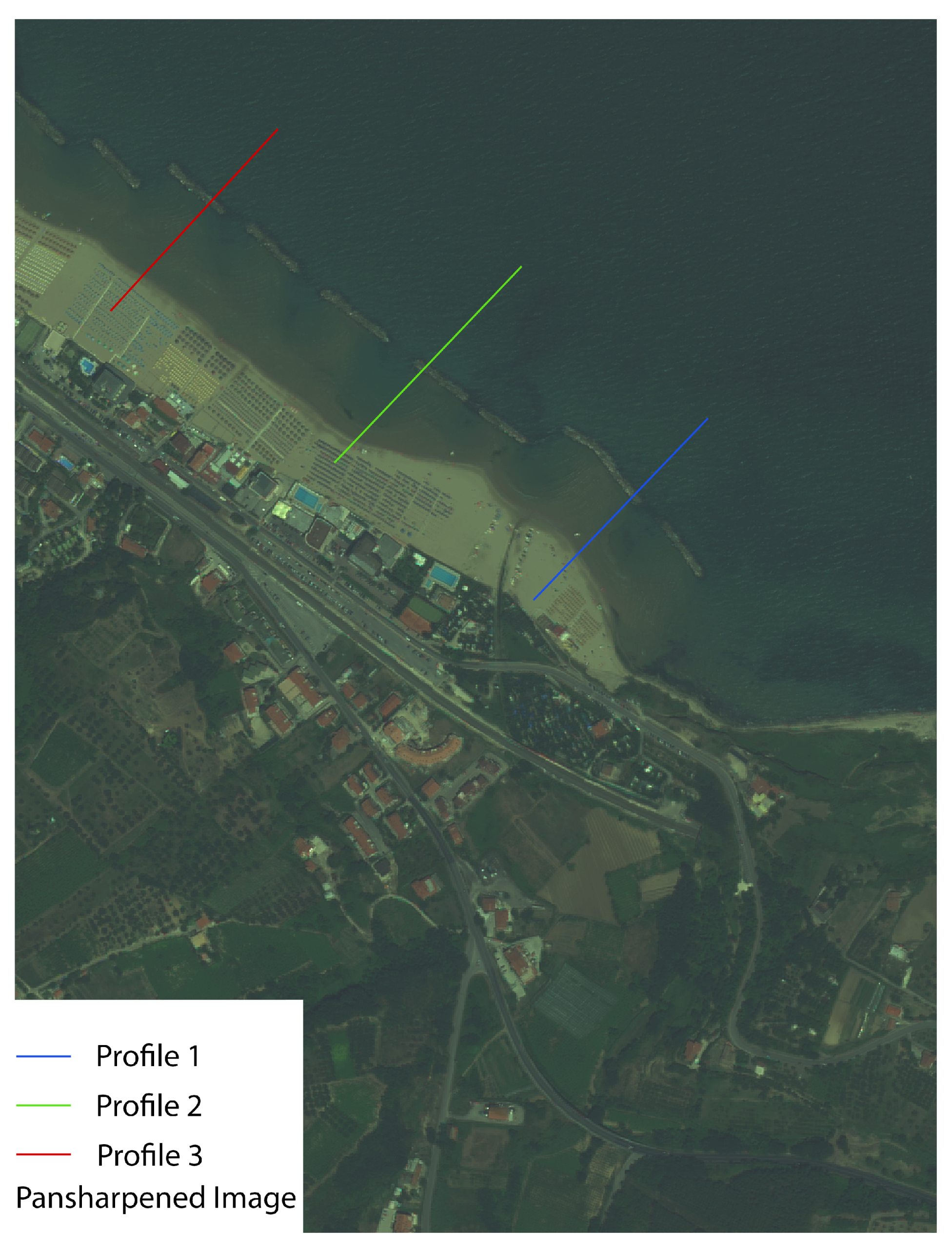
In every image, the high reflectance between land and water shows a defined shoreline, which is metrically detected taking three profiles (diagrams of the pixel values as a function of a distance) over three sample distances. As a reference, a pansharpened image is considered (Figure 8). In this image, every color corresponds to a profile, and in particular, Profile 1 is blue, Profile 2 green, and Profile 3 red. These colors will be the same as the profiles plotted in Figure 9.
The letter “A” refers to the shoreline extracted from the pansharpened image, used as a reference. It is also worth noting the peaks at the rocks (Lines B and C) because they show similar trends in almost all the graphics. Line D in Figure 9 refers to the shorelines extracted from, respectively, NDVI, WVWI, and CM over NIR2 images. Line D was determined in correspondence with the maximum slope on the jump for the CM over the NIR2 image and in correspondence with the middle point of the jump for the NDVI and WVWI. The differences between the reference image (pansharpened, Line A) and the other filter (Line D) was studied. It is shown in Table 2. For Profile Number 2 on the NDVI image (Figure 9b) and Profile 3 on the WVWI image (Figure 9f), there was not a clear jump, which emphasizes the shoreline, as in the other cases. For this reason, Line D on these two graphs is not drawn.
As shown in the table, the differences were the same for Profile 1, but were closer to the value taken from the pansharpened image in the case of Profiles 2 and 3 for the CM filter.
A similar trend can be seen in the graphs. Peaks and hollows, which correspond to the passage from the mainland to the sea (and vice versa), are displayed at the same distance in all the graphs. In other words, in Profile 1, the first peak/hollow can be seen around 70 m and the second one around 150 m. This behavior is the same in all three for Profile 1 (Figure 9a,d,g). The same can be said for Profiles 2 (Figure 9b,e,h) and 3 (Figure 9c,f,i). This means that the algorithms worked in a very similar way. The original elaborations are shown in Appendix B.

3. Discussion of Results and Conclusions

In the present work, the potential of the ACM models for the automatic identification of the coastline from very high resolution multispectral satellite images has been tested. The interest for the definition of a certain and robust procedure in this regard derives from the increase in the phenomenon of coastal erosion that affects low coasts, as well as the Italian ones. The ACM models already successfully applied in other (mainly health) applications have been adapted and tested here for the first time on satellite images.
To verify the accuracy and robustness of this approach, the results of the experiments on a sample area were compared with those obtained on the same area using all the algorithms and filters most commonly used for these same applications [35].
By combining the various types of images with the various models, it was possible to obtain a wide range of tests in order to validate the model exhaustively on the specific test site. For space reasons, the complete results of all the tests have been reported in the Appendix B. From the above-mentioned experiments, we can give some general considerations on the ACM algorithms:
  • their ability to define the contours of real images was excellent;
  • their adaptation to satellite imagery made them a powerful tool for digital image processing, and they can be used for automatic territory analysis;
  • they were capable of distinguishing noise and salient forms within the image.
More in detail, we can say that by comparing the profiles obtained automatically by the various algorithms, the ACM models always showed an accuracy greater than or equal to that of the most common methodologies. Moreover, the measured deviation from what can be observed on the screen was always the result of the order of the pixel and often subpixel, making the method even more accurate than the much more expensive manual acquisition.
This is potentially very useful for future change detection between two images taken in different time periods, generating a concrete possibility that an appropriate intervention plan can be developed, indispensable if government institutions, such as civil protection agencies, need to carry out rapid monitoring.

Author Contributions

The authors contributed equally to this work.

Funding

This research received no external funding.

Conflicts of Interest

The authors declare no conflict of interest.

Abbreviations

The following abbreviations are used in this manuscript:
ACMActive Connections Matrix
GPSGlobal Positioning System
WGS84World Geodetic System 1984
GCPGround Control Point
CPCheck Point
DNDigital Number
HCSHyperspherical Color Space
PCAPrincipal Component Analysis
NDVINormalized Difference Vegetation Index
WVWIWorldView Water Index
ARAutomata Rule
New IACNew Interactive Activation and Competition
New CSNew Constraints Satisfaction Network
CMContractive Maps
Anti-CMAnti-Contractive Maps

Appendix A.

In the following, the most useful algorithms for this case study will be illustrated.

Appendix A.1. Automata Rule

The Automata Rule (AR) [32] serves to initialize the values of the connections in the ACM with fixed connections (first order of complexity). This algorithm defines the connections between each pixel-unit as a non-linear transformation of their different brightnesses:
w ( i j ) , ( x , y ) [ 0 ] = t a n h ( R ( i j ) , ( x y ) )
where:
R ( i j ) , ( x y ) = c 1 ε ( 2 · R ( i j ) , ( x y ) ε 1 )
R ( i j ) , ( x y ) = e ( σ · u i j σ · u x y ) 2 , 0 σ 2 N
ε = e σ 2
The parameter σ serves to modulate the connection strength. The values obtained with Equation (A1) are close to one the more the brightness values are similar to each other. In this case, R ( i j ) , ( x y ) 1 , so that R ( i j ) , ( x y ) c . The c value is a scale factor useful to make the calculations easier since it moves the R ( i j ) , ( x y ) value into the [ c , c ] interval (e.g., c = 5 ). As for the weights’ initialization, the automata rule can also be used as a filter on the initial image. A new image will be created where each pixel value u i j A R is the average of all the weights connecting u i j with each pixel of its neighborhood (see Equation (A5)):
u i j A R = 1 | I u i j | · u x , y u i j w ( i , j ) , ( x y )
The resulting image will highlight the edges of the pictures in the image. In fact, the more pixels are similar, the more the connection values will look like one (white), so the mean rate will be high. If the pixels have different values, the weights will be closer to −1 (black), as will the average.

Appendix A.2. New IAC

As with all the ACM algorithms, New Interactive Activation and Competition [32] (New IAC) considers each pixel as an agent connected to the others in its neighborhood. The connections linking u i j to all the u x y I u i j are initialized by means of the automata rule, then they remain fixed until the end of the process; therefore, New IAC belongs to the first order family. Each u i j receives excitations and inhibitions from the surroundings and changes its state accordingly at each iteration. Equations (A6) and (A7) allow the computation of the excitation and inhibition values released by the neighborhood of the pixel u i j at the iteration n. Equation (A8) determines the input arriving at it as a weighed sum of those quantities. The final value of the activation of the pixel u i j is then computed by means of Equation (A9):
E i j n = u x y I u i j u x y [ n ] · w ( i j ) , ( x y ) · χ { w ( i j ) , ( x y ) > 0 } ( w ( i j ) , ( x y ) )
I n i j [ n ] = u x y I u i j u x y [ n ] · w ( i j ) , ( x y ) · χ { w ( i j ) , ( x y ) < 0 } ( w ( i j ) , ( x y ) )
where χ A is the indicator function, i.e., χ A ( x ) = 1 if x A , otherwise χ A ( x ) = 0 ;
N e t i j [ n ] = α · E i j [ n ] + β · I n i j [ n ]
A c t i j [ n ] = t a n h ( N e t i j [ n ] )
The α and β parameters modulate the influence of inhibitory and excitatory stimuli coming from the neighborhood. A frequent choice is to place α = β = σ 2 M . The value of each pixel changes over time, and step by step, new values are computed based on the value that it had in the previous iteration and a quantity, named Δ i j [ n ] , which takes into account the A c t i j [ n ] value, i.e., u i j [ n + 1 ] = f ( u i j [ n ] , Δ i j [ n ] ) . Equation (A10) shows how this function works:
u i j [ n + 1 ] = u i j [ n ] + t a n h ( Δ i j [ n ] )
Δ i j [ n ] = [ ( M u i j [ n ] ) · A c t i j [ n ] d · ( u i j [ n ] r ) ] · χ { A c t i j [ n ] 0 } ( A c t i j [ n ] ) + [ ( u i j [ n ] m ) · A c t i j [ n ] d · ( u i j [ n ] r ) ] · χ { A c t i j [ n ] < 0 } ( A c t i j [ n ] )
where M and m are the maximum and minimum value that the pixels’ value can take on and d and r are two learning coefficients related to the decay and the rest of the updating units, usually M = 1 , m = 0 , while d = r = 0 . 1 . It is possible to say that New IAC allows the pixels to coordinate themselves by exploiting the connections determined by AR. The areas where the pixel brightness is similar are moved toward white, while when where there are sudden changes in luminance, the relevant pixels are led to dark.

Appendix A.3. New CS

New Constraints Satisfaction Network [32] (New CS) is an ACM system with fixed connections based on the constraint satisfaction network model [1]. The main idea behind New CS is to consider each pixel-agent of the matrix as a “hypothesis”, which may be true or false in a fuzzy way, in relation to the brightness of the pixel itself. New CS tries to make every hypothesis of the matrix “true” by maximizing the brightness of each pixel-agent, having as a constraint the value of fixed connections previously calculated with AR (Equations (A1)–(A4)). The maximization problem to solve is then:
M a x 1 2 · i { 1 , . . . , R } , j { 1 , . . . , C } u x y I i j u i j · u x y · w ( i j ) , ( x y )
s . t .
u i j [ 0 , 1 ] i { 1 , . . . , R } a n d j { 1 , . . . , C }
w ( i j ) , ( x y ) = t a n h ( R ( i j ) , ( x y ) ) i , x { 1 , . . . , R } a n d j , y { 1 , . . . , C }
To achieve the maximization requested in Equation (A12), the units’ values interact and evolve according to Equations (A13)–(A15):
N e t i j [ n ] = ( x y ) s . t . u x y I i j u i j [ n ] · w ( i j ) , ( x y )
Δ i j [ n ] = N e t i j [ n ] · ( 1 u i j [ n ] ) · α · χ { N e t i j [ n ] 0 } ( N e t i j [ n ] ) + N e t i j [ n ] · u i j [ n ] · α · χ { N e t i j [ n ] < 0 } ( N e t i j [ n ] )
u i j [ n + 1 ] = u i j [ n ] + Δ i j [ n ]
Thus, Δ i j [ n ] pushes the unit’s value towards higher or lower values according to the values of its neighborhood, weighted by the values of connections. The α value is a parameter for adjusting the magnitude of corrections, generally α = 1 . 0 .

Appendix A.4. Contractive Maps

Contractive Maps (CM) [32] belongs to the first order of complexity family. The initial values u i j [ 0 ] remain unchanged over time and act as a constant impulse of the system. On the contrary, connections evolve over time, leading to the creation of new images. Equations (A16)–(A18) show the w ( i j ) , ( x y ) [ n ] updating process. To make it more easily legible, all the occurrences of u i j [ 0 ] have been replaced by u i j ; furthermore, we use the parameter C = | I i j | :
N e t i j [ n ] = u x y · ( 1 w ( i j ) , ( x y ) [ n ] C )
A n t i N e t i j [ n ] = ( u x y ) 2 · w ( i j ) , ( x y ) [ n ] · ( 1 w ( i j ) , ( x y ) [ n ] C )
Δ w ( i j ) , ( x y ) [ n + 1 ] = N e t i j [ n ] · A n t i N e t i j [ n ]
At each iteration, a new image is drawn, i.e., new values P i j [ n ] for pixels must be computed. There exist different ways to do that, and Table A1 shows some of them.
Table A1. Some of the rules available to create new images.
NameEquation
Mean P i j [ n ] = 1 C · ( x y ) s . t . u x y I i j w ( i j ) , ( x y ) [ n ]
Variance P i j [ n ] = 1 C · ( x y ) s . t . u x y I i j 1 C · ( x y ) s . t . u x y I i j w ( i j ) , ( x y ) [ n ] w ( i j ) , ( x y ) [ n ] 2
Maximum P i j [ n ] = max ( x y ) s . t . u x y I i j w ( i j ) , ( x y ) [ n ]
Minimum P i j [ n ] = min ( x y ) s . t . u x y I i j w ( i j ) , ( x y ) [ n ]
At each iteration, the values of pixels of the image at the previous step are replaced by those computed by means of one of the methods of Table A1. Then, the values of connections are updated considering the original value of pixels. The process ends when the dynamic system reaches its attractor and Δ w ( i j ) , ( x y ) [ n ] 0 .

Appendix B.

Appendix ACM Elaboration
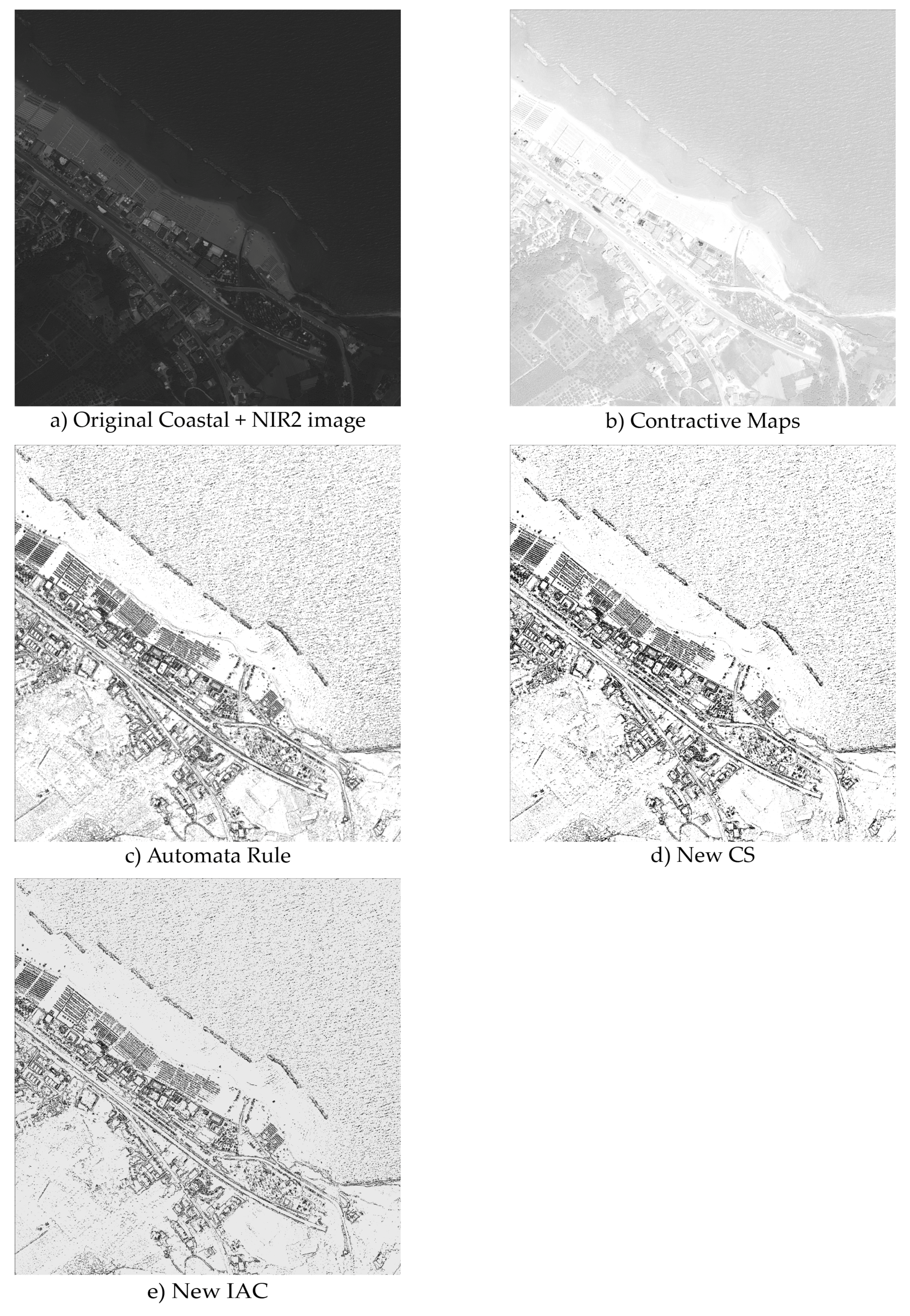
Figure A1. Four-band image elaborated by ACM filters.
Geosciences 09 00123 g0a1
Figure A2. Coastal image elaborated by ACM filters.
Geosciences 09 00123 g0a2
Figure A3. Coastal plus NIR2 band image elaborated by ACM filters.
Geosciences 09 00123 g0a3
Figure A4. NIR2 band image elaborated by ACM filters.
Geosciences 09 00123 g0a4

References

  1. Istituto Superiore per la Protezione e Ricerca Ambientale (ISPRA). Mare e Ambiente Costiero. 2011. Available online: http://www.isprambiente.gov.it/it/pubblicazioni/stato-dellambiente/ tematiche-in-primo-piano-annuario-dei-dati-ambientali-2011 (accessed on 17 October 2016).
  2. Istituto Superiore per la Protezione e Ricerca Ambientale (ISPRA). Mare e Ambiente Costiero. 2014–2015. Available online: http://www.isprambiente.gov.it/it/pubblicazioni/stato-dellambiente/ tematiche-in-primo-piano-annuario-dei-dati-ambientali-2014-2015 (accessed on 17 October 2016).
  3. Boak, E.H.; Turner, I.L. Shoreline definition and detection: A review. J. Coast. Res. 2005, 21, 688–703. [Google Scholar] [CrossRef]
  4. Lasalandra, M.G. Metodologia per la Mappatura Delle Spiagge e Della Dinamica Litoranea Mediante la Classificazione di Immagini Digitali, ISPRA, 2009. Available online: http://www.isprambiente.gov.it/contentfiles/00004400/4488-lasalandra.zip/atdownload/file (accessed on 23 January 2017).
  5. Aguilar, F.J.; Fernández, I.; Pérez, J.L.; López, A.; Aguilar, M.A.; Mozas, A.; Cardenal, J. Preliminary results on high accuracy estimation of shoreline change rate based on coastal elevation models. Int. Arch. Photogramm. Remote Sens. Spat. Inf. Sci. 2010, 33, 986–991. [Google Scholar]
  6. Baiocchi, V.; Dominici, D.; Ialongo, R.; Milone, M.V.; Mormile, M. DSMs Extraction Methodologies from EROS-B “Pseudo-Stereopairs”, PRISM Stereopairs in Coastal and Post-seismic Areas. In Computational Science and Its Applications—ICCSA 2013. ILecture Notes in Computer Science; Springer: Berlin/Heidelberg, Germany, 2013. [Google Scholar]
  7. Palazzo, F.; Latini, D.; Baiocchi, V.; Del Frate, F.; Giannone, F.; Dominici, D.; Remondiere, S. An application of COSMO-SkyMed to coastal erosion studies. Eur. J. Remote Sens. 2012, 45, 361–370. [Google Scholar] [CrossRef]
  8. Carli, S.; Cipriani, L.E.; Bresci, D.; Danese, C.; Iannotta, P.; Pranzini, E.; Wetzel, L. 6. Tecniche di Monitoraggio Dell’evoluzione Delle Spiagge. In REGIONE TOSCANA. Il Piano Regionale di Gestione Integrata Della Costa ai fini del Riassetto Idrogeologico. Erosione Costiera; EDIFIR: Firenze, Italy, 2004; pp. 125–192. [Google Scholar]
  9. Harley, M.D.; Turner, I.L.; Short, A.D.; Ranasinghe, R. Assessment and integration of conventional, RTK-GPS and image-derived beach survey methods for daily to decadal coastal monitoring. Coast. Eng. 2011, 58, 194–205. [Google Scholar] [CrossRef]
  10. Morton, R.A.; Leach, M.P.; Paine, J.G.; Cardoza, M.A. Monitoring beach changes using GPS surveying techniques. J. Coast. Res. 1993, 702–720. [Google Scholar]
  11. Holman, R.A.; Stanley, J. The history and technical capabilities of Argus. Coast. Eng. 2007, 54, 477–491. [Google Scholar] [CrossRef]
  12. Mills, J.P.; Buckley, S.J.; Mitchell, H.L.; Clarke, P.J.; Edwards, S.J. A geomatics data integration technique for coastal change monitoring. Earth Surf. Processes Landf. 2005, 30, 651–664. [Google Scholar] [CrossRef]
  13. Gonçalves, J.A.; Henriques, R. UAV photogrammetry for topographic monitoring of coastal areas. ISPRS J. Photogramm. Remote Sens. 2015, 104, 101–111. [Google Scholar] [CrossRef]
  14. Moore, L.J. Shoreline mapping techniques. J. Coast. Res. 2000, 111–124. [Google Scholar]
  15. Turner, I.L.; Harley, M.D.; Drummond, C.D. UAVs for coastal surveying. Coast. Eng. 2016, 114, 19–24. [Google Scholar] [CrossRef]
  16. Papakonstantinou, A.; Topouzelis, K.; Pavlogeorgatos, G. Coastline zones identification and 3D coastal mapping using UAV spatial data. ISPRS Int. J. Geo-Inf. 2016, 5, 75. [Google Scholar] [CrossRef]
  17. Stockdonf, H.F.; Sallenger, A.H.; List, J.H.; Holman, R.A. Estimation of shoreline position and change using airborne topographic lidar data. J. Coast. Res. 2002, 502–513. [Google Scholar]
  18. Paravolidakis, V.; Moirogiorgou, K.; Ragia, L.; Zervakis, M.; Synolakis, C. Coastline extraction from aerial images based on edge detection. ISPRS Ann. Photogramm. Remote Sens. Spat. Inf. Sci. 2016, 2016 3, 153–158. [Google Scholar] [CrossRef]
  19. Lee, I.C.; Wu, B.; Li, R. Shoreline extraction from the integration of lidar point cloud data and aerial orthophotos using mean-shift segmentation. In Proceedings of the ASPRS Annual Conference, Baltimore, MD, USA, 9–13 March 2009; Volume 2, pp. 3033–3040. [Google Scholar]
  20. Paravolidakis, V.; Ragia, L.; Moirogiorgou, K.; Zervakis, M. Automatic Coastline Extraction Using Edge Detection and Optimization Procedures. Geosciences 2018, 8, 407. [Google Scholar] [CrossRef]
  21. Dominici, D.; Beltrami, G.M.; De Girolamo, P. Ortorettifica di Immagini satellitari ad alta risoluzione finalizzata al monitoraggio costiero a scala regionale. Stud. Cost. 2006, 11, 145–146. [Google Scholar]
  22. Di, K.; Wang, J.; Ma, R.; Li, R. Automatic shoreline extraction from high-resolution IKONOS satellite imagery. In Proceedings of the ASPRS 2003 Annual Conference, Anchorage, AK, USA, 5–9 May 2003; Volume 3. [Google Scholar]
  23. Digital Globe. Available online: https://www.digitalglobe.com (accessed on 17 October 2016).
  24. ERDAS IMAGINE|Hexagon Geospatial. Planetek, ERDAS IMAGINE TourGuide, PRODUCER Suite of Power Portfolio by Hexagon Geospatial; ERDAS IMAGINE|Hexagon Geospatial: Madison, AL, USA, 2015. [Google Scholar]
  25. Padwick, C.; Deskevich, M.; Pacifici, F.; Smallwood, S. WorldView-2 Pansharpening. In Proceedings of the ASPRS 2010 Annual Conference, San Diego, CA, USA, 26–30 April 2010. [Google Scholar]
  26. ERDAS IMAGINE|Hexagon Geospatial. Planetek, ERDAS IMAGINE, Software, PRODUCER Suite of Power Portfolio by Hexagon Geospatial; ERDAS IMAGINE|Hexagon Geospatial: Madison, AL, USA, 2015. [Google Scholar]
  27. Wolf, A.F. Using WorldView-2 Vis-NIR multispectral imagery to support land mapping and feature extraction using normalized difference index ratios. In Algorithms and Technologies for Multispectral, Hyperspectral, and Ultraspectral Imagery XVIII; International Society for Optics and Photonics: Washington, DC, USA, 2012; Volume 8390. [Google Scholar]
  28. Gandhi, G.M.; Parthiban, S.; Thummalu, N.; Christy, A. NDVI: Vegetation change detection using remote sensing and GIS—A case study of Vellore District. Procedia Comput. Sci. 2015, 57, 1199–1210. [Google Scholar] [CrossRef]
  29. NDVI. MODIS U.S. 16-Day Vegetation Index Product. University of Maryland. 2013. Available online: http://glcf.umd.edu/data/ndvi/description.shtml (accessed on 24 September 2018).
  30. Bao, G.; Qin, Z.; Bao, Y.; Zhou, Y.; Li, W.; Sanjjav, A. NDVI-based long-term vegetation dynamics and its response to climatic change in the Mongolian Plateau. Remote Sens. 2014, 6, 8337–8358. [Google Scholar] [CrossRef]
  31. Land Info. Available online: http://www.landinfo.com/WorldView2.htm (accessed on 4 June 2018).
  32. Buscema, P.M. Sistemi ACM e Imaging Diagnostico: Le Immagini Mediche Come Matrici Attive di Connessioni; Springer Science & Business Media: Milano, Italy, 2006. [Google Scholar]
  33. Buscema, M.; Grossi, E. J-Net System: A New Paradigm for Artificial Neural Networks Applied to Diagnostic Imaging. In Applications of Mathematics in Models, Artificial Neural Networks and Arts; Springer Publishing House: Dordrecht, The Netherlands, 2010; pp. 431–455. [Google Scholar]
  34. Buscema, P.M. ACM Batch, Semeion Software #33, Semeion, Rome, Italy. Available online: www.semeion.it (accessed on 4 June 2018).
  35. Maglione, P.; Parente, C.; Vallario, A. Coastline extraction using high resolution WorldView-2 satellite imagery. Eur. J. Remote Sens. 2014, 47, 685–699. [Google Scholar] [CrossRef] [Green Version]
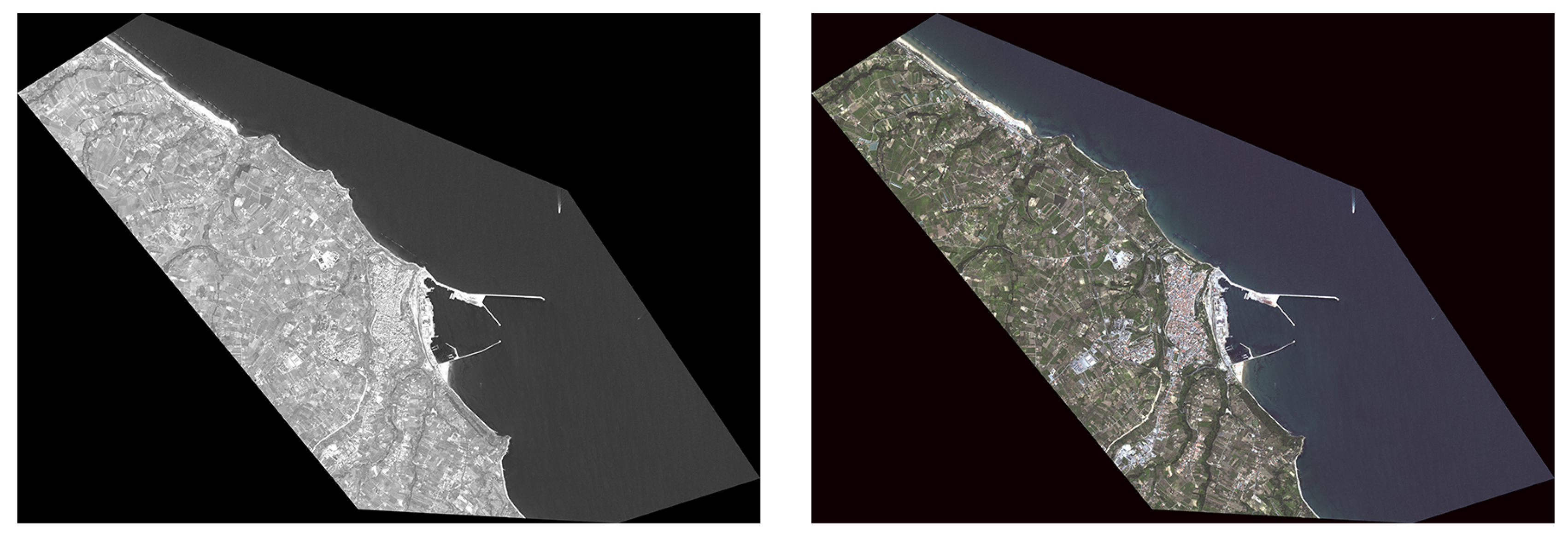
Figure 1. “Raw” WorldView-2 image: panchromatic (on the left) and multispectral (on the right).
Geosciences 09 00123 g001
Figure 2. Results of the decorrelation stretch of the entire image (on the left) and its detail (on the right).
Geosciences 09 00123 g002
Figure 3. NDVI on the entire image (on the left) and its detail (on the right).
Geosciences 09 00123 g003
Figure 4. World View Water Index (WVWI) on the entire image (on the left) and its detail (on the right).
Geosciences 09 00123 g004
Figure 5. Unsupervised classification (on the left) and supervised classification (on the right).
Geosciences 09 00123 g005
Figure 6. The I ( u i j ) neighborhood of an example image with radius = 1 and the relevant connections.
Geosciences 09 00123 g006
Figure 7. NDVI image (a), WVWI image (b), and application of CM on the NIR2 band image (c).
Geosciences 09 00123 g007
Figure 8. Profiles over three sample distances on the pansharpened image: Profile 1 is blue, Profile 2 green, and Profile 3 red.
Geosciences 09 00123 g008
Figure 9. Profiles over three sample distances on: NDVI (ac), WVWI (df) and CM over NIR2 image (gi). A, B and C, D are respectively referred to the shoreline extracted from the pansharpened image, used as reference, the artificial rocks and the shoreline extracted from NDVI, WVWI and CM algorithms.
Geosciences 09 00123 g009
Table 1. Shoreline changes between 1950/1999 and 2000/2007 [1,2].
1950/1999
Variations >±25 m
2000/2007
Variations >±5 m
Low-lying coastalkm%km%
Total4862100.04715100.0
Stable238749.1273758.0
Modified222745.8174437.0
Undefined2485.12345.0
Modified222745.8174437.0
Backwardness117024.189519.0
Progress105821.884918.0
Table 2. Differences between the reference images and the other filters at the shoreline (m).
NDVIWVWICM_NIR2
Profile 1 0.70 0.70 0.70
Profile 2Not well defined 0.40 0.33
Profile 31.00Not well defined 0.65