Article

ClimateDT: A Global Scale-Free Dynamic Downscaling Portal for Historic and Future Climate Data

1
CNR—Institute of Biosciences and BioResources, Florence Research Area, Via Madonna del Piano 10, I-50019 Sesto Fiorentino, Italy
2
Centre for Forest Management, Forest Research (FR), Roslin EH25 9SY, Midlothian, UK
*
Author to whom correspondence should be addressed.
Environments 2024, 11(4), 82; https://doi.org/10.3390/environments11040082
Submission received: 23 February 2024 / Revised: 10 April 2024 / Accepted: 15 April 2024 / Published: 17 April 2024

Abstract

:
Statistical downscaling of climate data has been widely described in the literature, with the aim of improving the reliability of local climatic parameters from coarse-resolution (often >20 km) global datasets. In this article, we present ClimateDT, a dynamic downscaling web tool for monthly historical and future time series at a global scale. The core of ClimateDT is the 1 km 1981–2010 climatology from CHELSA Climate (version 2.1), where the CRU-TS layers for the period 1901-current are overlayed to generate a historic time series. ClimateDT also provides future scenarios from CMIP5 using UKCP18 projections (rcp2.6 and rcp8.5) and CMIP6 using 5 GCMs, also available on the CHELSA website. The system can downscale the grids using a dynamic approach (scale-free) by computing a local environmental lapse rate for each location as an adjustment for spatial interpolation. Local predictions of temperature and precipitation obtained by ClimateDT were compared with climate time series assembled from 12,000 meteorological stations, and the Mean Absolute Error (MAE) and the explained variance (R2) were used as indicators of performance. The average MAEs for monthly values on the whole temporal scale (1901–2022) were around 1.26 °C for the maximum monthly temperature, 0.80 °C for the average monthly temperature, and 1.32 °C for the minimum monthly temperature. Regarding monthly total precipitation, the average MAE was 19 mm. As for the proportion of variance explained, average R2 values were always greater than 0.95 for temperatures and around 0.70 for precipitation due to the different degrees of temporal autocorrelation of precipitation data across time and space, which makes the estimation more complex. The elevation adjustment resulted in very accurate estimates in mountainous regions and areas with complex topography and substantially improved the local climatic parameter estimations in the downscaling process. Since its first release in November 2022, more than 1300 submissions have been processed. It takes less than 2 min to calculate 45 locations and around 8 min for the full dataset (512 records).

1. Introduction

Reliable and unbiased estimations of climatic variables for environmental assessments are fundamental in many research fields, including plant studies and forest sciences [1,2,3]. The climate is one of the key drivers shaping the distribution of living organisms across the globe [4,5,6]. In tree species, it forces the adaptive processes through time [7,8,9] and governs the future distribution of forest tree species worldwide [10,11,12]. The scientific community agrees that the shift of climatic normal parameters toward drier and warmer regimes, as well as the increased frequency of extreme weather events, will play a fundamental role in the future [13,14]. For such reasons, researchers call for more detailed climatological data to describe the environments where organisms grow as well as the ecological niche of studied species [12,13,14]. These data are required to model and forecast the possible consequences of a warming climate and potential adaptation strategies.
Interpolation techniques and downscaling methods have become relevant techniques used to generate climatological surfaces or to improve the quality and reliability of low-resolution climatic data [15,16,17,18,19,20,21,22]. Many different algorithms have been developed, linking the environmental variability and physiographic parameters, such as elevation or distance from the sea, applied to “delta” approaches [23] and statistical procedures [18,21,24,25,26]. Powerful workstations and tuned algorithms are readily accessible for research groups, often used in a statistical environment to predict the potential impact of a warming (and drying) climate on animals or plants [27,28]. In this context, the past climate is used to analyze the species’ responses to climate fluctuations [29,30], while the future scenarios are applied to forecast the possible impacts.
The reconstruction of past climates, such as paleoclimates and historical climates (e.g., from 1900 to the current periods) as a climate surface, is often performed by means of spatial interpolation. Amongst the most well-known techniques, Gaussian processes such as kriging (simple, ordinary, and universal) and co-kriging are often cited [31,32,33]. More recently, regression-based methods have proved useful, especially when large portions of geographic space are targeted. Amongst these methods, the PRISM surfaces available for North America [34] and WorldClim for the Globe [35,36] are well-known climatic data sources. For global surfaces, complex and time-consuming mechanistic downscaling algorithms were used to characterize the CHELSA-climate dataset [37]. However, the quality of the data is dependent on the spatial representativeness of the environment where interpolation is performed. Meteorological stations are spread globally, but the harmonization of their data is difficult [38,39]. Combined with historical climates, future scenarios are an additional requirement for modeling work. Climate change projections are driven by atmospheric processes and physical interactions constrained in mathematical models. Global Circulation Models (GCM), regularly developed by atmospheric scientists worldwide, are not targeted at specific geographic regions. According to recent literature, the projections generated by the IPCC 5th Assessment Report (AR5, CMIP5) are the most often used. However, CMIP6 [39,40] standard projections will probably replace AR5 in the coming decades. Such models generally have a low spatial resolution (more than 50 km at the equator) and are consequently unsuitable for national and regional studies. In this framework, spatial downscaling and statistical downscaling methods are common techniques used to improve the spatial resolution (and reliability) of coarse climatic surfaces [18,21]. Among all the available methods, the “delta method” and the “dynamic downscaling” [18,26,41] approaches (i.e., location by location, pixel by pixel) are popular among researchers requiring flexibility and ease of implementation in programming languages.
In this study, we present ClimateDT (https://www.ibbr.cnr.it/climate-dt, accessed on 17 January 2024), a web-based downscaling tool using a unique global climate extent that can be requested to deliver climate parameters from the same data for spatial consistency. Here, we describe the system for Europe, with an extension currently being developed for the United States, Canada, China, and other regions of the Globe. The seamless link between historical and future climate ensemble that researchers dealing with climate futures require is demonstrated, and the quality of climatological data provided by ClimateDT is evaluated against weather observations collected from external databases. Additionally, the speed of the system and its internal structure are described.

2. Materials and Methods

ClimateDT is an online tool with an R-based [42] computation engine that combines raster layers at various spatial scales and from different data sources. This structure has been created for both historical climate reconstruction and future scenarios at a monthly timescale. Here, a detailed description of its structure and workflow is given, covering all its features.

2.1. Baseline Surface: CHELSA 2.1 (1981–2010)

When long-term climate is used as a predictor variable in modeling work, climatic normals are used to describe the environmental variability and avoid the impact of weather fluctuations (i.e., year-by-year variability) on algorithm training. A climatic normal period represents the average climate over a reference period (series), usually spanning 10–30 years. Several climatological time series have been used in the literature. The 1961–1990 period is often considered a baseline in many biological and ecological studies [22,41] due to the large availability of climate data from the global network of stations [38]. The 1961–1990 climate series is also the backbone of ClimateWNA, ClimateNA [24], ClimateSA [26], ClimateEU [25], ClimateAP [26] (available at https://sites.ualberta.ca/~ahamann/data.html, accessed on 17 January 2024) and at https://web.climateap.net, accessed on 17 January 2024), and many other WorldClim-based studies and tools. However, the current climatic period (1991–2020) is rapidly diverging from the 1961–1990 climatic series, and for this reason, other datasets have been generated by climatologists. In ClimateDT, the 1 km 1981–2010 climate time series from CHELSA (v2.1) was selected as the baseline data [37] due to its global coverage and its acknowledged accuracy. The baseline data was used to seamlessly bind historical and future climates by calculating the deviations (i.e., anomalies) for the historic normal period and applying the anomalies to reconstruct the historical climate (1901-current) and future climate scenarios.

2.2. Historical Climate: CRU-TS

CRU-TS version 4.06 [38] is a monthly and global spatial dataset freely available from the Climatic Research Unit repository (http://www.cru.uea.ac.uk/data, accessed on 17 January 2024) which provides monthly maximum and minimum temperature as well as precipitation between 1901 and the current year. This database has been widely used for downscaling and data extraction [24] and is the main source for many research studies where monthly time series are required [43,44,45]. The native spatial resolution (0.5° degrees of latitude, approximately 50 km at the equator) is too coarse for national and regional studies, especially in areas of complex terrain. ClimateDT employs this dataset to generate higher-resolution historical climate data time series based on the anomalies concept. The 1981–2010 normal period is calculated within CRU-TS surfaces, averaging the layers with monthly resolution and generating 36 new global raster layers at 50 km spatial resolution. Anomalies are derived from the 1981–2010 baseline period using the difference in temperature and the ratio for precipitation according to method described by Moreno and Hasenauer [23]. The effect of elevation and terrain features on anomalies are considered after the downscaling process [46], and these are stored and downscaled dynamically by ClimateDT to 1 km using bilinear interpolation to match the baseline’s spatial resolution.

2.3. CMIP5 and CMIP6 Future Scenarios

A fundamental feature of a climatological portal or tool is the provision of consistent historical data and future scenarios, allowing users to apply ecological models and algorithms that more accurately predict the likely effects of the changing climate on the environment and ecosystems. While many datasets are available on the web, most are not interchangeable. For example, WorldClim surfaces [35,36] are different and not directly compatible with CHELSA products [37]. Although both services can provide future scenarios (both CMIP5 and CMIP6), admixing the two sources can generate unknown biases in the models due to different interpolation methods or different baselines used to calculate anomalies.
Since researchers often need an ensemble of GCMs to investigate the variability between and within GCMs [47,48,49] and climate change emissions scenarios, i.e., Representative Concentration Pathways (RCPs) from CMIP5 and Shared Socio-Economic Pathways (SSPs) from CMIP6, both have been implemented in ClimateDT. ClimateDT provides future scenarios under the Fifth Assessment Report [50] using the UKCP Global dataset [51], a monthly, global, low-resolution (60 km approx.) dataset spanning the period from December 1899 to November 2099, and UKCP Regional (12 km) projections with a monthly time series from 1981 to 2080 for Europe. These datasets use cutting-edge climate science to provide updated observations and global (and European) climate change projections. In ClimateDT, this database was analyzed for the 1981–2010 climatic normal period in the same way as CRU-TS—using the anomalies approach. The climate change forcing (anomaly) was calculated from the common normal period and added to the baseline period data using bilinear interpolation. This procedure removes the intrinsic difference between the two datasets to generate a unique and robust time series between 1901 and 2098. All 28 UKCP Global ensemble members (i.e., variations form the HAdGEM3 model) are available in ClimateDT for the two RCP extreme scenarios (2.6 and 8.5). Since CMIP6 scenarios were not available as a time series with the 1981–2010 baseline, only the CMIP5 data linked to the climatic normal using the CHELSA data were included in ClimateDT for consistency.

2.4. Scale-Free Dynamic Downscaling

The core of ClimateDT is based on dynamic downscaling proposed by Wang et al. for North America [46]. This method combines the use of a plane spatial interpolation (usually a bilinear interpolation) and local lapse rate adjustment to refine the climate parameter for a specific spatial location (point estimate, scale-free). The adjustment is based on the spatial coordinate of the location requested. This approach forms the core of other standalone tools, such as ClimateWNA for North America, [24,52], ClimateAP for Asia [26], and ClimateEU for Europe [25].
Following the submission of a data request in the ClimateDT portal, where latitude, longitude, and elevation are mandatory fields, the downscaling process starts with the identification of the location of the 1 km grid cell stored in the remote ClimateDT machine. Afterward, each location is processed separately in four steps. The first computes the bilinear interpolation of the 36 basic climatic data (monthly minimum and maximum temperatures and total precipitation) for the baseline (i.e., the normal 1981–2010 climate), which is performed by means of a weighted interpolation of the climatic values the system extracts for the nearest 4 cells of the raster (Figure 1, left). The second step extracts the same 36 climatic variables for each of the 8 local grid cells surrounding the location plus the cell where the location falls (9 in total). A set of 36 unique pairs of differences (i.e., climate derived for the first cell versus all the others; then the same for cell 2, excluding cell 1; then cell 3; and so on), afterwards ∆c values are computed. The same procedure is applied to elevation data (∆e) for a total of 37 sets of data created by 36 unique pairs of differences each. After that, 36 simple linear regressions are built (Figure 2) based on the above 36 pairs plus the elevation set.
Δ c = i + m Δ e
This is performed to reflect the local relationship between ∆c and ∆e for each of the 36 climatic variables (i.e., how large the change is in degrees of temperature or millimetres of rain when a change in elevation occurs). The slope of the regression line m represents the local (i.e., dynamic) lapse rate for the raster cell where the point of interest is located. Both temperature and precipitation variables are adjusted using the dynamic lapse rates when the regression of temperature or precipitation variation in elevation for ’local’ grid cells of the spatial raster are statistically significant.
The difference between the actual elevation of the location and the spatially interpolated elevation of the point of interest is used in the equation and summed to the spatially interpolated value as
A d j u s t e d   c l i m a t e = S i n t + m · ( E i n t E u s e r ) · R 2
where Sint is the spatial interpolation of climatic variable, m is the local lapse rate, Eint is the elevation the system calculates from the 1 km Digital Elevation Model by means of bilinear interpolation (the same method as Sint), Euser is the elevation provided by the user in the submitted file, and R2 is the adjusted R-squared of the regression calculated using ∆c and ∆e values. Since elevation is required for ClimateDT, this information should be carefully checked by the user. Input data are used to calculate the difference (delta) between the reference elevation of the system (i.e., WorldClim DEM in ClimateDT) and the ‘real’ site elevation provided by the user. This delta is used for the dynamic lapse rate adjustment to be applied to the climatic value interpolated with the ‘flat’ bilinear interpolation.
It is worth mentioning that the dynamic downscaling procedure is applied to the 1981–2010 baseline period for the three main climatic parameters: monthly minimum temperature, monthly maximum temperature, and monthly precipitation. After that procedure is completed for all the locations, anomalies are spatially downscaled and summed (or subtracted/multiplied according to the sign of the numbers and of the target climatic parameters) to the dynamically downscaled baseline climate using the same bilinear interpolation process on a 50 km grid. Finally, the historic (1901-now) and the future (now-2098 for UKCP Global, climatic normals for CMIP6 GCMs) climate is ready.

2.5. Climatic Indices Calculation

Following the dynamic lapse rate adjustment on monthly variables, the full set of biologically relevant climate variables are either calculated (seasonal and annual summaries) or estimated (e.g., growing degree days and frost-free period) using a correlative approach with values derived from daily weather station data [24,25,26,52]. The main outputs of ClimateDT are three monthly variables (minimum temperature, maximum temperature, and precipitation) calculated for each year requested by the user. Additional climatic variables and indices (annual or monthly) over the whole time period can be calculated as well. Some of these parameters, such as the 19 bioclimatic parameters from WorldClim, are calculated using the “dismo” package in R [53], while SPEI and SPI indices are derived using the “SPEI” package [54]. The dismo package, an acronym for “species DIStribution MOdeling”, is an R package which includes several algorithms for modeling, such as DOMAIN, Mahalanobis distance, and MaxEnt, as well as functions to compute climatic indices. The package includes a set of functions for computing potential evapotranspiration and several widely used drought indices, including the Standardized Precipitation–Evapotranspiration Index (SPEI), which is employed in ClimateDT. Other drought and frost indices available in the literature and widely used in ClimateNA, ClimateAP, and ClimateEU systems can be calculated using simple equations, including Growing Degree Days above 0 °C, 5 °C, and 18 °C (GDD0, GDD5, and GDD18, respectively). The coefficients are derived by fitting a set of linear and nonlinear functions on observed daily meteorological station data from the European Climate Assessment and Dataset (ECAD, https://www.ecad.eu/, accessed on 17 January 2024) to calculate the derived climate variables and then building the relationship (or function) between the derived variables and the observed data. The resulting parameters allow ClimateDT to adjust the climate indices from downscaled monthly climate data and offer more accurate estimations of future climate.

2.6. Quality Assessment of ClimateDT Estimates

To validate ClimateDT parameter estimates, a quality assessment was carried out by comparing the observations obtained from various weather stations worldwide with climate variables generated by the downscaling tool. However, it is worth noting that all or most of the records included in the validation step may have been used for the development of interpolated climate grids CHELSA and CRU-TS, and this might represent a major though unsolvable limitation to the adopted approach. Therefore, our quality assessment could not use an independent validation test but rather an evaluation of how well ClimateDT reflects the real data and how the dynamic downscaling process could improve the reliability and quality of the climatic variables. We evaluated the benefits of the environmental lapse rate adjustments and the effectiveness of delta downscaling approach [24,25].
Prior to the quality assessment, we combined and filtered the datasets from the weather stations, retaining only those having climate time series exceeding 30 years of collected data and less than 10% of missing values. We also removed nearby duplicate stations by retaining only the highest-quality station records. Overall, approximately 12,000 weather stations for precipitation and 4000 for temperature were retrieved from the ECAD website. Only Europe and Russia were adequately covered (Figure 3) in the Northern Hemisphere.
Nonetheless, this dataset covers a wide range of ecological conditions and therefore was considered suitable to test the performance of ClimateDT both across altitudinal ranges (for the sea level up to 3500 m) and different climatic zones (from the Mediterranean Basin to the Boreal and Artic biogeographic zones). For these stations, we evaluated the performance of ClimateDT to describe the historical estimates (1901-current) based on the variance explained in original climate station data. The goodness-of-fit of a simple linear model between predicted and an observed climate value was assessed using its R2 and the Mean Absolute Error (MAE), i.e., the mean absolute difference (in °C for temperature and in mm for precipitation) between ClimateDT estimates and observed station data. This procedure is similar to published studies on ClimateEU and ClimateNA [24,25] with an additional analysis grouping climate station by country and showing the MAEs and R2 values for some locations in key geographic zones and climates (e.g., Mediterranean climate and continental climate).

3. Results

Climatic time series in the ECAD dataset were available from a larger number of weather stations since 1901, with a huge increment in the available data around the 1980s (Figure 4), especially for the precipitation data, which, however, had a higher proportion of missing data. Nonetheless, sufficient records with few missing data over the period 1901–1950 were also available for testing the performance of ClimateDT.
While the number of precipitation data stations registered a maximum value around 1990, with 12,357 records, but with a subsequent decrease (around 10 k in 2015), the temperature data steadily increased over the whole period. For the last 2 years of testing (2017 and 2018), the available records slightly decreased, probably due to missing data and a different release from ECAD.
The performance of ClimateDT was assessed using four main climatic variables, which represent the raw data used in the calculation of the climatological indices and include the maximum monthly temperature (TX), the average monthly temperature (TAVE), the minimum monthly temperature (TN), and the total monthly precipitation (RR). ClimateDT estimates for the four climatic parameters were tested against the values from meteorological stations at the same location both over the 1981–2010 baseline period and the whole 1901–2022 period. Regarding the baseline period (Table 1), the MAE for temperature ranged between 1.61 °C for the minimum temperature of May and 0.49 °C for the average temperature of September. Overall, the average MAE for monthly values was 1.24 °C for TX, 0.67 °C for TAVE, and 1.19 °C for TN. Regarding monthly total precipitation, MAE values were always lower than 12 mm, with an average of 9.46 mm and a maximum value of 11.68 mm in December. A shortcoming of MAE as an indicator is that it is impossible to detect whether ClimateDT’s predictions are higher or lower than the observed values, but the analysis of raw errors indicates that RR and TN were slightly overestimated, while TX and TAVE are underestimated. As for the proportion of variance explained, average R2 values were around 0.961, 0.968, and 0.918 for TX, TAVE, and TN, respectively. A slightly lower amount of explained variance was found for RR, with an average value of 0.850. The maximum value was detected in August (0.882), and the lowest was detected in April (0.820).
When the full temporal coverage (1901–2022) was considered (Table 2), the MAE for temperature was consistent to some extent with the previous results. The estimation error ranged between 1.59 °C for the maximum temperature of July and 0.60 °C for the average temperature of September. The average MAE for monthly values was 1.26, 0.80, and 1.32 °C for TX, TAVE, and TN, respectively. For precipitation, MAE values were higher than those calculated over the baseline period (average MAE = 19 mm). In agreement with the previous analysis, a slight overestimation was found for RR and TN over the normal 1981–2020 period, while values for TX and TAVE were slightly underestimated. R2 values showed average values of 0.960, 0.966, and 0.919 for TX, TAVE, and TN, respectively, which substantially corresponded to the results obtained from the comparison of predicted and observed values over the baseline period. Again, a lower amount of explained variance was found for RR, with an average value of 0.675; the highest value was in October (0.718), and the lowest was in July (0.621).
In general, the precision of climate predictions from ClimateDT increases with the length of time considered, e.g., TAVE annual estimates from Climate DT were more precise than seasonal variable estimates, which in turn were more precise than monthly variable estimates. Also, predictions for precipitation-related variables were generally less precise than those for temperature, likely due to the data gaps in the ECAD dataset. An overlap between explained variance and MAE is graphically shown in Figure 5 for some key months.
The assessment of MAEs and R2 values at the regional scale showed that the performance of ClimateDT was almost stable in all the climates and at any geographic scale (Table 3).

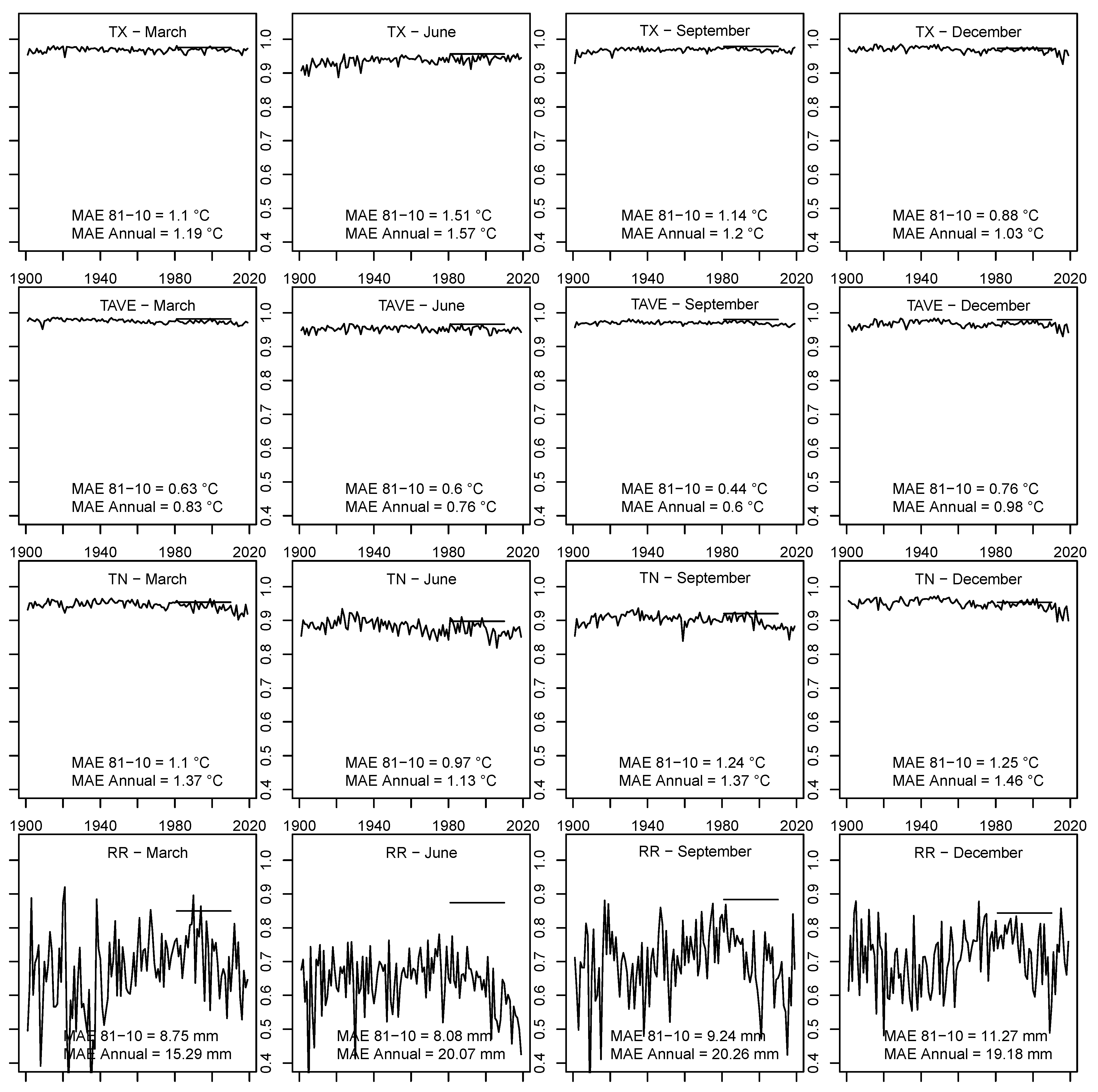
3.1. Effectiveness of the Dynamic Lapse-Rate Adjustment

The main feature of ClimateDT is the dynamic downscaling approach to the gridded baseline data to generate scale-free climate predictions at a global level. The lapse-rate adjustments are shown to be effective by comparing the MAE observed with and without adjustment in mountainous areas and in cases of complex topography. As expected, MAEs of climate estimates were higher for climate values directly obtained for mountainous areas, with lapse rate adjustments for temperature-related variables ranging between −0.40 and −0.67 °C every 100 m of elevational shift. This adjustment substantially improved the quality of climate estimates in mountainous regions, resulting in an average decrease in MAE between −0.20 and −0.50 °C, which represents an improvement of up to 65%. The effectiveness of the adjustment was more noticeable for TX and TAVE, while improvements were relatively minor for TN.
The adjustment for precipitation-related variables was observed to be more difficult because of the weaker relationship between rainfall and elevation. Despite that, and in contrast to climatic software such as ClimateEU (v4.63) and ClimateNA (v6.40a), the lapse rate adjustment for precipitation was filtered and applied only in the case of significant fitting of the regression of climate parameters to elevation. This results in a fairly low but still meaningful improvement in ClimateDT estimates, with the lapse rate adjustment having an impact of about −5% of MAE on precipitation estimates.
The second metric used for assessing the performance of ClimateDT, i.e., the proportion of variance explained (R2), also supports the effectiveness of the dynamic lapse rate adjustment to obtain more accurate and reliable values of the climatic variables considered in mountainous terrains. Indeed, a substantial difference in the accuracy of monthly precipitation and temperature estimates was detected, with R2 increased by +20% in some cases. Overall, non-adjusted predictions showed average R2 values of about 0.85, whereas the adjustment improved the R2 up to 0.95–0.97. Finally, the effectiveness of the lapse rate adjustment was more important for TAVE and TX than for TN and RR during the summer months.

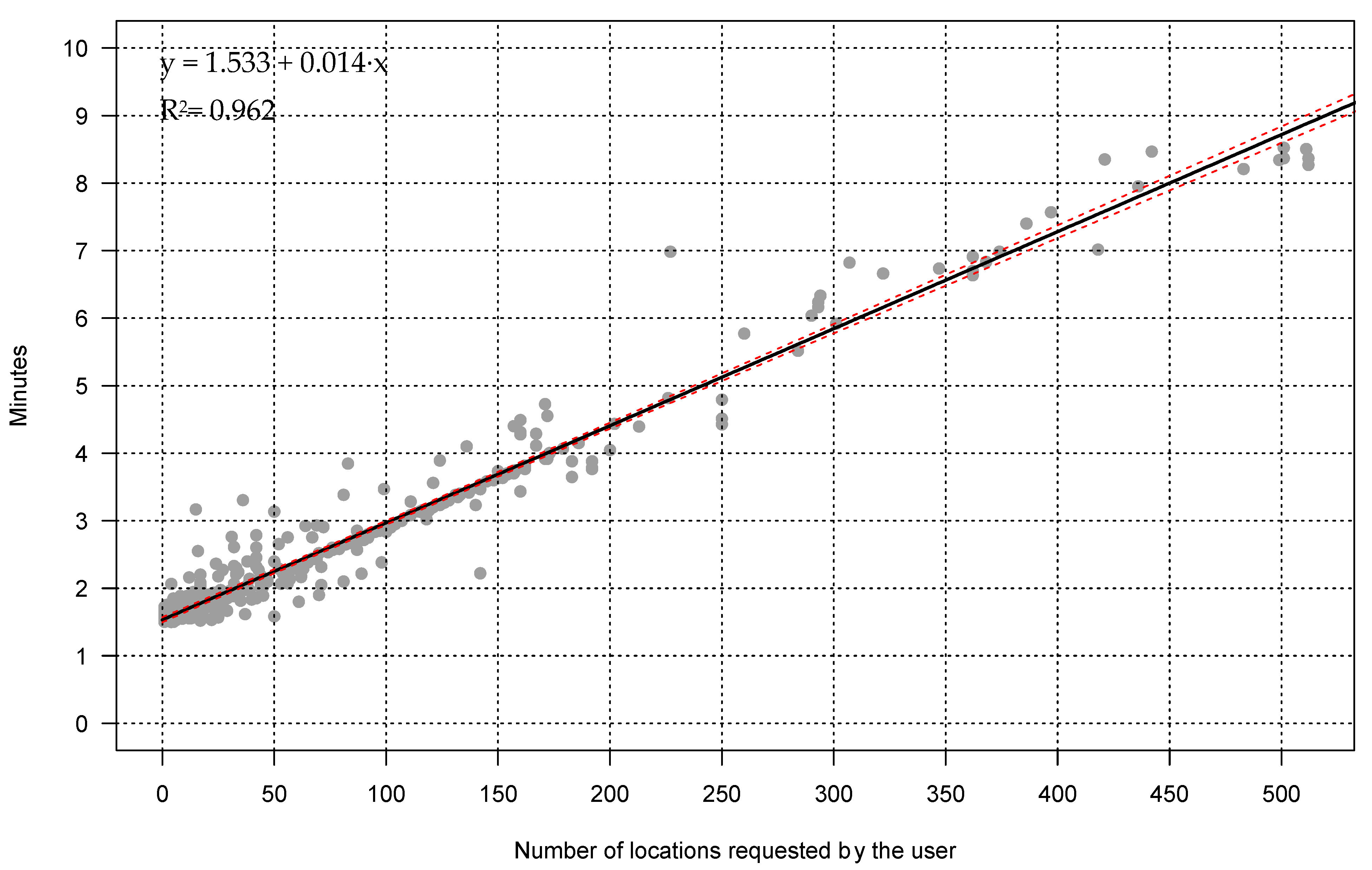
3.2. Requests Counter and Processing Rate

Since its release in November 2022, a total of 1321 submissions (updated February 2024) were processed and downscaled, with an overall number of locations successfully processed equal to 165,869 (130.6 ± 195.4 locations per request, on average). Currently, the ClimateDT tool employs a parallelization of the R code on 3 CPUs with a Xeon processor on a shared server. The performance of this hardware configuration is shown in Figure 6.
Less than 2 min was necessary to calculate the full set of climatic parameters at 45 locations and around 9 min was necessary for the maximum number of localities that can be requested (512 records). We acknowledge a relatively high fluctuation in terms of processing rate, and this was due to other simultaneous processes running on the CPUs (e.g., system updates and other tasks internal to the Operating System). More than 65% of requests were characterized by a low number of records (less than 50), and only 3% were requests for large coverage, which has been limited for internal needs to 512 locations per submission. Almost all of the submissions requested full temporal coverage (1901–2098), and most selected the standard GCM (variant01) and rcp8.5. Several users have repeated their submissions for the same locations to obtain local climatic estimates under different future scenarios. In this case, a total of 5 GCMs was the most frequent request by the same user. Most of the requests were submitted from all the European countries, but more recently, they have also been from Asian countries, North America and Africa, representing altogether 18% of the total submissions.

4. Discussion

ClimateDT can be used for downscaling various raw climatic parameters and indices between 1901 and 2098. This tool incorporates three different sources of climatic data: a high-resolution grid as a baseline for the normal period of 1981–2010, a dataset of monthly anomalies for the historical climate derived from CRU-TS, and future scenarios from UKCP Global surfaces. Input data are spatial coordinates and elevation used in the scale-free statistical downscaling procedure. The system has global coverage, and the speed of analysis is currently comparable to other available resources, such as ClimateEU, ClimateNA, and ClimateAP [24,25,26,41]. Small differences in MAE values were found when compared against ClimateEU, likely due to the different climate time series used for evaluation or validation. A large- number of weather stations were used for ClimateDT, and a large spatial coverage was also provided. The evaluation process demonstrated a weak effect of the dynamic lapse rate adjustment for the minimum temperature. This was also found in other case studies [24,25,41], likely due to the occurrence of temperature inversions that make it difficult to derive reliable lapse rates. For ClimateDT, this effect was limited and probably fixed in most cases due to the use of CHELSA surfaces as the baseline, which is known to capture such climatological effects in the spatial pattern resulting from the method climatologists have used to generate CHELSA layers [37].
After decades of research on the possible climate change impacts on plants and forest resources associated with a changing climate [55,56,57,58,59], many of the geographic regions in the world have been studied. Published research includes efforts on various aspects such as retrospective analysis [44,60,61], statistical models [62,63], and various spatial modeling techniques across different species [64,65,66]. In general, reliable climatic surfaces are important for prediction, and databases to train models have been stressed as an important added value to climate-related studies [48,67,68]. An important strength of ClimateDT is the use of a unique surface at the global level that provides consistent results across the whole globe. The admixing of different climatic data sources, such as PRISM surfaces in the case of ClimateNA for North America [34], WorldClim surfaces for ClimateEU in Europe [35,69], and other datasets around the globe [26,41,70], may introduce biases in the calculation of statistical models and could affect predictions [48,71]. In this context, the use of a unique baseline deployed by ClimateDT represents a novel and standardized approach in that both historical climate and future scenarios are placed as anomalies. In addition, the realization of a web portal instead of an app or software to be installed on client operating systems reduces the system requirements on the end-user side. Further, updates in the ClimateDT tool are applied on the server side automatically. For example, every time a new surface is released by climatologists (e.g., new CRU-TS layers), it is easily incorporated into the system and made immediately available to users. Finally, ClimateDT relies on a quality check against the Google Map™ APIs for spatial coordinates, elevation, and data consistency before submission. This also improves the usability of the system and ensures a proficient and efficient tool with an R code engine at the core. This results in a quick and user-friendly system available for users worldwide.

4.1. Usage of ClimateDT and Potential Benefits of Its Estimates

The validation process stresses the importance of accurate geographic input data for downscaling. The availability of the large number of records included in the ECAD allowed us to test the downscaling system over a large range of different environments. Several attempts were made to compensate for the missing values in the dataset, to complete the missing information (mainly elevation data), and to check the spatial coordinates. On average, most records were provided with minutes of latitude, and elevation was often rounded to 50 m. This creates spatial uncertainty in the location of weather stations of about 2 km, which can drastically affect the downscaling process in mountainous areas. ClimateDT can adjust input data with user approval by means of external datasets (e.g., extracting the elevation from a high-resolution DEM) since the need for precise coordinates is mandatory in the process. On average, ClimateDT calculates a lapse rate range between −0.4 °C/100 m and −0.6 °C/100 m of elevation, which is fully consistent with the MAE obtained during the validation process. The reliability of spatial coordinates has been acknowledged as a key component in the ClimateDT functioning, and users are highly encouraged to check the input data very carefully to obtain unbiased values. The need for reliable coordinates has been helped by using an overlay with Google Maps™ to check the input data before submission.
The use of tailored downscaled data and climatological indices (more than 80 in ClimateDT) can allow researchers to develop an ecological modeling procedure faster and easier. One of the main outputs of ecological models such as Species Distribution Models [72], Joint Species Distribution Models [73,74], reaction norms [28,30], response functions [71,75,76,77], and transfer models [27,78] is the prediction of the possible changes in the spatial distribution and/or the performance of living organisms under changing climatic regimes. An additional feature is to detect provenances that may show better adaptation to the future climate predicted in a specific area [79,80,81]. Such models may be used as valid tools to support assisted gene-flow and assisted-migration strategies, but their performance is highly dependent on the quality of the climatic information used to drive the model and to make predictions [81,82]. The higher the uncertainty in the modeling steps, the more uncertain and biased the predictions could be. In this case, the probability of failure is proportional to the discrepancy between the climate forecasted by the models and the actual climate occurring in the future at a specific location. The main modeling issues associated with future projections could be represented by errors or bias occurring in the spatial interpolation of climatic variables; the use of inappropriate equations to calculate daily derived indices from monthly data, e.g., the Number of Frost-Free Days (NFFD), Growing Degree Days (GDD); and other biologically relevant indices. Therefore, according to the literature, an uncertainty assessment is fundamental in any modeling step [27,83,84,85,86].

4.2. Raster Surfaces Availability and Consistency with CHELSA Layers

ClimateDT has been developed to generate scale-free climatological variables for multiple locations around the world, though their number is currently limited to 512 per submission. The pre-check of the requested locations before submission is based on Google Maps™ APIs and prevents the downscaling system from failure and/or unexpected bugs due to misleading coordinates or elevation data. However, applying the above limit allows the submission of only 10% of the potential usage of the system. The reason for maintaining a limit to submitted locations is to allow multiple submissions in parallel and to deliver faster results. Our evidence shows that the overlocked version of ClimateDT can process up to 10,000 locations per submission, which leaves large room for future improvement to the system. However, increasing the current site limit per submission would commit the downscaling tool to processing a single request for several hours, with the possible consequence of long queues. For this reason, submissions of a larger number of records/localities are possible upon request but will be handled separately through the application. Indeed, future hardware improvements (number of cores, solid state storage, etc.) are expected to speed up the downscaling process, allowing for a larger number of localities per submission and reduced processing time.
While point estimates are an excellent source used to derive the climate of origin of provenances tested in common garden experiments [71,87] or to derive the fundamental niche of forest tree species based on occurrence data [88,89], spatial data surfaces are necessary to make spatial predictions [90,91]. In this context, it is worth mentioning that ClimateDT estimates are fully compatible with any global layer available in the CHELSA repository, where the 1981–2010 baseline is available at a 1 km spatial resolution, as well as future scenarios under CMIP6. Users can therefore run the models on the climate obtained from ClimateDT (point estimates) and make predictions on the CHELSA layers. Finally, new downscaled raster surfaces with higher spatial resolution for specific areas may be released on the ClimateDT portal. Several case studies in Italy have produced maps at a 250 m resolution [17,28], including the most recent normal 1991–2020 climate and several future scenarios.

5. Conclusions

ClimateDT is an open-source web tool that is continuously being developed. Users can submit the geographic coordinates of their study locations through the web interface without any registration by simply providing a valid email address. The system processes the locations and returns by e-mail- a link where the downscaled dataset can be downloaded, along with a short report summarizing the downscaling results. New indices, interpolation methods, baselines, historical and future datasets, and tools are planned to be included in the system in future releases. The possibility of an additional section of the ClimateDT portal to request raster surfaces is also under development, as well as the implementation of additional features using new packages provided by other researchers/developers in R language. Any additional feedback from users is welcome, and new ideas and needs can be sent to the staff to implement new indices currently missing in the ClimateDT output files.

Author Contributions

Conceptualization, M.M. and D.R.; methodology, M.M, G.B. and D.R.; software, M.M., G.B., P.I. and D.R.; formal analysis, P.I.; investigation, G.B. and D.R.; resources, G.B. and D.R.; data curation, M.M. and P.I.; writing—original draft preparation, M.M. and D.R.; writing—review and editing, M.M., G.B., P.I. and D.R.; project administration, D.R.; funding acquisition, M.M. and D.R. All authors have read and agreed to the published version of the manuscript.

Funding

The ClimateDT conceptualization and realization was funded by the EU in the framework of the Horizon 2020 B4EST project “Adaptive BREEDING for productive, sustainable and resilient FORESTs under climate change”, UE Grant Agreement 773383. M.M., G.B. and P.I. were also partially funded by the project IR0000032—ITINERIS, Italian Integrated Environmental Research Infrastructures System—CUP B53C22002150006 (D.D. n. 130/2022) Funded by the EU—Next Generation EU—Mission 4 “Education and Research”—Component 2: “From research to business”—Investment 3.1: “Fund for the realisation of an integrated system of research and innovation infrastructures” and by the PRIN2022—CONIFIR project “GenetiC Origin and structural setting of douglas-fir plaNted forests in Italy For their management, conservatIon and valoRization”, project number DBA.PN011.009, CUP B53D23015090006.

Data Availability Statement

The original contributions presented in the study are included in the article, further inquiries can be directed to the corresponding author.

Conflicts of Interest

The authors declare no conflicts of interest.

References

  1. Bärring, L.; Berlin, M.; Andersson Gull, B. Tailored Climate Indices for Climate-Proofing Operational Forestry Applications in Sweden and Finland. Int. J. Climatol. 2017, 37, 123–142. [Google Scholar] [CrossRef]
  2. Perdinan, P.; Winkler, J.A. Changing Human Landscapes under a Changing Climate: Considerations for Climate Assessments. Environ. Manag. 2014, 53, 42–54. [Google Scholar] [CrossRef] [PubMed]
  3. Fady, B.; Esposito, E.; Abulaila, K.; Aleksic, J.M.; Alia, R.; Alizoti, P.; Apostol, E.-N.; Aravanopoulos, P.; Ballian, D.; Kharrat, M.B.D.; et al. Forest Genetics Research in the Mediterranean Basin: Bibliometric Analysis, Knowledge Gaps, and Perspectives. Curr. For. Rep. 2022, 8, 277–298. [Google Scholar] [CrossRef]
  4. Franklin, J.; Davis, F.W.; Ikegami, M.; Syphard, A.D.; Flint, L.E.; Flint, A.L.; Hannah, L. Modeling Plant Species Distributions under Future Climates: How Fine Scale Do Climate Projections Need to Be? Glob. Chang. Biol. 2013, 19, 473–483. [Google Scholar] [CrossRef]
  5. Sinclair, S.J.; White, M.D.; Newell, G.R. How Useful Are Species Distribution Models for Managing Biodiversity under Future Climates? Ecol. Soc. 2010, 15, 8. [Google Scholar] [CrossRef]
  6. Araújo, M.; Pearson, R.; Rahbek, C. Equilibrium of Species’ Distribution with Climate. Ecography 2005, 28, 693–695. [Google Scholar] [CrossRef]
  7. Hamann, A.; Roberts, D.R.; Barber, Q.E.; Carroll, C.; Nielsen, S.E. Velocity of Climate Change Algorithms for Guiding Conservation and Management. Glob. Chang. Biol. 2015, 21, 997–1004. [Google Scholar] [CrossRef] [PubMed]
  8. Carroll, C.; Roberts, D.R.; Michalak, J.L.; Lawler, J.J.; Nielsen, S.E.; Stralberg, D.; Hamann, A.; Mcrae, B.H.; Wang, T. Scale-Dependent Complementarity of Climatic Velocity and Environmental Diversity for Identifying Priority Areas for Conservation under Climate Change. Glob. Chang. Biol. 2017, 23, 4508–4520. [Google Scholar] [CrossRef] [PubMed]
  9. Picard, N.; Marchi, M.; Serra-Varela, M.J.; Westergren, M.; Cavers, S.; Notivol, E.; Piotti, A.; Alizoti, P.; Bozzano, M.; González-Martínez, S.C.; et al. Marginality Indices for Biodiversity Conservation in Forest Trees. Ecol. Indic. 2022, 143, 109367. [Google Scholar] [CrossRef]
  10. Stürck, J.; Poortinga, A.; Verburg, P.H. Mapping Ecosystem Services: The Supply and Demand of Flood Regulation Services in Europe. Ecol. Indic. 2014, 38, 198–211. [Google Scholar] [CrossRef]
  11. Hamann, A.; Wang, T. Potential Effects of Climate Change on Ecosystem. Ecology 2006, 87, 2773–2786. [Google Scholar] [CrossRef] [PubMed]
  12. Fleischer, P.; Pichler, V.; Flaischer, P.; Holko, L.; Mális, F.; Gömöryová, E.; Cudlín, P.; Holeksa, J.; Michalová, Z.; Homolová, Z.; et al. Forest Ecosystem Services Affected by Natural Disturbances, Climate and Land-Use Changes in the Tatra Mountains. Clim. Res. 2017, 73, 57–71. [Google Scholar] [CrossRef]
  13. Ummenhofer, C.C.; Meehl, G.A. Extreme Weather and Climate Events with Ecological Relevance—A Review. Philos. Trans. R. Soc. B: Biol. Sci. 2017, 372, 20160135. [Google Scholar] [CrossRef] [PubMed]
  14. Barros, C.; Guéguen, M.; Douzet, R.; Carboni, M.; Boulangeat, I.; Zimmermann, N.E.; Munkemuller, T.; Thuiller, W. Extreme Climate Events Counteract the Effects of Climate and Land-Use Changes in Alpine Tree Lines. J. Appl. Ecol. 2017, 54, 39–50. [Google Scholar] [CrossRef] [PubMed]
  15. Paniccia, C.; Di Febbraro, M.; Frate, L.; Sallustio, L.; Santopuoli, G.; Altea, T.; Posillico, M.; Marchetti, M.; Loy, A. Effect of Imperfect Detection on the Estimation of Niche Overlap between Two Forest Dormice. IForest 2018, 11, 482–490. [Google Scholar] [CrossRef]
  16. Thuiller, W.; Lavorel, S.; Sykes, M.T.; Araújo, M.B. Using Niche-Based Modelling to Assess the Impact of Climate Change on Tree Functional Diversity in Europe. Divers. Distrib. 2006, 12, 49–60. [Google Scholar] [CrossRef]
  17. Corona, P.; Bergante, S.; Marchi, M.; Barbetti, R. Quantifying the Potential of Hybrid Poplar Plantation Expansion: An Application of Land Suitability Using an Expert-Based Fuzzy Logic Approach. New For. 2024. [Google Scholar] [CrossRef]
  18. Tang, J.; Niu, X.; Wang, S.; Gao, H.; Wang, X.; Wu, J. Statistical Downscaling and Dynamical Downscaling of Regional Climate in China: Present Climate Evaluations and Future Climate Projections. J. Geophys. Res. Atmos. 2016, 121, 2110–2129. [Google Scholar] [CrossRef]
  19. Flint, L.E.; Flint, A.L. Downscaling Future Climate Scenarios to Fine Scales for Hydrologic and Ecological Modeling and Analysis. Ecol. Process. 2012, 1, 2. [Google Scholar] [CrossRef]
  20. Moriondo, M.; Bindi, M. Comparison of Temperatures Simulated by GCMs, RCMs and Statistical Downscaling: Potential Application in Studies of Future Crop Development. Clim. Res. 2006, 30, 149–160. [Google Scholar] [CrossRef]
  21. De Cáceres, M.; Martin-StPaul, N.; Turco, M.; Cabon, A.; Granda, V. Estimating Daily Meteorological Data and Downscaling Climate Models over Landscapes. Environ. Model. Softw. 2018, 108, 186–196. [Google Scholar] [CrossRef]
  22. Liu, S.; Liang, X.; Gao, W.; Stohlgren, T.J. Regional Climate Model Downscaling May Improve the Prediction of Alien Plant Species Distributions. Front. Earth Sci. 2014, 8, 457–471. [Google Scholar] [CrossRef]
  23. Moreno, A.; Hasenauer, H. Spatial Downscaling of European Climate Data. Int. J. Climatol. 2016, 36, 1444–1458. [Google Scholar] [CrossRef]
  24. Wang, T.; Hamann, A.; Spittlehouse, D.; Carroll, C. Locally Downscaled and Spatially Customizable Climate Data for Historical and Future Periods for North America. PLoS ONE 2016, 11, e0156720. [Google Scholar] [CrossRef] [PubMed]
  25. Marchi, M.; Castellanos-acuña, D.; Hamann, A.; Wang, T.; Ray, D.; Menzel, A. ClimateEU, Scale-Free Climate Normals, Historical Time Series, and Future Projections for Europe. Sci. Data 2020, 7, 428. [Google Scholar] [CrossRef] [PubMed]
  26. Wang, T.; Wang, G.; Innes, J.L.; Seely, B.; Chen, B. ClimateAP: An Application for Dynamic Local Downscaling of Historical and Future Climate Data in Asia Pacific. Front. Agric. Sci. Eng. 2017, 4, 448–458. [Google Scholar] [CrossRef]
  27. Hallingbäck, H.R.; Burton, V.; Vizcaíno-palomar, N.; Trotter, F.; Liziniewicz, M.; Marchi, M.; Berlin, M.; Ray, D.; Benito-Garzón, M. Managing Uncertainty in Scots Pine Range-Wide Adaptation under Climate Change. Front. Ecol. Evol. 2021, 9, 724051. [Google Scholar] [CrossRef]
  28. Marchi, M.; Bergante, S.; Ray, D.; Barbetti, R.; Facciotto, G.; Chiarabaglio, P.M.; Hynynen, J.; Nervo, G. Universal Reaction Norms for the Sustainable Cultivation of Hybrid Poplar Clones under Climate Change in Italy. IForest 2022, 15, 47–55. [Google Scholar] [CrossRef]
  29. Booth, T.H. Assessing Species Climatic Requirements beyond the Realized Niche: Some Lessons Mainly from Tree Species Distribution Modelling. Clim. Chang. 2017, 145, 259–271. [Google Scholar] [CrossRef]
  30. Benito Garzón, M. Phenotypic Integration Approaches Predict a Decrease of Reproduction Rates of Caribbean Pine Populations in Dry Tropical Areas. Ann. For. Sci. 2021, 78, 69. [Google Scholar] [CrossRef]
  31. Hartkamp, A.D.; De Beurs, K.; Stein, A.; White, J.W. Interpolation Techniques for Climate Variables Interpolation. Soil Sci. 1999, 26. [Google Scholar]
  32. Sluiter, R. Interpolation Methods for Climate Data: Literature Review; KNMI Intern Rapport; Royal Netherlands Meteorological Institute: De Bilt, The Netherlands, 2009. [Google Scholar]
  33. Hofstra, N.; Haylock, M.; New, M.; Jones, P.; Frei, C. Comparison of Six Methods for the Interpolation of Daily, European Climate Data. J. Geophys. Res. Atmos. 2008, 113, 1–19. [Google Scholar] [CrossRef]
  34. Daly, C.; Halbleib, M.; Smith, J.I.; Gibson, W.P.; Doggett, M.K.; Taylor, G.H.; Curtis, J.; Pasteris, P.P. Physiographically Sensitive Mapping of Climatological Temperature and Precipitation across the Conterminous United States. Int. J. Climatol. 2008, 28, 2031–2064. [Google Scholar] [CrossRef]
  35. Fick, S.E.; Hijmans, R.J. WorldClim 2: New 1-Km Spatial Resolution Climate Surfaces for Global Land Areas. Int. J. Climatol. 2017, 37, 4302–4315. [Google Scholar] [CrossRef]
  36. Hijmans, R.J.; Cameron, S.E.; Parra, J.L.; Jones, G.; Jarvis, A. Very High Resolution Interpolated Climate Surfaces for Global Land Areas. Int. J. Climatol. 2005, 25, 1965–1978. [Google Scholar] [CrossRef]
  37. Karger, D.N.; Conrad, O.; Böhner, J.; Kawohl, T.; Kreft, H.; Soria-Auza, R.W.; Zimmermann, N.E.; Linder, H.P.; Kessler, M. Climatologies at High Resolution for the Earth’s Land Surface Areas. Sci. Data 2017, 4, 170122. [Google Scholar] [CrossRef]
  38. Harris, I.; Osborn, T.J.; Jones, P.; Lister, D. Version 4 of the CRU TS Monthly High-Resolution Gridded Multivariate Climate Dataset. Sci. Data 2020, 7, 109. [Google Scholar] [CrossRef]
  39. Gidden, M.J.; Riahi, K.; Smith, S.J.; Fujimori, S.; Luderer, G.; Kriegler, E.; Van Vuuren, D.P.; Van Den Berg, M.; Feng, L.; Klein, D.; et al. Global Emissions Pathways under Different Socioeconomic Scenarios for Use in CMIP6: A Dataset of Harmonized Emissions Trajectories through the End of the Century. Geosci. Model. Dev. 2019, 12, 1443–1475. [Google Scholar] [CrossRef]
  40. Cook, B.I.; Mankin, J.S.; Marvel, K.; Williams, A.P.; Smerdon, J.E.; Anchukaitis, K.J. Twenty-First Century Drought Projections in the CMIP6 Forcing Scenarios. Earth’s Future 2020, 8, e2019EF001461. [Google Scholar] [CrossRef]
  41. Lin, H.Y.; Hu, J.M.; Chen, T.Y.; Hsieh, C.F.; Wang, G.; Wang, T. A Dynamic Downscaling Approach to Generate Scale-Free Regional Climate Data in Taiwan. Taiwania 2018, 63, 251–266. [Google Scholar] [CrossRef]
  42. R Development Core Team. R: A Language and Environment for Statistical Computing; R Foundation for Statistical Computing: Vienna, Austria, 2023. [Google Scholar]
  43. Ray, D.; Petr, M.; Mullett, M.; Bathgate, S.; Marchi, M.; Beauchamp, K. A Simulation-Based Approach to Assess Forest Policy Options under Biotic and Abiotic Climate Change Impacts: A Case Study on Scotland’s National Forest Estate. For. Policy Econ. 2019, 103, 17–27. [Google Scholar] [CrossRef]
  44. Isaac-Renton, M.G.; Roberts, D.R.; Hamann, A.; Spiecker, H. Douglas-Fir Plantations in Europe: A Retrospective Test of Assisted Migration to Address Climate Change. Glob. Chang. Biol. 2014, 20, 2607–2617. [Google Scholar] [CrossRef]
  45. Valladares, F.; Matesanz, S.; Guilhaumon, F.; Araújo, M.B.; Balaguer, L.; Benito-Garzón, M.; Cornwell, W.; Gianoli, E.; van Kleunen, M.; Naya, D.E.; et al. The Effects of Phenotypic Plasticity and Local Adaptation on Forecasts of Species Range Shifts under Climate Change. Ecol. Lett. 2014, 17, 1351–1364. [Google Scholar] [CrossRef]
  46. Wang, T.; Hamann, A.; Spittlehouse, D.L.; Aitken, S.N. Development of Scale-Free Climate Data for Western Canada for Use in Resource Management. Int. J. Climatol. 2006, 26, 383–397. [Google Scholar] [CrossRef]
  47. Noce, S.; Collalti, A.; Santini, M. Likelihood of Changes in Forest Species Suitability, Distribution, and Diversity under Future Climate: The Case of Southern Europe. Ecol. Evol. 2017, 7, 9358–9375. [Google Scholar] [CrossRef]
  48. Pecchi, M.; Marchi, M.; Moriondo, M.; Forzieri, G.; Ammoniaci, M.; Bernetti, I.; Bindi, M.; Chirici, G. Potential Impact of Climate Change on the Spatial Distribution of Key Forest Tree Species in Italy under RCP4.5 for 2050s. Forests 2020, 11, 934. [Google Scholar] [CrossRef]
  49. Knutti, R.; Masson, D.; Gettelman, A. Climate Model Genealogy: Generation CMIP5 and How We Got There. Geophys. Res. Lett. 2013, 40, 1194–1199. [Google Scholar] [CrossRef]
  50. IPCC. IPCC Fifth Assessment Report (AR5); IPCC: Geneva, Switzerland, 2013; pp. 10–12. [Google Scholar]
  51. Lowe, J.A.; Bernie, D.; Bett, P.; Bricheno, L.; Brown, S.; Calvert, D.; Clark, R.; Eagle, K.; Edwards, T.; Fosser, G.; et al. UKCP18 Science Overview Report; Version 2.0; Met Office Hadley Centre: Exeter, UK, 2019. [Google Scholar]
  52. Wang, T.; Hamann, A.; Spittlehouse, D.L.; Murdock, T.Q. ClimateWNA-High-Resolution Spatial Climate Data for Western North America. J. Appl. Meteorol. Climatol. 2012, 51, 16–29. [Google Scholar] [CrossRef]
  53. Hijmans, R.J.; Phillips, S.; Leathwick, J.; Elith, J.; Dismo: Species Distribution Modeling 2015. R Package Version 1.0-12. Available online: http://CRAN.R-project.org/package=dismo (accessed on 17 January 2024).
  54. Maca, P.; Pech, P. Forecasting SPEI and SPI Drought Indices Using the Integrated Artificial Neural Networks. Comput. Intell. Neurosci. 2016, 2016, 3868519. [Google Scholar] [CrossRef] [PubMed]
  55. Grossi, G.; Goglio, P.; Vitali, A.; Williams, A.G. Livestock and Climate Change: Impact of Livestock on Climate and Mitigation Strategies. Anim. Front. 2019, 9, 69–76. [Google Scholar] [CrossRef] [PubMed]
  56. Shelia, V.; Hansen, J.; Sharda, V.; Porter, C.; Aggarwal, P.; Wilkerson, C.J.; Hoogenboom, G. A Multi-Scale and Multi-Model Gridded Framework for Forecasting Crop Production, Risk Analysis, and Climate Change Impact Studies. Environ. Model. Softw. 2019, 115, 144–154. [Google Scholar] [CrossRef]
  57. Williams, M.I.; Dumroese, R.K. Preparing for Climate Change: Forestry and Assisted Migration. J. For. 2013, 111, 287–297. [Google Scholar] [CrossRef]
  58. Aitken, S.N.; Yeaman, S.; Holliday, J.A.; Wang, T.; Curtis-McLane, S. Adaptation, Migration or Extirpation: Climate Change Outcomes for Tree Populations. Evol. Appl. 2008, 1, 95–111. [Google Scholar] [CrossRef]
  59. Pawson, S.M.; Brin, A.; Brockerhoff, E.G.; Lamb, D.; Payn, T.W.; Paquette, A.; Parrotta, J.A. Plantation Forests, Climate Change and Biodiversity. Biodivers. Conserv. 2013, 22, 1203–1227. [Google Scholar] [CrossRef]
  60. Deal, R.L.; Smith, N.; Gates, J. Ecosystem Services to Enhance Sustainable Forest Management in the US: Moving from Forest Service National Programmes to Local Projects in the Pacific Northwest. Forestry 2017, 90, 632–639. [Google Scholar] [CrossRef]
  61. Dyderski, M.K.; Paź, S.; Frelich, L.E.; Jagodziński, A.M. How Much Does Climate Change Threaten European Forest Tree Species Distributions? Glob. Change Biol. 2018, 24, 1150–1163. [Google Scholar] [CrossRef] [PubMed]
  62. Smith, B.; Knorr, W.; Widlowski, J.-L.; Pinty, B.; Gobron, N. Combining Remote Sensing Data with Process Modelling to Monitor Boreal Conifer Forest Carbon Balances. For. Ecol. Manag. 2008, 255, 3985–3994. [Google Scholar] [CrossRef]
  63. Zhang, Q.; Wei, H.; Zhao, Z.; Liu, J.; Ran, Q.; Yu, J.; Gu, W.; Zhang, Q.; Wei, H.; Zhao, Z.; et al. Optimization of the Fuzzy Matter Element Method for Predicting Species Suitability Distribution Based on Environmental Data. Sustainability 2018, 10, 3444. [Google Scholar] [CrossRef]
  64. Marchi, M.; Cocozza, C. Probabilistic Provenance Detection and Management Pathways for Pseudotsuga menziesii (Mirb.) Franco in Italy Using Climatic Analogues. Plants 2021, 10, 215. [Google Scholar] [CrossRef]
  65. Chakraborty, D.; Schueler, S.; Lexer, M.J.; Wang, T. Genetic Trials Improve the Transfer of Douglas-Fir Distribution Models across Continents. Ecography 2019, 42, 88–101. [Google Scholar] [CrossRef]
  66. Falk, W.; Mellert, K.H. Species Distribution Models as a Tool for Forest Management Planning under Climate Change: Risk Evaluation of Abies Alba in Bavaria. J. Veg. Sci. 2011, 22, 621–634. [Google Scholar] [CrossRef]
  67. Navarro-Racines, C.; Tarapues, J.; Thornton, P.; Jarvis, A.; Ramirez-Villegas, J. High-Resolution and Bias-Corrected CMIP5 Projections for Climate Change Impact Assessments. Sci. Data 2020, 7, 7. [Google Scholar] [CrossRef]
  68. Higa, M.; Tsuyama, I.; Nakao, K.; Nakazono, E.; Matsui, T.; Tanaka, N. Influence of Nonclimatic Factors on the Habitat Prediction of Tree Species and an Assessment of the Impact of Climate Change. Landsc. Ecol. Eng. 2013, 9, 111–120. [Google Scholar] [CrossRef]
  69. Marchi, M.; Sinjur, I.; Bozzano, M.; Westergren, M. Evaluating WorldClim Version 1 (1961–1990) as the Baseline for Sustainable Use of Forest and Environmental Resources in a Changing Climate. Sustainability 2019, 11, 3043. [Google Scholar] [CrossRef]
  70. Chen, F.W.; Liu, C.W. Estimation of the Spatial Rainfall Distribution Using Inverse Distance Weighting (IDW) in the Middle of Taiwan. Paddy Water Environ. 2012, 10, 209–222. [Google Scholar] [CrossRef]
  71. Zhao, Y.; Wang, T. Predicting the Global Fundamental Climate Niche of Lodgepole Pine for Climate Change Adaptation. Front. For. Glob. Change 2023, 6, 1084797. [Google Scholar] [CrossRef]
  72. Guisan, A.; Thuiller, W. Predicting Species Distribution: Offering More than Simple Habitat Models. Ecol. Lett. 2005, 8, 993–1009. [Google Scholar] [CrossRef]
  73. Wilkinson, D.P.; Golding, N.; Guillera-Arroita, G.; Tingley, R.; McCarthy, M.A. A Comparison of Joint Species Distribution Models for Presence–Absence Data. Methods Ecol. Evol. 2019, 10, 198–211. [Google Scholar] [CrossRef]
  74. Warton, D.I.; Blanchet, F.G.; O’Hara, R.B.; Ovaskainen, O.; Taskinen, S.; Walker, S.C.; Hui, F.K.C. So Many Variables: Joint Modeling in Community Ecology. Trends Ecol. Evol. 2015, 30, 766–779. [Google Scholar] [CrossRef]
  75. Poupon, V.; Chakraborty, D.; Stejskal, J.; Konrad, H.; Schueler, S.; Lstibůrek, M. Accelerating Adaptation of Forest Trees to Climate Change Using Individual Tree Response Functions. Front. Plant Sci. 2021, 12, 758221. [Google Scholar] [CrossRef]
  76. Chakraborty, D.; Wang, T.; Andre, K.; Konnert, M.; Lexer, M.J.; Matulla, C.; Schueler, S. Selecting Populations for Non-Analogous Climate Conditions Using Universal Response Functions: The Case of Douglas-Fir in Central Europe. PLoS ONE 2015, 10, e0136357. [Google Scholar] [CrossRef] [PubMed]
  77. Yang, J.; Pedlar, J.H.; McKenney, D.W.; Weersink, A. The Development of Universal Response Functions to Facilitate Climate-Smart Regeneration of Black Spruce and White Pine in Ontario, Canada. For. Ecol. Manag. 2015, 339, 34–43. [Google Scholar] [CrossRef]
  78. Pukkala, T. Transfer and Response Functions as a Means to Predict the Effect of Climate Change on Timber Supply. Forestry 2017, 90, 573–580. [Google Scholar] [CrossRef]
  79. Fréjaville, T.; Fady, B.; Kremer, A.; Ducousso, A.; Benito Garzón, M. Inferring Phenotypic Plasticity and Local Adaptation to Climate across Tree Species Ranges Using Forest Inventory Data. Glob. Ecol. Biogeogr. 2019, 28, 1259–1271. [Google Scholar] [CrossRef]
  80. Sáenz-Romero, C.; Lindig-Cisneros, R.A.; Joyce, D.G.; Beaulieu, J.; Bradley, J.S.C.; Jaquish, B.C. Assisted Migration of Forest Populations for Adapting Trees to Climate Change. Rev. Chapingo Ser. Cienc. For. Y Ambiente 2016, 22, 303–323. [Google Scholar]
  81. Vajana, E.; Bozzano, M.; Marchi, M.; Piotti, A. On the Inclusion of Adaptive Potential in Species Distribution Models: Towards a Genomic-Informed Approach to Forest Management and Conservation. Environments 2023, 10, 3. [Google Scholar] [CrossRef]
  82. Márcia Barbosa, A.; Real, R.; Muñoz, A.R.; Brown, J.A. New Measures for Assessing Model Equilibrium and Prediction Mismatch in Species Distribution Models. Divers. Distrib. 2013, 19, 1333–1338. [Google Scholar] [CrossRef]
  83. Gastón, A.; García-Viñas, J.I.; Bravo-Fernández, A.J.; López-Leiva, C.; Oliet, J.A.; Roig, S.; Serrada, R. Species Distribution Models Applied to Plant Species Selection in Forest Restoration: Are Model Predictions Comparable to Expert Opinion? New For. 2014, 45, 641–653. [Google Scholar] [CrossRef]
  84. Thuiller, W.; Guéguen, M.; Renaud, J.; Karger, D.N.; Zimmermann, N.E. Uncertainty in Ensembles of Global Biodiversity Scenarios. Nat. Commun. 2019, 10, 1446. [Google Scholar] [CrossRef]
  85. Buisson, L.; Thuiller, W.; Casajus, N.; Lek, S.; Grenouillet, G. Uncertainty in Ensemble Forecasting of Species Distribution. Glob. Chang. Biol. 2010, 16, 1145–1157. [Google Scholar] [CrossRef]
  86. Beale, C.M.; Lennon, J.J. Incorporating Uncertainty in Predictive Species Distribution Modelling. Philos. Trans. R. Soc. B Biol. Sci. 2012, 367, 247–258. [Google Scholar] [CrossRef] [PubMed]
  87. Benito Garzón, M.; Robson, T.M.; Hampe, A. ΔTraitSDM: Species Distribution Models That Account for Local Adaptation and Phenotypic Plasticity. New Phytol. 2019, 222, 1757–1765. [Google Scholar] [CrossRef] [PubMed]
  88. Zhao, Y.; O’Neill, G.A.; Wang, T. Predicting Fundamental Climate Niches of Forest Trees Based on Species Occurrence Data. Ecol. Indic. 2023, 148, 110072. [Google Scholar] [CrossRef]
  89. Pecchi, M.; Marchi, M.; Giannetti, F.; Bernetti, I.; Bindi, M.; Moriondo, M.; Maselli, F.; Fibbi, L.; Corona, P.; Travaglini, D.; et al. Reviewing Climatic Traits for the Main Forest Tree Species in Italy. IForest 2019, 12, 173–180. [Google Scholar] [CrossRef]
  90. Franklin, J. Mapping Species Distribution. Spatial Inference and Prediction. Ecol. Biodivers. Conserv. 2009, 44, 615. [Google Scholar]
  91. Austin, M.P. Spatial Prediction of Species Distribution: An Interface between Ecological Theory and Statistical Modelling. Ecol. Model. 2002, 157, 101–118. [Google Scholar] [CrossRef]
Figure 1. Example of the bilinear interpolation process (left) and the extraction of climatic and elevation data from the 9 grid cells surrounding the downscaling location. The wx letters corresponds to the weights ClimateDT uses for bilinear interpolation and the red dot indicates the location requested by the user.
Environments 11 00082 g001
Figure 2. Example of the environmental lapse rate calculated by ClimateDT for the maximum temperature of May in a random sample testing location.
Environments 11 00082 g002
Figure 3. Spatial distribution of the validation dataset retrieved from the ECAD website. Red points indicate the geographic location of ca. 12,000 meteorological stations selected for testing the ClimateDT estimates.
Environments 11 00082 g003
Figure 4. Number of available records from weather stations for each year and for the four tested parameters.
Environments 11 00082 g004
Figure 5. Quality assessment of ClimateDT estimates for the four main climatic parameters (maximum monthly temperature, TX; average monthly temperature, TAVE; minimum monthly temperature, TN; monthly rainfalls, RR) on four key months. The lines represent the proportion of explained variance (R2) on monthly data and across the whole observed period (1901–2022), while the straight lines represent the same value in the normal 1991–2020 period. MAE values are also reported at the bottom of each diagram.
Environments 11 00082 g005
Figure 6. Performance of ClimateDT; the number of locations (1321 in total) requested by the users since the first release (November 2022) is reported on the x-axis, while the elapsed time (in minutes) to process the request is reported on the y-axis.
Environments 11 00082 g006
Table 1. Mean Absolute Error (MAE) and the proportion of explained variance (R2) for the four raw climatological variables obtained by comparing the observed value from the ECAD dataset with the predicted ClimateDT estimates at the same location over the 1981–2010 baseline period.
Maximum Temperature (TX)Average Temperature
(TAVE)
Minimum Temperature (TN)Precipitation
(RR)
MonthR2MAE (°C)R2MAE (°C)R2MAE (°C)R2MAE (mm)
10.9661.010.9750.850.9471.340.84011.28
20.9691.040.9770.760.9481.320.8368.52
30.9681.170.9760.690.9441.180.8279.02
40.9611.410.9690.740.9281.000.8206.74
50.9481.610.9600.730.9060.970.8607.33
60.9411.580.9540.640.8811.010.8668.25
70.9411.590.9500.580.8641.140.8809.06
80.9561.440.9610.520.8771.300.8829.08
90.9691.200.9690.490.9021.290.8719.51
100.9720.970.9740.550.9321.170.86911.61
110.9700.880.9750.700.9441.190.82111.48
120.9670.940.9740.840.9441.340.82411.68
Average0.9611.240.9680.670.9181.190.8509.46
St. dev0.0110.260.0090.110.0300.130.0231.63
Table 2. Mean Absolute Error (MAE) and the proportion of explained variance (R2) for the four raw climatological variables obtained by comparing the observed value from the ECAD dataset with the predicted ClimateDT estimates at the same location over the full period available (1901–2022).
Maximum Temperature (TX)Average Temperature
(TAVE)
Minimum Temperature (TN)Precipitation
(RR)
MonthR2MAE (°C)R2MAE (°C)R2MAE (°C)R2MAE (mm)
10.9691.090.9681.020.9501.550.70518.45
20.9681.130.9710.950.9501.540.69315.02
30.9681.190.9750.830.9451.370.67315.29
40.9601.390.9690.840.9301.140.65514.73
50.9451.570.9610.830.9101.080.63617.40
60.9371.570.9520.760.8811.130.63720.07
70.9391.590.9520.710.8611.250.62122.88
80.9541.420.9600.640.8741.380.65021.96
90.9681.200.9700.600.9011.370.69620.26
100.9731.010.9740.650.9331.250.71819.86
110.9720.940.9700.810.9481.290.70619.51
120.9691.030.9670.980.9491.460.71219.18
Average0.9601.260.9660.800.9191.320.67518.72
St. dev0.0130.230.0070.130.0320.150.0332.54
Table 3. Mean Absolute Error (MAE) and the proportion of explained variance (R2) for the mean annual temperature and total annual precipitation obtained by comparing the observed value from the ECAD dataset with the predicted ClimateDT estimates at the same location over the full period available (1901–2022) and grouping the results by country.
Average Temperature
(TAVE)
Precipitation
(RR)
Geographic ZoneSelected CountriesR2MAE (°C)R2MAE (mm)
ArcticNorway, Sweden, Finland, Denmark, Russia0.8950.790.69823.57
ContinentalGermany, Romania, Bulgaria, Russia0.9650.700.63921.32
OceanicPortugal, France, UK, Ireland0.9270.600.60122.55
Mediterranean Spain, Italy, Greece, Turkey0.9010.970.52227.17
North AfricaMorocco, Algeria, Tunisia, Libia, Egypt0.9070.820.60219.23
OthersOthers0.9110.830.63220.01
Disclaimer/Publisher’s Note: The statements, opinions and data contained in all publications are solely those of the individual author(s) and contributor(s) and not of MDPI and/or the editor(s). MDPI and/or the editor(s) disclaim responsibility for any injury to people or property resulting from any ideas, methods, instructions or products referred to in the content.

