Rhythm of Exposure in Town Centres: A Case Study of Lancaster City Centre

Abstract

This study proposes a novel air pollution exposure index (APEI) metric, drawing from traditional elements in rhythmanalysis and public-life studies to help understand how people are exposed to air pollution in their urban environment and when the risks are greatest. It expands on the notion of rhythm as a socially constructed natural phenomenon connected to urban life and spaces. Air quality monitoring data, as well as bus times and in situ traffic and pedestrian counts, from Cable Street and Dalton Square in Lancaster were applied to define the APEI, which combines an air pollution index (NO₂ and PM₁₀), a surrogate for ambient air pollution level, with a population index, a surrogate for population flow. The index values were subsequently ranked in numeric order, i.e., a higher ranking shows increased exposure risk and vice versa, to determine total exposure on an individual level. This metric proves valuable in defining air pollution exposure status and recognizing factors associated with high pollution and population levels. Similarly, by comparing APEI values, one could evaluate exposure levels in different locations and seasons to verify when the APEI has increased at a given location and the different rhythms and flows responsible for an individual’s exposure. Hence, it has potential use for urban planners and the city council’s policymakers who are involved in Lancaster Air Quality Management.

1. Introduction

Air pollution is a significant threat to human health and is linked to respiratory and neurological problems [1,2,3,4,5], causing approximately 6.5 million premature deaths each year [6], the largest number after a lack of clean water and poor sanitation [7]. To effectively quantify and address these issues, an accurate assessment of human exposure is critical. Current approaches have mostly been based on epidemiological methods ranging from statistically downscaled static air quality monitoring data using a public health approach or in combination with activity diaries and survey data [8,9,10,11,12] to time-continuous individual measurements using portable personal monitors [13,14], mechanistic modelling [15,16,17,18,19], satellite remote sensing [20], and the fusion of ground air monitors with satellites [21,22] and/or models [23,24,25,26,27]. Most of these approaches have been reviewed by other studies [28,29,30] and have been found to be unable to or inaccurately account for all exposure situations an individual experiences in their daily life [31,32,33].

The key challenge is that individual exposure to air pollution in urban areas results from multifaceted interactions between humans and urban air, which are dependent on both the spatial–temporal dynamics of air pollution concentrations and the individual’s activities [34]. Consequently, each individual has a unique personal exposure to air pollution during their everyday life, due to their space–time activity patterns [35]. Thus, quantification is not straightforward, given the unavailability of corresponding information on pollution and population dynamics [18,36,37]. There is a need to investigate air pollution exposure in urban areas using real-world real-time changes in pollution levels and population dynamics across different timescales.

To improve current knowledge of typical spatiotemporal dynamics in air pollution exposure, this study draws on the concept of rhythmanalysis by Lefebvre [38,39]. In simple terms, rhythmanalysis is a framework for studying diverse flows of everyday life in a spatiotemporal context [38,40]. Rhythmanalysis has been previously applied and demonstrated as a viable research tool for evaluating the quality of life in social and spatial sciences and urbanism, based on Lefebvre’s theoretical approach and daily life critique [41]; the theory and concept of “chronotope” [42,43,44]; rhythmanalysis and time-lapse photography [45]; music, city, and rhythm [46,47]; urban geography-oriented studies [48,49]; and cultural [50] and experimental studies [45,49,51,52,53,54,55,56,57]. It has also been applied to investigate everyday activities in urban space in relation to air pollution exposure [58,59,60], following the theories and principles of Hägerstrand’s ‘Time Geography’ [61], Lynch’s ‘image of the city’ [62], Whyte’s [63] ‘perceptual behavioural mapping’, and Gehl’s [64] ‘public life observational method’. Among the air pollution works framed by Lefebvre’s rhythmanalysis, [60] is probably the most comprehensive. The authors conceptualized a novel “polyrhythmia” of urban air pollution, considering the rhythm and flow of gases and particles: their production, subsequent distribution in the environment, and inhalation by rhythmically exposed mobile bodies in a spatiotemporally intertwined structure. Their study advocates that a rhythmic account of air pollution should focus on parts of the general polyrhythmia (many rhythms), on rhythms or sets of interactions or outcomes, and/or on situating an analysis more specifically in place, and that timescales should be extended to include rhythms with longer cycles that may be observed at problematized study locations.

To our knowledge, no previous rhythmanalysis studies have conducted comparative analyses of air pollution exposure across different seasons and times of day along a city’s principal street. This study is an extension of earlier works that reinterprets Lefebvre’s concept of rhythmanalysis [39] to describe the relationships and interactions between everyday life and air pollution exposure in a location with well-documented poor air quality. It explores the rhythms and flows of pollution and people in a busy street in the urban core of the small UK city of Lancaster to gain new insight into how population exposure varies across different spatial and temporal scales. This study examines existing air quality monitoring data, traffic and pedestrian counts, and bus times to describe the intersection of the various pollution and population rhythms in this urban environment.

We define a novel exposure index by combining traditional atmospheric, social, and behavioural science elements with rhythmanalysis. This use of indices to assess or communicate environmental quality or risk is not new in the UK and other countries [65,66]. The UK currently compares air pollution levels with the Environmental Performance Indicators classifications for air quality. In summary, air pollution indices typically base their values on ambient air quality concentration levels and associated health implications, with few exceptions, considering factors like population exposures. For example, [67,68,69,70,71,72,73] defined population-weighted exposure by either weighting their air pollution index to a given population and/or the health response of a city or region. However, they all have limited consideration of spatial and temporal dynamics defining individual exposure, failing to capture local variations in population dynamics, hotspots, and changing exposure patterns. In Lancaster, the focus has mainly been on measuring air pollution and comparing it to UK AQ standards to understand its impact on residents’ health. Hence, we emphasize the need to consider the intersectionality of social rhythms, space, and design, as neglecting the spatial–temporal distribution of the population leads to significant misclassification. It is crucial to acknowledge that people are not static but rather move from one place to another, which previous investigations have ignored.

Given the above limitations, we adopt a rather novel approach to creating an air pollution exposure index (APEI) to describe and understand how people are exposed to air pollution in their urban environment and when the risks are greatest. The proposed index is conceptually like DEFRA’s air quality index (AQI) system for characterizing air quality. It uses an air pollution index, which is defined based on DEFRA’s set threshold values for NO₂ and PM₁₀ (https://uk-air.defra.gov.uk/air-pollution/daqi?view=more-info&pollutant=no2#pollutant (accessed on 20 March 2023)) as a surrogate indicator for ambient air pollution levels, and a population index based on maximum annual average daily traffic flow (AADF) trends published by the UK Department of Transport (DfT) (road traffic statistics (TRA)—GOV.UK (www.gov.uk (accessed on 15 April 2024)) and maximum average hourly pedestrian flow trends from pedestrian activity data published by Transport for London (TfL) (https://tfl.gov.uk/corporate/publications-and-reports/travel-in-london-reports#on-this-page-3 (accessed 12 May 2024)), as a surrogate indicator for population flow. Then, it ranks the values in numeric order, i.e., a higher ranking shows increased exposure risk and vice versa. The power of this framework lies not only in detecting all air pollution and exposure situations an individual may experience in their daily life, but also in providing an effective means to support the development of risk perception. Its integration of real-time pollution level changes and the unique aspects of individuals’ daily urban experiences also adds a new dimension to traditional indices. The study location and methodology are introduced in Section 2, and the results of our rhythmanalysis are given in Section 3. In Section 4, we consider how the rhythms of exposure differ across the different scales.

2. Data and Methods

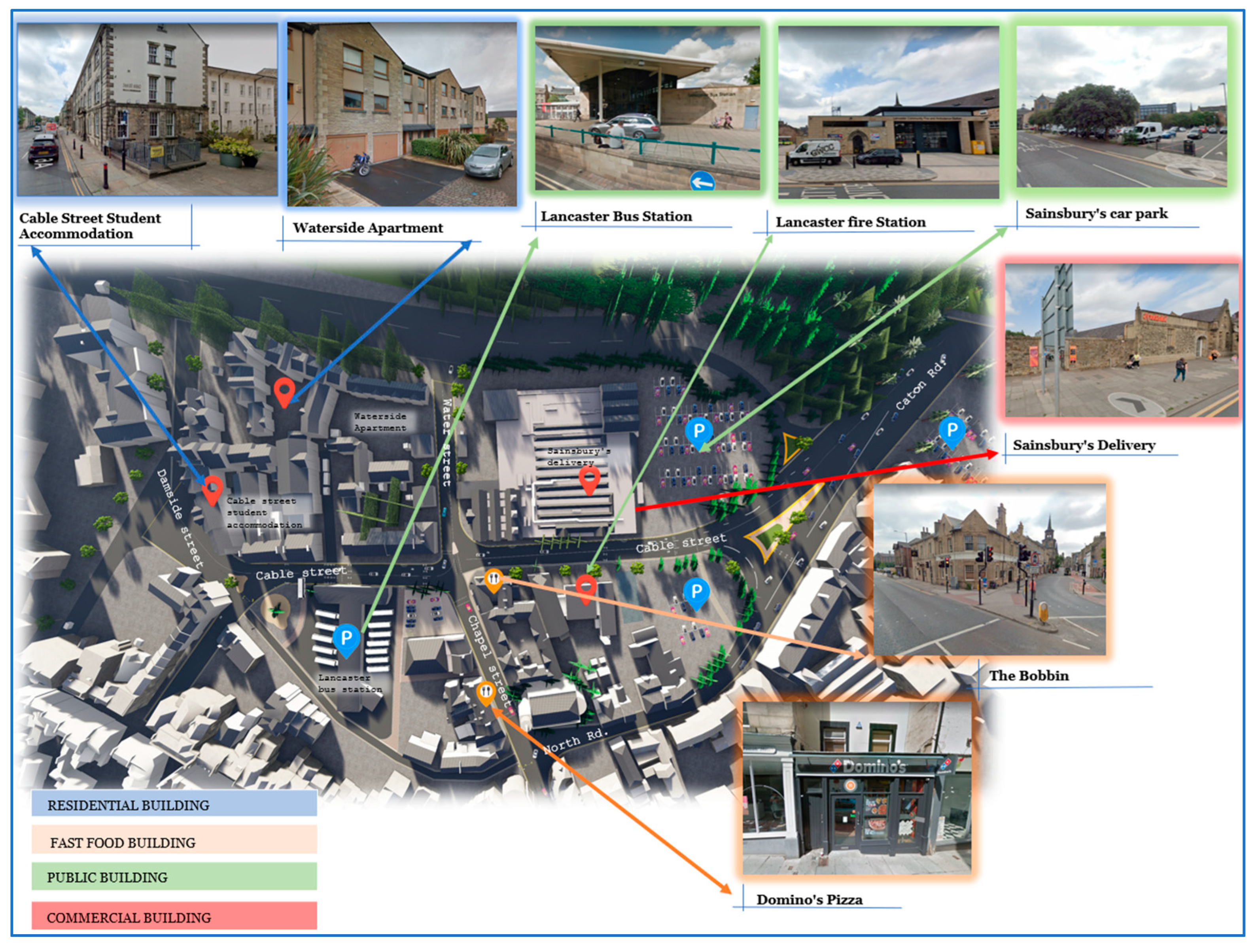
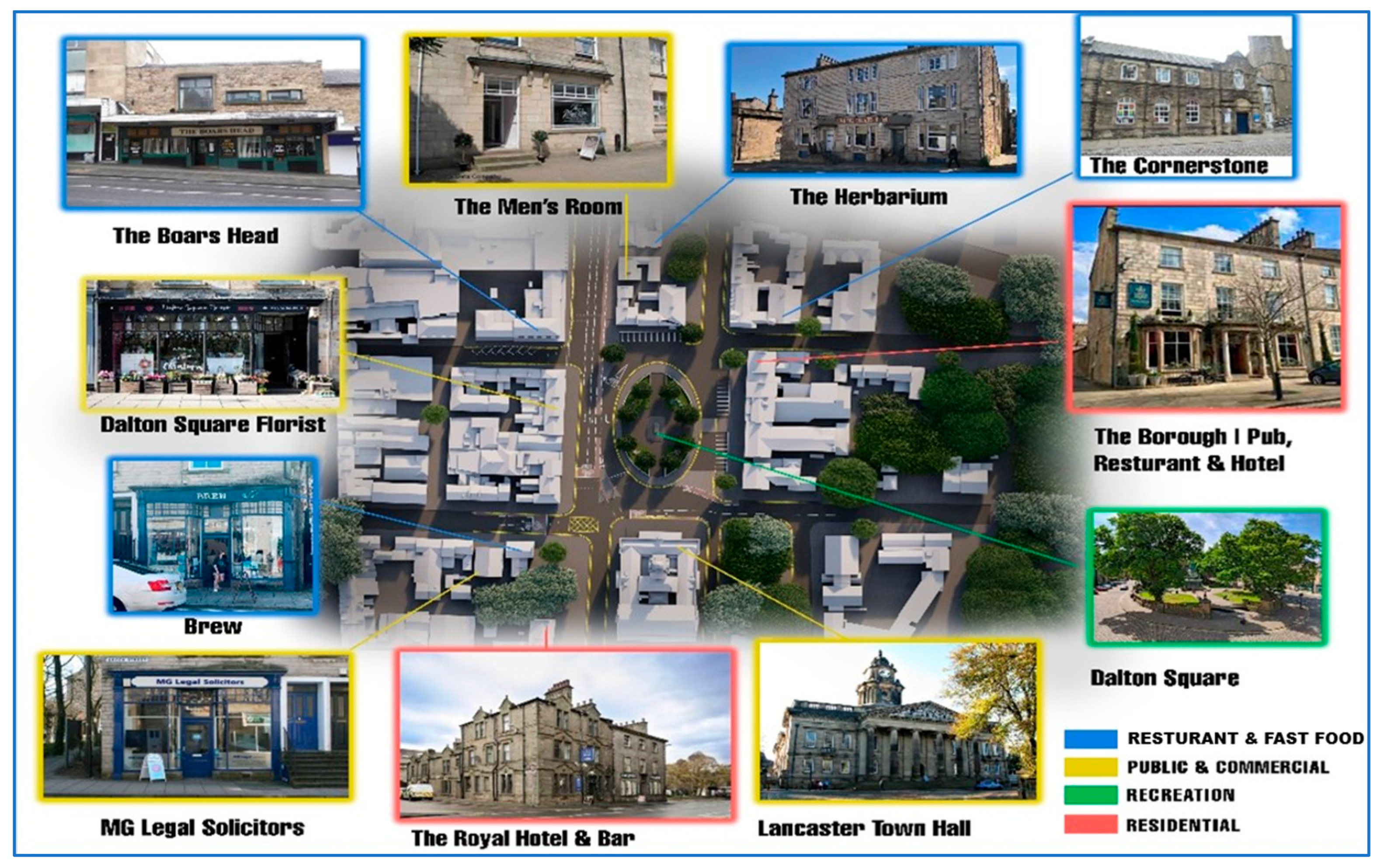
2.1. Site Description: Lancaster—Cable Street and Dalton Square

Lancaster is a small city in northwest England with a population of around 150,000 and a land area of 5700 km² [74,75]. Air pollution in Lancaster primarily stems from road transport, which accounts for ~45% of the overall pollution in the urban air [76]. Within Lancaster City Centre, Cable Street is a hub for commuting, shopping, and leisure, experiencing heavy traffic during business hours. Bordered by a major supermarket, Lancaster Bus Station, and the river Lune, it serves as a crucial transportation corridor connecting the city centre, railway station, and suburbs (Figure 1). The bus station, a key transportation hub, attracts around 7000 daily passengers [77]. Approximately 20,000 vehicles navigate Cable Street daily [78], causing congestion and high vehicular emissions. With around 3000 pedestrians using the route, this poses significant implications for air pollution exposure and public health [79]. Dalton Square is a leisure area with various features such as trees, benches, and a statue of Queen Victoria. It is surrounded by different buildings and streets, including the Town Hall, office and community buildings, and retail and leisure buildings (Figure 2). Thurnham Street is a major route that connects the square with the city centre. It receives ~15,000 vehicles and 2000 pedestrians daily [77], with a very small proportion of the population using the square (Dalton Square) for relaxation. However, this changes with the time of the year, as is evident from the annual Lancaster on Ice event reported to attract ~35,000 skaters and 90,000 visitors every December, increasing traffic flow and potentially the concentrations of air pollution in Lancaster [80]. Therefore, it is important to establish the spatial and temporal variability of pollutant levels and the dynamics of population flow in the area during different seasons and times of day.

2.2. Air Quality Monitoring

This study uses hourly average NO₂ and PM₁₀ concentrations from the monitoring station co-located with the Central Bus Station on Cable Street and on Thurnham Street’s side of Dalton Square from January 2015 to January 2019 (www.ukairquality.net (accessed on 16 June 2020)). Cable Street and Dalton Square exhibit elevated NO₂ levels, often surpassing UK objectives, and particularly high PM₁₀ levels compared to other pollutants. To understand the different patterns and rhythms of air pollution within the study locations across different timescales, 5-year average hourly NO₂ and PM₁₀ concentrations were calculated for Cable Street for each day of the week for winter, summer, university term time, and non-university term times, and then compared to NO₂ concentrations at Dalton Square for the pre-defined periods.

2.3. Population Flow

To capture the flow of daily traffic and pedestrian rhythms in the study areas, we employed common empirical observation tools such as counting, mapping, sketches, field notes, and videography, often used in public-life studies [64,81,82,83,84]. On Cable Street, traffic and pedestrian flows were recorded for 5 min during every hour for each flow, starting at 6 am and ending at 10 pm, using a manual counter for sixteen days over 2 weeks, on consecutive Mondays, Thursdays, Saturdays, and Sundays during winter (23 November–5 January) and summer (16 August–30 August) of 2019 and 2021, respectively, to link traffic movement (vehicular and pedestrian) with air pollution in the street and at the bus station. The recorder was placed at different locations along the street during the defined observation periods. To calculate the hourly traffic flow, we multiplied the number of vehicles and pedestrians observed in 5 min by 12 (since there are 12 5 min intervals in an hour). For example, if 50 vehicles and 20 pedestrians were counted in 5 min, the estimated hourly flow would be 600 vehicles and 240 pedestrians. In addition to the empirical data, information on cumulative population travel and activity patterns extracted from Stagecoach (local company) bus timetables for the 2019/2020 and 2021/2022 transport years were used. The data were available at different temporal scales, including weekday, weekend, university term time, and non-university term time in summer (from the easter holiday to the end of the academic year in July) and winter transport seasons (between October and March). Diurnal plots were used to analyse hourly bus and pedestrian activity and offer insights into usage patterns at the bus station and Cable Street across various time scales. At Dalton Square, a CAT S60 Thermal Imaging device captured daily pedestrian and traffic flow for 8 days over 2 weeks (weekdays and weekends) during a single winter term (6 February–20 January), summer term (9–22 May), and summer vacation (15–22 August) in 2022. Traffic count data from the Lancaster on Ice event during the winter vacation of 2019 (16 December–30 December) were considered, with daily ice rink session counts provided by the organizers. Pedestrian and vehicle flow around the square obtained from video footage and the traffic recorders on Cable Street were coded to map flows and space rhythms and represented by unique colours, i.e., vehicular traffic (blue) and people (e.g., walking, cycling and stationary activities along the streets (black), as well as passengers at the bus station (red)).

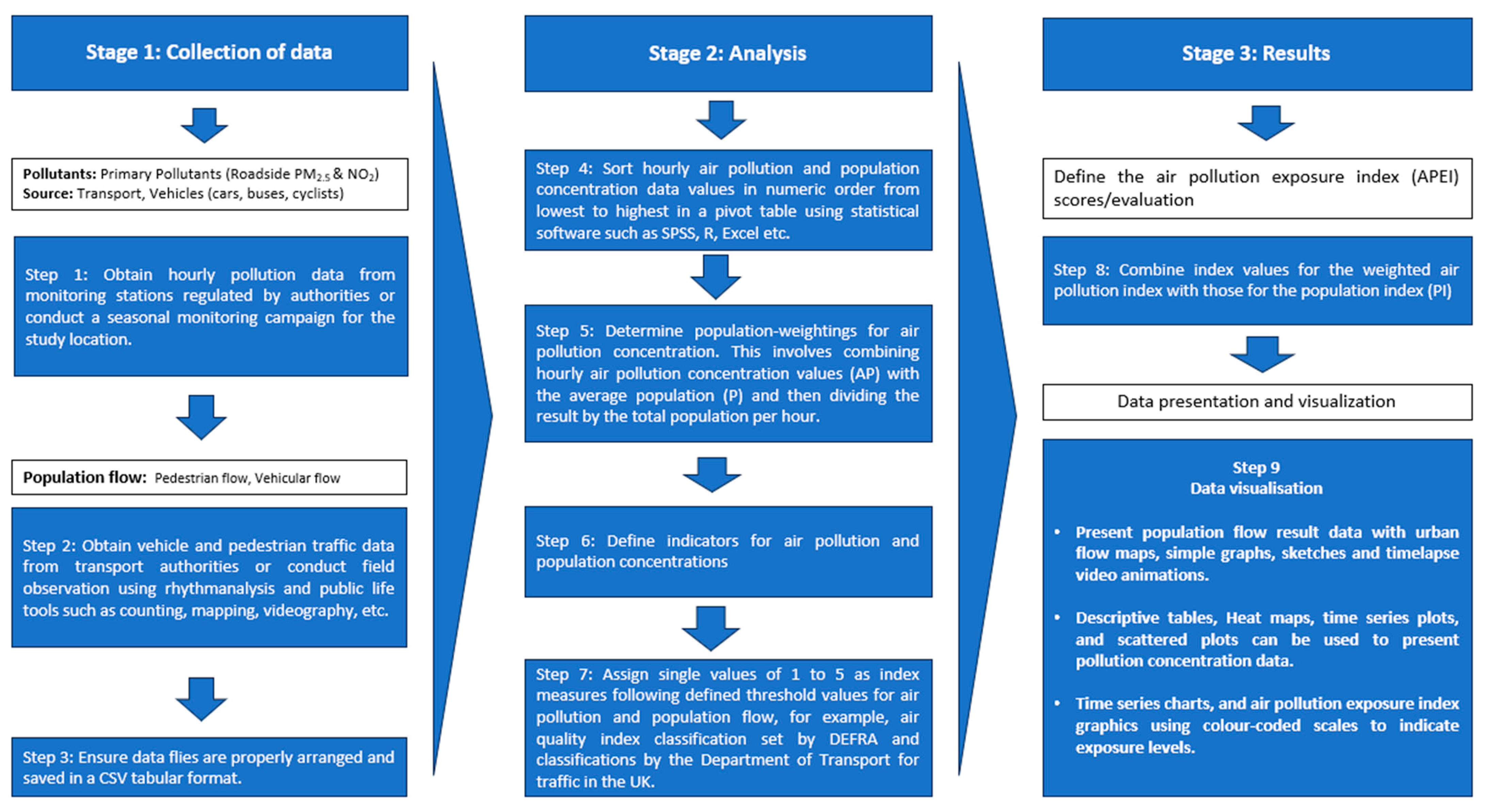
2.4. Air Quality Exposure Index

2.4.1. Setting out the Metric’s Stages and Parameters

The main steps in this phase involve sorting hourly air pollution (AP) and population concentration values (P), weighting air pollution exposure, assigning single values of 1 to 5 as index measures following the threshold values established in this study for air pollution and population, and finally, combining the index values for weighted air pollution exposure (WAPEI) with those for population (PI) to define the air pollution exposure index (APEI) scores. The APEI in this study uses numerical values used to describe different levels of air pollution exposure risk, with higher values indicating a greater likelihood of exposure. The index measure for WAPE levels (µg/m³) aligned with the hourly AQI and threshold values set by DEFRA [65] and the standards proposed in this study for assessing levels of population flow, i.e., low to high traffic and pedestrian flow on urban roads. Traffic and pedestrian flows refer to the rate at which vehicles and people pass a given point on the road and their values are given in vehicles or people per hour. Where specific hourly thresholds for air quality are not provided (for example, the WHO and DEFRA do not offer hourly thresholds for PM₁₀), daily mean AQ thresholds may be used. In cases where traffic and pedestrian flow standards are not defined, those suggested in this study can serve as a reference. However, we acknowledge the existence of alternative guidelines and procedures, which vary by location, context, and other factors, and are subject to change over time. As a result, our guidelines are not intended as a set of uniform standards for everyone to adhere to, nor are they intended to replace successful existing practices. Instead, we attempt to address common or specific issues regarding the classification and linking of population dynamics and air pollution data for busy urban areas. The parameters for air quality and traffic flow standards set out in this study are described below.

2.4.2. Traffic and Pedestrian Parameters

To set out traffic parameters for this study, it is important to note that the DfT does not provide specific threshold or classification values for average hourly traffic flow, and the definitions which describe these are not rigid. The DfT, as with most transport regulatory agencies, classifies traffic based on AADF (annual average daily traffic flow) [85,86,87,88,89], which represents the total volume of vehicle traffic on a motorway or road for a year, divided by 365 days. Specifically, vehicle traffic flows are classified according to road capacity, such as motorways (M roads), A, B and C roads, and unclassified roads. More information on the UK classification for and trends of vehicle flow by road is available at https://www.gov.uk/government/statistical-data-sets/road-traffic-statistics-tra#annual-daily-traffic-flow-and-distribution-tra03 (accessed on 15 May 2024).

• Motorways are the highest class of roads and are designed for fast-moving long-distance traffic. These roads handle very high traffic volumes of up to 100,000 vehicles per day or even more on the busiest sections.
• A roads are major urban routes that can be either primary or non-primary. Primary A roads can carry high traffic volumes of up to 50,000 vehicles per day, while non-primary A roads have less traffic than primary A roads and typically handle traffic of up to 20,000 vehicles per day.
• B roads are less significant than A roads and primarily serve to connect smaller towns and local destinations. These roads generally carry lower traffic volumes, usually up to 10,000 vehicles per day.
• C roads are important but smaller routes maintained by local authorities and often serve smaller towns and residential areas. These roads handle even smaller traffic volumes, typically under 5000 vehicles per day.
• Unclassified roads are minor roads intended for local traffic within towns and villages, including residential streets, rural roads and other minor roads. These roads usually have a very low traffic volumes, typically no more than 1000 vehicles per day.

Based on the above classification, the two study locations in central Lancaster, Cable Street and Thurnham Road, fall in the A roads category, as they receive approximately 20,000 vehicles per day [78].

Unlike vehicle traffic, there is no standardised categorisation for pedestrian traffic volumes on the different types of roads in the UK, and ground-truthing long-term data on pedestrian activity trends are unavailable. However, TfL’s survey of pedestrian activity (footfall, or pedestrian populations) in central London provides a comprehensive insight into hourly pedestrian activity trends across several London locations (which covers all road types [90]. Data suggest that the average pedestrian flows across central London typically do not exceed 900 pedestrians per hour [91]. While these data may not be representative of Lancaster’s pedestrian volume, they nonetheless offer a potentially useful benchmark for defining pedestrian populations in busy urban areas.

To define baseline hourly vehicle and pedestrian traffic thresholds for this study, we first converted the maximum AADF threshold value for A roads to average hourly flows and then subdivided it into five quantiles before assigning index values. To work out the conversion, the threshold value for AADF was simply divided by the total number of hours (T) during which traffic count was conducted to determine the annual average hourly traffic flow (AAHF), as seen in Equation (1):

$$\mathrm{A}\mathrm{A}\mathrm{H}\mathrm{F}=\frac{\mathrm{A}\mathrm{A}\mathrm{D}\mathrm{F}}{\mathrm{T}}$$

(1)

where AAHF is the annual average traffic flow per hour, AADF is the annual average daily traffic flow, and T is time in hours.

Subsequently, we divided the derived AAHF value into five quintiles, with the first quintile representing the lowest 1/5 of the values from 1 to 20% of the range, the second quintile representing values from 20 to 40%, the third quintile including 40 to 60%, the fourth quintile including 60 to 80%, and the fifth quintile representing the highest 1/5 of values from 80 to 100%. This helps to rank vehicles along the streets into potentially higher and lower concentrations. To rank them, single index values of 1 to 5 were assigned to each quintile range, with 1 assigned to lower values in the 1 to 20% quintile range, 2 assigned to values ranging between 20 and 40%, 3 to values between 40 and 60%, 4 assigned to values between 60 and 80% and 5 assigned to the highest values between 80 and 100%.

As with vehicle traffic, the maximum average hourly pedestrian flow value from TfL’s report was adopted as a proxy for the maximum hourly pedestrian population in busy urban areas, and then divided into five quintiles before being assigned index values similar to those used to determine the magnitude of the vehicle traffic flows. This was achieved by assigning single index values of 1 to 5 from lower to higher quintiles, with values below 180 assigned a value of 1 (very low), those ranging from 181 to 360 a value of 2 (low), values ranging from 361 to 540 a value of 3 (moderate), values ranging 541 to 720 a value of 4 (high), and those above 721 a value of 5 (very high). A summary of the population index and threshold values of traffic and pedestrian flows can be seen in

Table 1. Defined population index (traffic and pedestrian) and threshold values.

Population Index	1	2	3	4	5
Category	Very Low	Low	Moderate	High	Very High
Pedestrians per hour	0–180	181–360	361–540	541–720	721 or more
Vehicles per hour	0–417	418–834	835–1251	1252–1668	1669 or more
Percentile	1–20%	20–40%	40–60%	60–80%	80–100% or more

. Note that this benchmark is originally intended for defining population flow on A roads but can be used for other roads and in different locations to allow for better standardisation and validation of their suitability in various urban contexts.

2.4.3. Air Quality Parameter

We used the air quality index system set by DEFRA to determine low–high air pollution levels [92]. In particular, the AQI for NO₂ and PM₁₀ was refined to suit the levels and categorisation used for population dynamics in this study. Currently, the DEFRA-defined AQ index numbers rank between 1 and 10, with 1 to 3 representing varying degrees of low pollution concentrations, 4 to 6 representing varying moderate pollution concentrations, 7 to 9 representing various degrees of high concentrations, and 10 representing very high pollution concentrations. In this study, DEFRA’s index metric was regrouped into 5 categories, with category 1 indicating very low concentrations and aligning with a DEFRA pollution threshold value of 1, category 2 representing low pollution concentrations and DEFRA’s threshold values of 2 to 3, category 3 representing moderate concentrations and DEFRA’s pollution values from 4 to 6, category 4 representing high pollution concentrations and DEFRA’s pollution concentration threshold from 7 to 9, and category 5 representing high concentrations and pollution threshold values assigned an index number of 10 by DEFRA. The NO₂ and PM₁₀ threshold values set by DEFRA and those refined in this study are summarised in

Table 2. Daily air quality index and pollutant threshold values set by DEFRA.

Index	1	2	3	4	5	6	7	8	9	10
Band/Category	Low	Low	Low	Moderate	Moderate	Moderate	High	High	High	Very High
NO2 (µg/m3)	0–67	68–134	135–200	201–267	268–334	335–400	401–467	468–534	535–600	601 or more
PM10 (µg/m3)	0–16	17–33	34–50	51–58	59–66	67–75	76–83	84–91	92–100	101 or more

Note: available NO₂ threshold values are based on hourly mean concentration, while PM₁₀ particles are based on 24 h mean concentration.

and

Table 3. Air quality index and threshold values adapted from DEFRA’s AQI.

Air Quality Index (AQI)	1	2	3	4	5
Category	Very Low	Low	Moderate	High	Very High
NO2 (µg/m3)	0–67	68–200	201–400	401–600	601 or more
PM10 (µg/m3)	0–16	17–50	51–75	76–100	100 or more

.

2.4.4. Air Pollution Exposure Index Framework

We first sorted the NO₂ and PM₁₀ hourly values, a surrogate for pollution, and those of pedestrian and vehicle traffic, a surrogate for the population, in numeric order from lowest to highest in an Excel Pivot Table for a pre-defined study period. After sorting, we weighed air pollution exposure to NO₂ and PM₁₀ by multiplying their hourly mean pollution concentration values (AP) with average pedestrian flow values (P), and then divided the result by the total pedestrians per hour. This helped provide insight into the levels of pollution people are likely to be exposed to during the day.

$$\mathrm{W}\mathrm{A}\mathrm{P}\mathrm{E} \mathrm{t}\mathrm{o} {\mathrm{P}\mathrm{M}}_{10} \mathrm{o}\mathrm{r} {\mathrm{N}\mathrm{O}}_2=\frac{\sum {\mathrm{A}\mathrm{P}}_i\times {\mathrm{P}}_i}{\sum {\mathrm{P}}_i}$$

(2)

where $i=1,2,3,\dots ,n$, P_i is the average hourly pedestrian count, and AP_i is the hourly mean pollution concentration.

Following this, the hourly weighted air pollution exposure and population values (as in pedestrian flows) were assigned index numbers of 1–5, referencing the ranges in the AQI system and population index benchmarks presented in Table 1 and Table 3, respectively. The WAPE values for PM₁₀ and NO₂ were aligned with our refined air quality index guidelines because the weighted concentration values were given in micrograms per cubic metre (µg/m³). An index number of 1 was assigned to weighted concentrations matching very low categories. For example, all weighted NO₂ concentration values ranging between 0 and 67 µg/m³ were assigned a value of 1 (very low). This process was repeated for index numbers 2, 3, 4, and 5 across all the variables considered in this study. That is, a very high index value (5) would mean there is a very high population concentration, while a very low index value means a low population presence (Table 1).

Next, the index values assigned to hourly pedestrian flows (Table 1) were multiplied by those assigned to weighted NO₂ and PM₁₀ concentration, to derive the air pollution exposure index measures (APEI). APEI values were categorized on a scale from 1 to 25, i.e., the lowest to highest value of our APEI classification (

Table 4. Interpretation of the air pollution exposure index.

Air Pollution Exposure Index and Risk		Description
1–5	Very Low Exposure	Combination of any of the following: Low pollution and very low population; very low pollution and very low population; low pollution and low population; very low pollution and low population; very high pollution and very low population; very low pollution and high pollution; moderate pollution and very low population; very low pollution and moderate population.
6–10	Low Exposure	Combination of any of the following: low pollution and moderate population; moderate pollution and low population; high pollution and low population; low pollution and high population; very high pollution and low population; low pollution and very high population; moderate pollution and moderate population.
11–15	Moderate	Combination of any of the following: moderate pollution and high population; high pollution and moderate population; moderate pollution and very high population; very high pollution and moderate population.
16–20	High Exposure Risk	Combination of any of the following: high pollution and high population; high pollution and very high population.
21–25	Very High Exposure Risk	Combination of very high pollution and very high population.

). For example, if the index value for hourly levels of pedestrian flow (population) is 2 and that of weighted NO₂ is 5, the APEI value will be 10, and if the index value for hourly weighted PM₁₀ level is 5 and the pedestrian flow index is 5, the APEI value will be 25. APEI values in the range of 1–5 represent a very low risk of exposure, 6–10 indicate a low risk of exposure, 11–15 signify a moderate risk of exposure, 16–20 represent high risk of exposure, and 21–25 indicate a very high risk of exposure (Table 4). This indicates that locations and times with high population densities and air pollution levels pose the highest risk (e.g., APEIs from 21 to 25) compared to those with low population densities and pollutant concentrations (e.g., APEIs from 1 to 5). The APEI was used to characterize air pollution exposure during the days of various seasons. This involved analysing the frequency of occurrences within each index range (

Table 5. The frequency of occurrence of air pollution exposure categories on Cable Street during the day in different seasons.

Exposure Risk Categories	Air Pollution Exposure Index (APEI)	Frequency of Occurrences During the Day (in %)
		Weekday Summer Term		Weekday Winter Term		Sunday Winter Term		Sunday Summer Term		Weekday Summer Vacation		Sunday Summer Vacation		Weekday Winter Vacation		Sunday Winter Vacation
		NO2	PM10	NO2	PM10	NO2	PM10	NO2	PM10	NO2	PM10	NO2	PM10	NO2	PM10	NO2	PM10
Very Low Exposure	1–5	100	80.4	100	91.7	100	100	100	100	100	58.3	100	95.8	100	91.7	79.2	75
Low Exposure	6–10	00	16.6	00	8.3	00	00	00	00	00	41.6	00	4.2	00	8.3	20.8	25
Moderate Exposure	11–15	00	00	00	00	00	00	00	00	00	00	00	00	00	00	00	00
High Exposure	16–20	00	00	00	00	00	00	00	00	00	00	00	00	00	00	00	00
Very High Exposure	21–25	00	00	00	00	00	00	00	00	00	00	00	00	00	00	00	00

,

Table 6. The frequency of occurrence of population categories on Cable Street during the day in different seasons.

Population Categories	Index Score	Pedestrian Population (Pedestrians per Hour)	Frequency of Occurrences During the Day (in %)
			Weekday Summer Term	Weekday Winter Term	Sunday Winter Term	Sunday Summer Term	Weekday Summer Vacation	Sunday Summer Vacation	Weekday Winter Vacation	Sunday Winter Vacation
Very Low Population	1	0–180	54.2	58.3	87.5	79.2	37.5	68.5	50.0	45.8
Low Population	2	181–360	43	39.2	12.5	20.8	42.3	28	38.2	29.2
Moderate Population	3	361–540	3	2.5	00	00	16.0	3.5	8.3	20.8
High Population	4	541–720	00	00	00	00	4.2	00	3.5	2.2
Very High Population	5	721 and more	00	00	00	00	00	00	00	2.0

and

Table 7. The frequency of occurrence of air quality categories on Cable Street during the day in different seasons.

Air Quality Categories	Index Score	NO2 Conc. Value µg/m3	PM10 Conc. Value µg/m3	Frequency of Occurrences During the Day (in %)
				Weekday Summer Term		Weekday Winter Term		Sunday Winter Term		Sunday Summer Term		Weekday Summer Vacation		Sunday Summer Vacation		Weekday Winter Vacation		Sunday Winter Vacation
				NO2	PM10	NO2	PM10	NO2	PM10	NO2	PM10	NO2	PM10	NO2	PM10	NO2	PM10	NO2	PM10
Very Low Pollution	1	0–67	0–16	100	8.4	100	27.5	100	14.4	88.3	14	100	23.2	100	65.7	100	24.2	54.2	45.7
Low Pollution	2	68–134	17–50	00	91.6	00	72.5	00	85.5	16.7	96	00	76.8	00	34.3	00	75.8	45.8	54.3
Moderate Pollution	3	201–400	51–75	00	00	00	00	00	00	00	00	00	00	00	00	00	00	00	00
High Pollution	4	401–600	76–100	00	00	00	00	00	00	00	00	00	00	00	00	00	00	00	00
Very High Pollution	5	> 601	> 101	00	00	00	00	00	00	00	00	00	00	00	00	00	00	00	00

). The results were then combined and represented on a single diurnal plot to better understand the hourly or seasonal changes in rhythms and patterns of exposure. These methods were then applied to Dalton Square and the evolving results were compared to those of Cable Street to understand the different patterns and rhythms of air pollution exposure over the range of interest. A summary of our methodological framework is presented in Figure 3.

3. Results

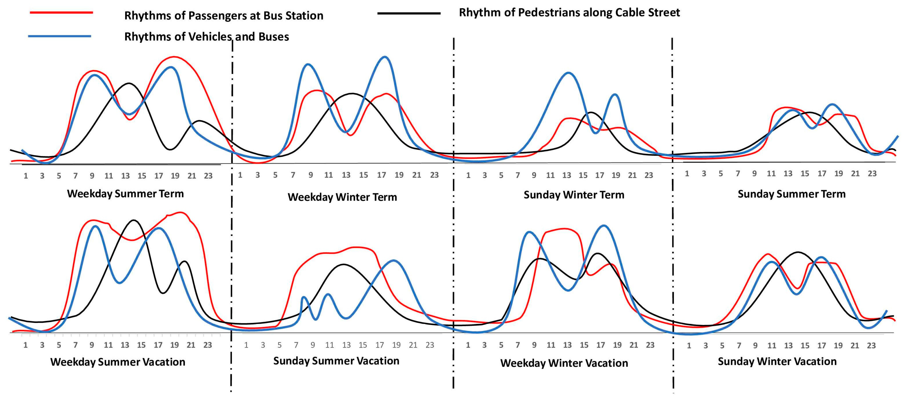
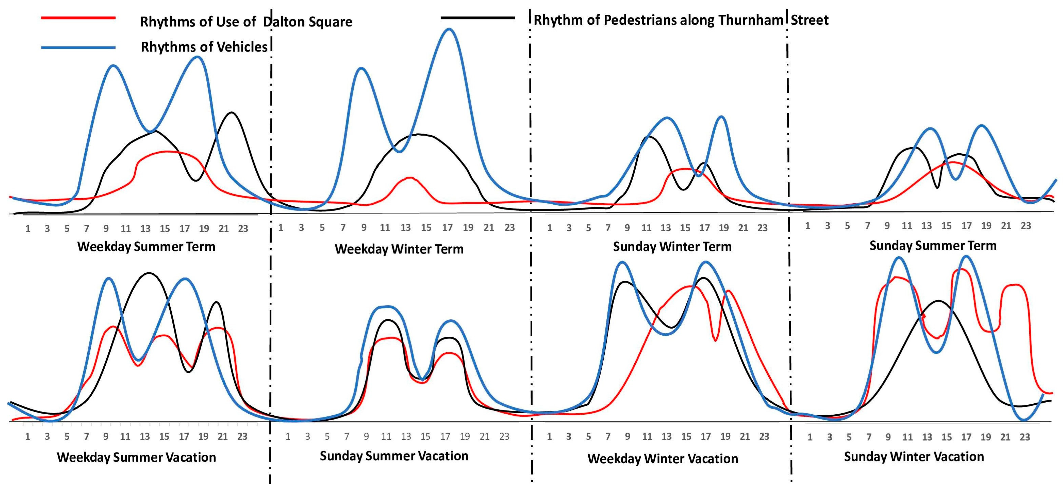
3.1. Rhythm of the Public Space

3.1.1. Cable Street

Figure 4 shows the seasonal rhythm of people and vehicle flows along Cable Street and the bus station following Lancaster University’s and the bus operator’s timetable’s temporal classifications. The data suggest public use of Cable Street during a typical weekday in the summer term, which spans from the Easter holiday to the end of the academic year in July [93,94], starts at 04:30 when the bus station opens, and ends at 00:00 when it closes during term time. Traffic peaks occur from 08:00 to 11:00 and 15:00 to 19:00, with a significant morning rush at 08:00 due to the opening of businesses, offices, and educational establishments in Lancaster. Passenger and bus traffic at the station also peaks at this time. After 10:00, commuting declines, but pedestrian traffic increases, peaking at 13:00. Evening activity heightens again until around 18:00, with a notable peak at 21:00 when retail outlet, restaurant, and bar closures commence.

In the winter term (which is from October to December (Michaelmas term) and January to March (Lent term) at Lancaster University [94]), daily commuting starts later at 06:00, with higher vehicle numbers but lower passenger and pedestrian presence due to weather conditions or reduced bus routes [95]. Morning traffic peaks similarly at 08:00, and pedestrian traffic rises at 13:00. The 10–13:00 off-peak period observed in summer is also seen in winter. Pedestrians along Cable Street increase during these hours, peaking at 13:00, contrasting with summer when peaks occur in the morning and late evening. Evening congestion is less severe compared to summer, and transport activities decline after 19:00, with the last buses departing at 00:00.

Sundays during both terms see quieter streets, with bus services starting later than on weekdays. Winter Sundays have more vehicle traffic, but fewer pedestrians compared to summer. Passenger presence at the station begins at 8:00 in both seasons, with pedestrian activity on Cable Street starting at 8:00 in summer (primarily cyclists and walkers) and 11:00 in winter when businesses in the city centre open on Sundays. Winter transport activity at the station surpasses that of summer, with a 400% increase in buses and vehicles and a 150% rise in passengers. The peak in winter-term passengers and bus activity is at 13:00, which coincides with intense retail and leisure activity in the city centre, while that of 19:00 during the summer term contrasts with this. Although relatively lower than on weekdays, pedestrian peaks occur in the late evening on Sundays despite the early closure of the bus station and most restaurants and pubs.

During the summer vacation (mid-July to mid-September), activity resembles winter weekdays, with higher transport and pedestrian presence along the street due to increased outdoor activities following favourable weather conditions, leisure time, and holiday travel. The bus station and Cable Street are busiest with higher numbers of vehicles and pedestrians, almost twice those of the summer term. This is attributed to expanded intra-urban transit routes in summer, extending to challenging winter-accessible holiday locations, such as the North Lake District (Kendal, Ambleside, Keswick), served by the daily 555 and 755 services introduced during this period [95,96]. Vehicle and pedestrian numbers peak around midday (around 12–13:00) and early evening (~20:00) compared to the summer term, when an increase was observed into the late night.

As expected, the slow rhythm on the street on typical Sundays is observed during Sundays in the summer vacation, despite more people using the street and bus station than during term time. Passengers are observed to increase at the station earlier than usual for weekend mornings, while pedestrian traffic matches that of Sundays during term time. Vehicle and bus flow begins at 06:00, declining after 8:00, with no bus arrivals or departures until ~09:00 when traffic resumes, and minimal peaks at 08:00 and 11:00 are observed, in contrast to summer term. Evening bus and car traffic on the street and in the station, like in the summer term, peaks at around 19:00 and is highest at this time compared to weekends during the summer term.

In contrast, winter vacation (mid-December to early January) is characterised by increased bus and pedestrian presence due to holiday events in Lancaster, driven by an influx of visitors for Christmas and the annual Lancaster on Ice event during this time of the year. Vehicle and bus flow on Cable Street begins at 06:00 on both weekdays and weekends, with passenger activity starting later on weekdays and peaking around 8:00 on weekdays and 11:00 on weekends. A noticeable divergence occurs between weekday and weekend activities from 10:00 to 13:00, particularly with the high passenger numbers at the bus station during typical off-peak hours. Transport activities at the station were relatively higher on weekdays than on weekends, peaking at 17:00 on both weekdays and weekends. Consistent with a typical winter vacation weekday/weekend, activity on the street and at the bus station declines at 22:00.

3.1.2. Dalton Square vs. Cable Street

Figure 5 indicates that public use of Dalton Square on a typical summer term weekday begins around 07:00, with vehicle and transport activity on Thurnham Street starting as early as 05:30. Traffic peaks correlate with high activity on Cable Street during the morning and evening rush hours. Pedestrian numbers are lower in the morning, with the square busiest from 13:00 to 15:00. Thurnham Street and the surrounding areas experience higher pedestrian traffic than Cable Street, being closer to residential and retail areas. Traffic congestion on Cable Street extends to Thurnham Street during peak hours, emphasizing that Dalton Square’s rhythm is largely interlinked with the rhythms of businesses, educational establishments, and offices in Lancaster and around the city centre.

In the winter term, commuting starts at 06:00, with higher vehicle activity on Thurnham Street in the morning and evening compared to summer-term weekdays. Peaks in vehicles and pedestrians align with high activity on Cable Street. However, minimal pedestrian presence is recorded at the square during these hours, with the highest levels at 13:00 considerably lower than in summer. The afternoon peak is similar to that in summer, with less time spent at the square, even when pedestrian traffic on Thurnham Street is maximal. On average, the square is busier during summer weekdays than in winter, suggesting fewer engagements during the latter, possibly due to Lancaster’s weather or reduced outdoor activities.

During summer weekends, pedestrian and vehicular traffic peaks between 6:30 and 11:00, with evening peaks aligning somewhat with Cable Street on both winter- and summer-term weekends. Morning pedestrian activity in the square increases, significantly peaking at 11:00. While morning sidewalk usage is 198% greater than on Cable Street, vehicle traffic on Thurnham Street is 14% lower. This continues into late afternoon (~15:00), contrasting with weekdays. Evening vehicle concentration peaks at 16:00, and is 6% lower than on Cable Street in winter or summer, with pedestrians 3% lower. Sundays see higher square activity, with a busy atmosphere due to more leisure shopping or socializing, especially during summer. Generally, Dalton Square is busier on summer weekends than winter, while Thurnham Street has lower vehicular activity compared to Cable Street in these seasons.

On summer vacation weekdays, Dalton Square is significantly busier than in term time, with activity peaks at 10:00, 14:00, and 20:00. More people spend time in the square, likely influenced by Lancaster’s summer conditions, extending into late evening (~20–21:00). Thurnham Street sees increased vehicular and pedestrian traffic, aligning with Cable Street’s peak times (08:00 for vehicles, 16:00, and peaks at 13:00 and 20:00 for pedestrians). The afternoon (13:00) witnesses the highest pedestrian count, coinciding with peak shopping in the city centre. Despite higher vehicular traffic on Cable Street, Thurnham Street sees more pedestrians during summer vacation weekdays. This increased street activity is attributed to the increased level of outdoor activity in the city centre, including commuting activities resulting from the expansion of intra-urban transit routes during the summer.

However, during summer vacation weekends, both vehicle and pedestrian activities are fewer compared to term time. Morning usage is higher than in the evenings on Thurnham Street and Dalton Square, unlike weekdays. Pedestrian flow starts at 07:00 on the street and vehicles at 8:00 in the square, 30 min later than on Cable Street. Flow in the square peaks at 11:00, coinciding with increased traffic (pedestrian and vehicular) along the street and the pedestrian traffic peak on Cable Street. Vacation weekends show vehicle peaks in both the morning and slightly earlier in the evening (~17:00). Evening vehicle and pedestrian numbers are approximately 150% lower than on Cable Street, while Dalton Square is around 100% busier. Pedestrians numbers on the road and in the square are highest at this time compared to summer-term weekdays. Despite some differences between the two areas, the flow of people and vehicles around Dalton Square, Cable Street and the city centre aligns throughout most of the day.

During the winter vacation, changes are seen in the spatial and temporal use of Dalton Square due to the Christmas Market and Lancaster on Ice Event, attracting a considerable number of people and vehicles to the square and the city centre from early December to early January (Figure 4). The busiest times are the mid-afternoon (~15:00) and evening on weekdays (~19:00), and the morning, mid-afternoon, and evening on weekends (~11:00, ~16:00, ~21:00). Like Cable Street, Thurnham Street sees vehicles and pedestrians twice during the morning and evening on weekdays and mid-afternoon on weekends, with pedestrians peaking with vehicles, except for weekday evenings. However, the peak of activities in the Square is quite dissimilar.

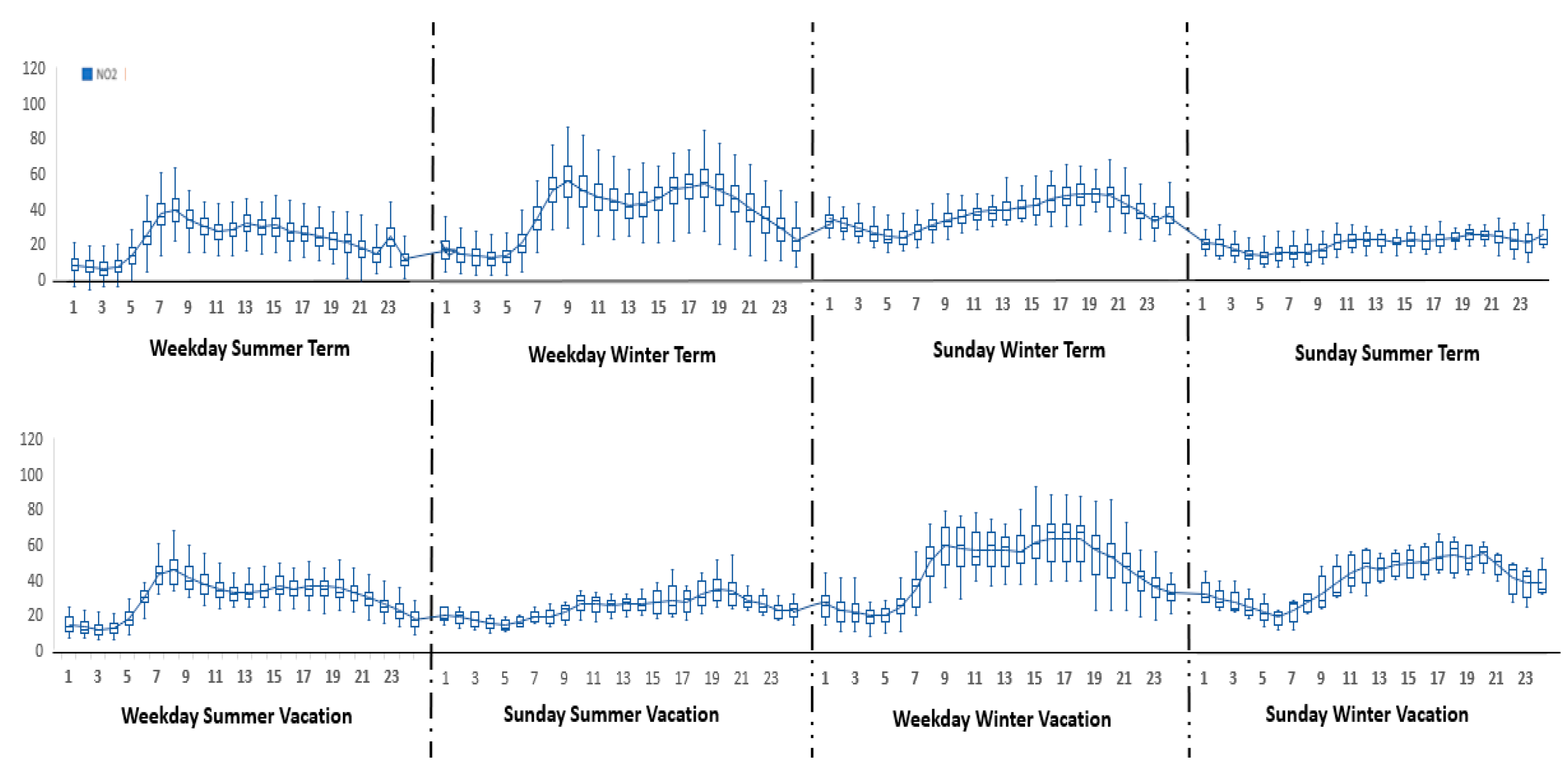
3.2. Rhythm of Pollution Concentration

3.2.1. Cable Street

The data show the seasonal hourly diurnal cycle of PM₁₀ and NO₂ on Cable Street during the different periods of the year described in the previous section (Figure 6). Pollution levels for most of the day and seasons correlate with transport rhythms in Lancaster, except for the early evening hours when contrast is observed.

On a typical weekday during the summer term, NO₂ and PM₁₀ levels on Cable Street begin increasing from 04:00 with the start of daily commuting, peaking at 08:00 during the morning rush and 17:00 as the evening rush commences. The maximum peak pollution concentrations occur during the evening rush hour (17:00), while the lowest levels are recorded at night (01:00). Similarly, PM₁₀ peaks at 18:00 and reaches its lowest at 01:00, coinciding with reduced street activity. During the winter term, NO₂ and PM₁₀ levels follow a similar summer morning pattern, but NO₂ peaks around 18:00 due to increased car traffic. Unlike summer, PM₁₀ does not decline until around 16:00. NO₂ declines after 18:00 as vehicular traffic decreases. The decline and the evening peak in NO₂ levels are consistent with vehicular flow and bus activities, while the pattern for PM₁₀ is different. However, the levels of NO₂ are relatively higher in winter than in summer due to increased car use and changes in meteorology.

Sundays show lower pollutant levels compared to weekdays, with higher concentrations in winter despite fewer vehicles, likely due to meteorological factors. In summer, NO₂ levels begin increasing 2 h later than on weekdays (~6–6:30), while PM₁₀ is the same as on weekdays, even when Sunday commuting patterns differ from weekdays. Unlike weekdays, increased concentration fluctuations occur later in the day, with NO₂ peaking from 11:00 to 13:00, and PM₁₀ showing peaks at 13:00 and 19:00. In winter, unlike in summer, both NO₂ and PM₁₀ increase from ~6 to 6:30. While fewer fluctuations occur in winter, NO_2, unlike in summer, increases until around 16:00, and PM₁₀ until 19:00. Peak NO₂ levels are observed at 15:00 and 20:00. In general, winter concentration peaks (PM₁₀ and NO₂) do not align with Cable Street’s vehicular rhythms during the summer term, despite higher vehicle numbers in winter.

During the summer vacation, despite higher vehicle numbers associated with increased outdoor and transport activities, pollution levels are generally lower on weekdays during summer vacation than term time. Akin to the summer term, NO₂ and PM₁₀ concentrations increase ~2 h earlier than the start of daily commuting on Cable Street, peaking at 8:00 and again at 17:00 before declining until the next day. NO₂ peaks during these times reflect the morning and evening rush at the station and in the street, while evening PM₁₀ differs. Similarly, pollution on Sundays during summer vacation follows a term-time pattern, with NO₂ and PM₁₀ levels rising with the bus station opening at 06:00 and peaking at 11:00 with the Sunday morning rush hour and at 17:00 during the evening transport rush hour along the street and within the station. However, both NO₂ and PM₁₀ pollution are higher in the summer term than during summer vacation. Surprisingly, NO₂ is 43% higher and PM₁₀ is 3% higher in the summer term, despite slightly more intra-urban transit routes and buses on Sundays during summer vacation.

Winter vacation sees increased pollution due to festive activities and higher levels of vehicle traffic, with weekday peaks at 09:00 and 18:00, and weekend peaks aligning with increased city centre activity, declining after 18:00. Compared to summertime, winter weekday morning NO₂ and PM₁₀ concentrations (Figure 5) increase from 05:00 and increase from 09:00 to 11:00 on weekends. Peaks at 09:00 and 18:00 on weekdays and 17:00 on weekends align with the city centre activity patterns described earlier. While NO₂ and PM₁₀ gradually increase from 05:00 to 12:00 on winter and summer vacation weekdays, weekends show a contrast, resembling winter term with increased levels from 08:00 to 20:00. Pollution levels are higher in the mornings and evenings on weekdays and throughout the day on weekends.

3.2.2. Dalton Square vs. Cable Street

The data suggest that morning NO₂ levels in Dalton Square during summer-term weekdays rise concurrently with those on Cable Street, peaking at 08:00 during the morning rush. NO_2′s decline from 08:00 to 13:00 on Cable Street is mirrored on Thurnham Street, attributed to reduced vehicle and transport activities in the gyratory system connecting the streets. NO₂ increases on Cable Street after 13:00 are also observed on Thurnham Street, with peaks occurring ~3 h later due to reduced traffic. Unlike Cable Street, NO₂ levels on Thurnham Street gradually decrease after 13:00 until a minimal peak at 23:00, even when vehicle traffic is observed to be lowest. This peak is likely from idling vehicles seen near the traffic light close to the air quality monitor on Thurnham Street.

The air pollution patterns on Thurnham Street and Cable Street during the winter term are relatively similar, though morning NO₂ levels are higher on Thurnham Street and evening NO₂ is higher on Cable Street (Figure 7). Morning (08:00) and evening (18:00) NO₂ peaks align with Cable Street’s pollution and vehicular traffic peaks, linked to the start and closure of business, educational, and office activities in Lancaster causing slower traffic flow on Thurnham Street. Pollution declines on Cable Street and Dalton Square from 10:00 to 13:00 are attributed to the vehicle off-peak period within the city centre.

On weekends in both the winter and summer seasons (Figure 7), NO₂ pollution varies between Cable Street and Thurnham Street. Thurnham Street exhibits higher NO₂ pollution during winter weekends despite more traffic emissions in the summer term. Pollution on Thurnham Street and Dalton Square increase simultaneously (~6–6:30) in both seasons until around 11:00, with a slight summer decline and constant winter levels, contrasting with Cable Street. Unlike Cable Street, Thurnham Street’s NO₂ levels increase again after 13:00 until 19:00 in winter, while summer weekdays show consistent levels until around 19:00 when both areas see declining pollution. NO₂ peaks are similar in summer but differ in winter between Cable Street and Thurnham Street, despite similar vehicle flow.

During summer vacation weekdays on Thurnham Street, NO₂ concentration rhythms resemble those in the summer term, though they are notably higher, akin to Cable Street. Morning NO₂ increases concurrently with that of Cable Street, with peaks aligning with Cable Street and city centre pollution and vehicle traffic highs. Unlike Cable Street, Thurnham Street records its highest pollution levels in the morning and the lowest in the evening. A contrast is seen on weekends during summer vacation on Thurnham Street. NO₂ levels are highest in the evening at around 19:00 and lowest in the morning from around 10:00 to 15:00. The morning peak coincides with the morning rush hour and NO₂ peak on Cable Street. The evening peak in NO₂, however, is delayed by ~2 h compared to Cable Street. Similar to Cable Street, NO₂ increases with morning traffic from ~06:00, maintaining a steady flow from ~10:00 to 15:00. In contrast to Cable Street, NO₂ levels continue to rise after this period. Thurnham Street’s hourly NO₂ concentrations are relatively higher than Cable Street’s during weekends, despite lower vehicular traffic.

Some similarities are seen in NO₂ levels on Thurnham Street and Cable Street during the winter vacation (Figure 7). As expected, pollution peaks during the winter holidays, exhibiting similar concentration rhythms at both locations on weekdays and weekends. NO₂ concentrations on Thurnham Street during winter weekday mornings begin simultaneously with those on Cable Street, but the peak times at 08:00 and ~15:00–18:00 differ from those on Cable Street. Similarly, weekend patterns are inconsistent with the pollution and traffic on Cable Street, with peaks at 11:00, 18:00, and 20:00. NO₂ levels on weekdays and weekends during winter vacation are marginally higher on Thurnham Street than on Cable Street. Overall, Cable Street and Dalton Square show a consistent pattern of pollution rhythm year-round, indicating traffic as the primary air pollution source. The levels of pollution and space occupation vary from season to season, with potential consequences for air pollution exposure and public health.

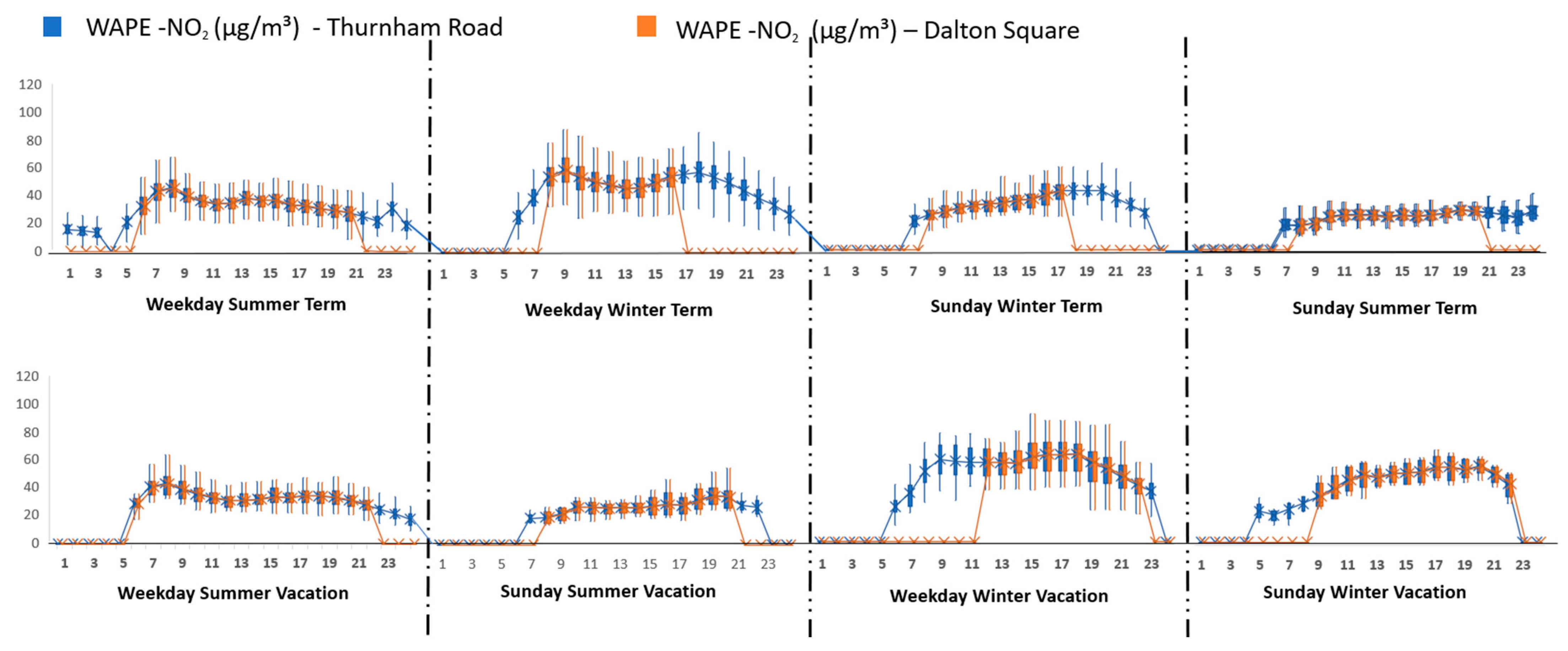
3.3. Weighted Air Pollution Exposure (WAPE)

Figure 8 and Figure 9 show the hourly weighted air pollution exposure (WAPE) to NO₂ and PM₁₀ on Cable Street and Dalton Square/Thurnham Road across different seasons. On Cable Street, the estimated weighted exposure levels to both NO₂ and PM₁₀ are generally consistent with the average diurnal concentrations of PM₁₀ and NO₂ described in Section 3.2.2 for most of the day. However, there is a significant difference in the late night to early morning hours, indicating a minimum concentration of pollution during this period, likely due to minimal pedestrian presence on the street during the quiet of the night. During these key periods, the weighted NO₂ concentrations range from 0 to 65 µg/m³ and 0 to 40 µg/m³ for PM₁₀, with concentrations not exceeding moderate levels based on our AQI system. This suggests that people using the street and bus station during these seasons are likely to experience higher pollution concentrations than others. Overall, the hourly WAPE to NO₂ and PM₁₀ is highest during weekdays in the summer and winter terms and lowest on Sundays during summer vacation.

At Dalton Square and on Thurnham Road, like Cable Street (Figure 8), WAPE NO₂ levels are consistent with the average daily pollution concentrations, except during the early morning and late evening hours at Dalton Square, across most seasons. The pattern of weighted NO₂ at Dalton Square is primarily influenced by public use of the square, with higher usage seen in the early mornings during the summer and later in the winter, except during the Lancaster on Ice Event, when the square is used into the late evening. Unlike on Cable Street, the hourly weighted NO₂ levels are highest for much of the day during weekdays in the winter term and weekdays during winter vacation on Thurnham Road and lowest on Sundays in the summer term and Sundays during summer vacation. Generally, the pattern of WAPE levels differs from that of Cable Street in almost all seasons, with the population at Dalton Square likely exposed to higher levels of NO₂ than that on Cable Street, ranging from 0 to 75 µg/m³. To address this issue, it is important to first understand the different patterns and rhythms of air pollution exposure with the usage of urban spaces during the study periods.

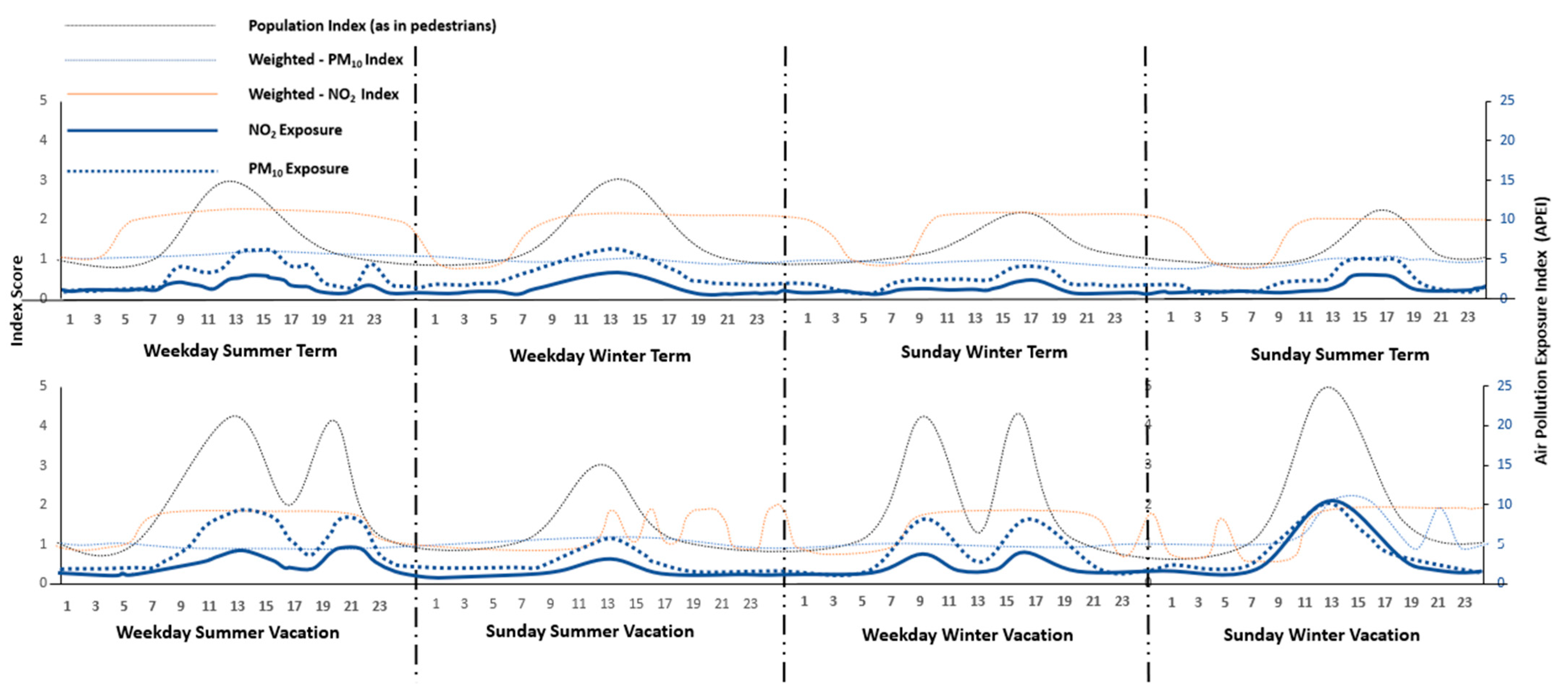
3.4. Population Exposure Rhythms

3.4.1. Cable Street

Table 5, Table 6 and Table 7 and Figure 10 show the frequency of occurrences and rhythms of exposure to air pollution on Cable Street across different seasons. During weekdays in the summer term, the risk of exposure to levels of NO₂ and PM₁₀ is very low for a major part of the day, particularly from around 01:00 to 07:00 and after 23:00. Both NO₂ and PM₁₀ exposure levels peak at 08:00, between 11:00 and 18:00, and at 22:00. The pollution concentration index is significantly low during these hours compared to other times of the day, with NO₂ indicating low pollution levels for a significant length of time during the day, and PM₁₀ even lower. NO₂ and PM₁₀ exposure risk is highest between 11:00 and 18:00, at which times Cable Street and the bus station are most used. The peak at 8:00 coincides with the opening hours of businesses, educational establishments, and offices in Lancaster, and the afternoon peak with rush hours associated with the lunch break, while the evening peak at 22:00 coincides with the closing hours of the bus station, as well as restaurants and pubs around the city centre.

Winter-term weekday NO₂ and PM₁₀ exposure risks remain significantly low for most of the day, as they are in the summer term (Figure 10). However, their levels and rhythms in winter and summer differ, while those for population flow and pollution are similar in both winter and summer. Unlike summer-term weekdays when NO₂ and PM₁₀ exposure peak minimally at ~22:00, no peak is observed at this time during the winter term. The highest exposure index values between 08:00 and 18:00 can be attributed to intense transport, commercial, and leisure activities during these hours. This is consistent with the times of the day when Cable Street and the bus station are most used during the day and when businesses, educational establishments, and offices in Lancaster and the city centre are open. Overall, the exposure risk on Cable Street is higher in the winter than in the summer.

On Sundays in the summer term, NO₂ and PM₁₀ exposure increase from 06:00, which is surprising given that the public use of the street and the bus station during the weekend only begins to be significant several hours after. The NO₂ and PM₁₀ exposure peaks between 14:00 and 20:00 align with the times typically busiest on Sundays. However, the levels of NO₂ and PM₁₀ exposure during Sundays in the winter term differ from those of the summer term, even though the rhythm of exposure as well as pollution and population concentrations are similar. As with the winter term, exposure to NO₂ and PM₁₀ generally increases with Sunday commuting, with maximum levels corresponding to the peak of Sunday business in Lancaster city centre. The minimum levels recorded in the early morning and late evening hours can be attributed to the reduced traffic experienced on the street during such hours. These results indicate a strong relationship between pollution and traffic levels on summer and winter days.

As expected, the levels of NO₂ and PM₁₀ pollution exposure are significantly higher during summer vacation weekdays, as shown in Figure 10 and Table 5. This is particularly true between the late morning to early afternoon hours and the late evening when the maximum and minimum peak NO₂ and PM₁₀ exposures are recorded. NO₂ exposure peaks during the late morning and evening hours are lower and indicate very low exposure risk, while PM₁₀ exposure peaks are higher and indicate low exposure risk. These peaks correspond with hours when pedestrian numbers are highest in the morning and evening hours. NO₂ and PM₁₀ concentrations are relatively constant with very low and low indexes throughout the day. The high index population values during summer vacation weekdays can be attributed to the increased outdoor and transport activities typically associated with vacation periods in Lancaster.

The levels of pollution exposure on weekends during summer vacation are generally lower than on weekdays. On the weekends, the risk of NO₂ and PM₁₀ exposure is very low for most of the day, except for mid-day hours (between 11:00 and 14:00), when the exposure peaks. This corresponds with times of intense vehicular and pedestrian traffic along the street. The pollution rhythms during summer vacation weekends differ from those at other times of the year. The highest index population value during noon can be attributed to the start of business on Sundays in and around the city centre. During these hours, the pollution concentration index is significantly low, and the population is moderate. The comparatively lowest pollution levels on weekends during summer vacation suggest low vehicle traffic, despite pedestrian presence on the street being higher than usual for a Sunday.

Weekdays are associated with very low exposure for most of the day, while weekends are associated with very low to moderate exposure. Both NO₂ and PM₁₀ exposure peak at 09:00 to 16:00 during weekdays, and around 13:00 on weekends. The weekday peaks correspond with intense commuting and engagement in the city centre. That of weekends corresponds with the times when vehicular traffic along the street increases significantly. During these times, the concentration levels of PM₁₀ and NO₂ pollution are low for a significant length of time on weekdays and weekends, with peak NO₂ concentrations recorded at 15:00 and 21:00 on weekends and none on weekdays. However, these peaks do not align with vehicle traffic flow on the street but do match those at the bus station. The high population index values during weekdays and weekends can be attributed to increased shopping, commuting, and leisure activities during the winter vacation associated with the festive season in Lancaster.

3.4.2. Dalton Square vs. Cable Street

The data suggest seasonal variations in NO₂ exposure in Dalton Square and Thurnham Street compared to Cable Street. During a weekday in the summer term, NO₂ exposure is significantly lower for most of the day (~85.5%), as is the case on Cable Street. In contrast to Cable Street and Dalton Square, where exposure peaks in the afternoon hours, Thurnham Street experiences several daily peaks. Peaks are observed from 08:00 to 16:00, when commuting on Cable Street and retail activity in the city centre are at their peak, and at 21:00, when businesses gradually close for the night. The considerably lower level of exposure observed in Dalton Square even when Thurnham Street is busy is unsurprising given that pollution concentration is very low, and few people use the square at this time of the year.

As expected, NO₂ exposure on Thurnham Street and Dalton Square differs between the winter and summer terms (Figure 11). The winter-term weekday exposure rhythm is similar to that of Cable Street during the same season. Like on Cable Street, a winter-term weekday is characterized by significantly low exposure for a substantial length of time during the day, with the peak exposure times in Dalton Square coinciding with what is observed on Cable Street. The highest NO₂ exposure index values at 13:00 can be attributed to increased pedestrian and vehicular traffic in the city centre. However, the lower NO₂ exposure at Dalton Square than on Thurnham Street likely results from reduced outdoor activities in Lancaster during winter.

The winter-term weekends on Thurnham Street and Dalton Square show higher exposure levels than on Cable Street. NO₂ exposure, though still low, starts around 11:00, ~4 h later than on Cable Street. Peak NO₂ exposure at 15:00 on Thurnham Street and Dalton Square, like on Cable Street, coincide with the times of day when pollution and population concentration levels are typically high. During the summer term, Thurnham Street’s exposure peaks with pedestrian and vehicular traffic at 11:00 and 16:00, when vehicle concentration levels peak on both Thurnham Street and Cable Street. However, the levels of NO₂ pollution on the streets are higher on Sundays in the winter term than in the summer term. That the concentration index values of NO₂ on Sundays in the winter term are relatively higher, even when emissions from vehicles are considerably lower, indicates some form of weekend effect.

During summer vacation, exposure patterns on Thurnham Street and Cable Street are somewhat similar (Figure 10 and Figure 11). However, contrasts emerge in morning peak time and evening exposure levels. Thurnham Street’s morning peak is about 3 h earlier (~09:00) than Cable Street’s, both indicating low exposure risk. In the evening, the peak occurs at the same time (~18:00) as that on Cable Street, but Thurnham Street’s levels are higher. Morning exposure peaks do not align with Cable Street’s commuting rush, while the evening peak coincides with pedestrian activity on Thurnham Street and Cable Street. On the other hand, Dalton Square, though at lower levels, shares exposure peaks with Thurnham Street, except in the afternoon hours.

As is the case with Cable Street, weekends during summer vacation show lower exposure levels on Thurnham Street and Dalton Square. NO₂ exposure peaks from 08:00 to 16:00, at which time the street is most used. Similarly, exposure peaks at Dalton Square (11:00, 14:00, and 17:00) coincide with peak occupation. These peaks differ from those of Cable Street, resembling more of a term-time pattern. Thurnham Street, like Cable Street, had a significantly low pollution concentration index during the day, indicating some similarity in pollution sources. The population index values are also higher during summer vacation weekends than in earlier seasons and on Cable Street.

Since vacations in Lancaster are usually associated with high pedestrian and vehicular traffic, the highest population index values during winter vacation weekdays and weekends are no surprise. Despite this, the pollution concentrations and corresponding exposures on Cable Street and Thurnham Street are not as high as expected on weekdays and weekends. Exposure on Thurnham Street and Dalton Square is significantly low for most of the day during winter vacation weekends, but on weekdays, exposure does not exist for any significant length of time. Morning NO₂ exposure peaks at 8:00 on weekdays, aligning with the commuting peak on Cable Street, and at 15:00, which contrasts with Cable Street. However, exposure peaks during the weekends are somewhat like the peak observed on Cable Street, although different from that on Dalton Square.

4. Discussion and Conclusions

This study developed a novel air pollution exposure index (APEI) metric that introduces several key elements distinguishing it from the traditional exposure assessment methods. The APEI incorporates traditional elements from rhythmanalysis and public-life studies, providing a unique perspective on how individuals experience air pollution in their urban surroundings and identifying critical periods of exposure risk. While some indices include population weightings, our method emphasizes integrating these weightings with spatiotemporal data and daily population dynamics. Rhythmanalysis complements population-weighted analysis by providing insights into temporal exposure patterns, crucial for understanding daily routines and peak exposure times in urban environments. It adds dimensions such as population flow, derived from in situ traffic and pedestrian counts, and bus time data to estimate exposure, thereby offering a more holistic representation of the urban context. By using a range of predefined periods linked to the Lancaster University Academic Calendar and bus operator times, we demonstrate how the intersectionality of social rhythms, space, and design affects individual exposure to air pollution. This approach better reflects true everyday-life exposure situations, which earlier studies have largely ignored.

We analysed the rhythms of air pollution exposure on Cable Street and Dalton Square, finding close alignment most of the time, with exposure in both locations remaining low-risk for much of the day during all seasons. The magnitude was determined by combining the maximum sub-index values of weighted pollution and population. For instance, if a particular population category is dominant (e.g., a very high population) alongside high pollution values, exposure is expected to have a high magnitude. However, most of the time, when population index values in Lancaster indicate a high population, pollution is never more than moderate. This implies that within Lancaster, what mostly defines exposure is population movement, which is considerably higher in Dalton Square than on Cable Street. That this study focuses on a small city where pollution is generally lower does not mean that exposure should be ignored. The large number of people that use the city centre daily, combined with the city’s current air quality management strategy, which is based almost exclusively on measuring pollution levels without considering social rhythms (actions and behaviour of people in urban spaces), makes this an important case study.

This study argues that although the measured levels of air pollution in Lancaster may appear to be declining over time, it is important to consider the social rhythms of the space in relation to design, because the lower pollution levels may not be an indication that exposure in the city is as low as currently assumed. By exploring the flow of people around urban spaces as well as air pollution levels and the interactions between the two, this study demonstrates how a novel air quality exposure index (APEI) can be applied to accurately represent observed changes in pollution and exposure patterns on various timescales. It is a risk assessment tool intended to allow urban planners, local authorities, and public health professionals to make informed decisions to protect communities from exposure to air pollution. The index is useful for defining air pollution exposure status and identifying potential exposure risk factors, in terms of high ambient air pollution and high population levels. It can also be used to ascertain whether the air quality is deteriorating or improving, whether human presence is increasing or declining, or whether the potential for exposure is high or low over the months in different seasons, as represented by their ranking, i.e., a higher rank indicates increased pollution, population, or exposure and vice versa. This ability to rank exposure levels numerically allows for a straightforward interpretation of exposure risk and helps to establish hotspots and periods when interventions are most needed and evaluate the effectiveness of ongoing air quality management sites.

Although this study aimed to highlight the significance of hotspots and their contribution to overall exposure in outdoor spaces, it acknowledges that exposure consists of many separate aspects, including indoor activities (home, office, or school) and transport, not just the short time spent in highly polluted places. Importantly, in some scenarios, exposure indoors may even surpass that experienced outdoors due to the prolonged duration individuals spend inside. The APEI metrics can help identify such critical periods and indoor locations by analysing the temporal patterns of daily activities and movements that define exposure. Rhythmanalysis examines how people interact with different spaces over time, pinpointing when and where they are most likely to encounter high pollution levels. This method provides a detailed understanding of exposure patterns, enabling more precise and effective air pollution management strategies. By highlighting peak exposure times and critical indoor locations, informed targeted interventions, such as adjusting ventilation schedules, modifying activity timings, and improving indoor air quality measures, can be carried out to ultimately enhance overall air pollution management.

In conclusion, the development of the APEI advances the field of air pollution exposure assessment significantly. Its multi-dimensional approach, incorporating temporal and spatial considerations, enhances the precision and applicability of exposure metrics. The APEI holds great promise for guiding urban planning decisions and public health interventions, and furthering our understanding of the intricate relationship between air quality and human health. However, we acknowledge that its effectiveness may vary across urban contexts, and ongoing validation studies in diverse settings are recommended. A comparison of the APEI with traditional metrics could provide further insights into the accuracy and utility of this metric. Additionally, continuous updates and refinements to the APEI will be essential to keep pace with advancements in air quality monitoring technologies and changes in urban dynamics.

References

1. Atkinson, R.W.; Mills, I.C.; Walton, H.A.; Anderson, H.R. Fine particle components and health—A systematic review and meta-analysis of epidemiological time series studies of daily mortality and hospital admissions. J. Expo. Sci. Environ. Epidemiol. 2015, 25, 208–214. [Google Scholar] [CrossRef] [PubMed]
2. Burnett, R.; Chen, H.; Szyszkowicz, M.; Fann, N.; Hubbell, B.; Pope, C.A., 3rd; Apte, J.S.; Brauer, M.; Cohen, A.; Weichenthal, S.; et al. Global estimates of mortality associated with long-term exposure to outdoor fine particulate matter. Proc. Natl. Acad. Sci. USA 2018, 115, 9592–9597. [Google Scholar] [CrossRef] [PubMed]
3. Cohen, A.J.; Brauer, M.; Burnett, R.; Anderson, H.R.; Frostad, J.; Estep, K.; Balakrishnan, K.; Brunekreef, B.; Dandona, L.; Dandona, R.; et al. Estimates and 25-year trends of the global burden of disease attributable to ambient air pollution: An analysis of data from the Global Burden of Diseases Study 2015. Lancet 2017, 389, 1907–1918. [Google Scholar] [CrossRef]
4. Committee on the Medical Effects of Air Pollutants; Ayres, J.G.; Health Protection Agency. The Mortality Effects of Long-Term Exposure to Particulate Air Pollution in the United Kingdom; Health Protection Agency: London, UK, 2010. Available online: https://assets.publishing.service.gov.uk/media/5a7e2f4640f0b62302689b57/COMEAP_mortality_effects_of_long_term_exposure.pdf (accessed on 11 February 2021).
5. Gowers, A.M.; Miller, B.G.; Stedmant, J.R. Estimating Local Mortality Burdens Associated with Particulate Air Pollution; Centre for Radiation, Chemical and Environmental Hazards, Public Health England, Chilton, Didcot: Oxfordshire, UK, 2014. Available online: https://assets.publishing.service.gov.uk/media/5a7d7b17ed915d269ba8aecd/PHE_CRCE_010.pdf (accessed on 14 September 2022).
6. GBD 2019 Risk Factors Collaborators. Global burden of 87 risk factors in 204 countries and territories, 1990–2019: A systematic analysis for the Global Burden of Disease Study 2019. Lancet 2020, 396, 1223–1249. [Google Scholar] [CrossRef]
7. World Health Organisation—WHO. Ambient Air Pollution: A Global Assessment of Exposure and Burden of Disease. 2016. Available online: http://www.who.int/phe/health_topics/outdoorair/databases/cities/en (accessed on 14 August 2022).
8. Brunekreef, B.; Holgate, S.T. Air pollution and health. Lancet 2002, 360, 1233–1242. [Google Scholar] [CrossRef] [PubMed]
9. Beelen, R.; Hoek, G.; Fischer, P.; van den Brandt, P.A.; Brunekeef, B. Estimated long-term outdoor air pollution concentrations in a cohort study. Atmos. Environ. 2007, 41, 1343–1351. [Google Scholar] [CrossRef]
10. Beelen, R.; Raaschou-Nielsen, O.; Stafoggia, M.; Andersen, Z.J.; Weinmayr, G.; Hoffmann, B.; Wolf, K.; Samoli, E.; Fischer, P.; Nieuwenhuijsen, M.; et al. Effects of long-term exposure to air pollution on natural-cause mortality: An analysis of 22 European cohorts within the multicentre ESCAPE project. Lancet 2014, 383, 785–795. [Google Scholar] [CrossRef] [PubMed]
11. Khreis, H.; May, A.D.; Nieuwenhuijsen, M.J. Health impacts of urban transport policy measures: A guidance for practice. J. Transp. Health 2017, 6, 209–227. [Google Scholar] [CrossRef]
12. Ott, W. Concepts of human exposure to air pollution. Environ. Int. 1982, 7, 179–196. [Google Scholar] [CrossRef]
13. Tang, R.; Tian, L.; Thach, T.-Q.; Tsui, T.H.; Brauer, M.; Lee, M.; Allen, R.; Yuchi, W.; Lai, P.-C.; Wong, P. Integrating travel behaviour with land use regression to estimate dynamic air pollution exposure in Hong Kong. Environ. Int. 2018, 113, 100–108. [Google Scholar] [CrossRef] [PubMed]
14. Molter, A.; Lindley, S.; de Vocht, F.; Agius, R.; Kerry, G.; Johnson, K.; Ashmore, M.; Terry, A.; Dimitroulopoulou, S.; Simpson, A. Performance of a microenvironmental model for estimating personal no2 exposure in children. Atmos. Environ. 2012, 51, 225–233. [Google Scholar] [CrossRef]
15. De la Paz, D.; Borge, R.; Martilli, A. Assessment of a high-resolution annual WRF-BEP/CMAQ simulation for the urban area of Madrid (Spain). Atmos. Environ. 2016, 144, 282–296. [Google Scholar] [CrossRef]
16. Dias, D.; Tchepel, O. Spatial and temporal dynamics in air pollution exposure assessment. Int. J. Environ. Res. Public Health 2018, 15, 558. [Google Scholar] [CrossRef] [PubMed]
17. Park, Y.M.; Kwan, M.P. Individual exposure estimates may be erroneous when spatiotemporal variability of air pollution and human mobility are ignored. Health Place 2017, 43, 85–94. [Google Scholar] [CrossRef] [PubMed]
18. Santiago, J.L.; Martilli, A.; Martin, F. On Dry Deposition Modelling of Atmospheric Pollutants on Vegetation at the Microscale: Application to the Impact of Street Vegetation on Air Quality. Bound.-Layer Meteorol. 2017, 162, 451–474. [Google Scholar] [CrossRef]
19. Shafran-Nathan, R.; Levy, I.; Broday, D.M. Exposure estimation errors to nitrogen oxides on a population scale due to daytime activity away from home. Sci. Total Environ. 2017, 580, 1401–1409. [Google Scholar] [CrossRef] [PubMed]
20. Anenberg, S.C.; Bindl, M.; Bräuer, M.; Castillo, J.J.; Cavalieri, S.; Duncan, B.N.; Fiore, A.M.; Fuller, R.; Goldberg, D.L.; Henze, D.K.; et al. Using satellites to track indicators of global air pollution and climate change impacts: Lessons learned from a NASA-Supported Science-Stakeholder collaborative. GeoHealth 2020, 4, e2020GH000270. [Google Scholar] [CrossRef] [PubMed]
21. Alvarado, M.J.; McVey, A.; Hegarty, J.D.; Cross, E.S.; Hasenkopf, C.A.; Lynch, R.; Kennelly, E.J.; Onasch, T.B.; Awe, Y.; Sánchez-Triana, E.; et al. Evaluating the use of satellite observations to supplement ground-level air quality data in selected cities in low- and middle-income countries. Atmos. Environ. 2019, 218, 117016. [Google Scholar] [CrossRef]
22. Bi, J.; Belle, J.H.; Wang, Y.; Lyapustin, A.; Wildani, A.; Liu, Y. Impacts of snow and cloud covers on satellite-derived PM2.5 levels. Remote Sens. Environ. 2019, 221, 665–674. [Google Scholar] [CrossRef] [PubMed]
23. Gressent, A.; Malherbe, L.; Colette, A.; Rollin, H.; Scimia, R. Data fusion for air quality mapping using low-cost sensor observations: Feasibility and added-value. Environ. Int. 2020, 143, 105965. [Google Scholar] [CrossRef] [PubMed]
24. Friberg, M.D.; Kahn, R.A.; Holmes, H.A.; Chang, H.H.; Sarnat, S.E.; Tolbert, P.E.; Russell, A.G.; Mulholland, J.A. Daily ambient air pollution metrics for five cities: Evaluation of data-fusion-based estimates and uncertainties. Atmos. Environ. 2017, 158, 36–50. [Google Scholar] [CrossRef]
25. Huang, R.; Zhai, X.; Ivey, C.E.; Friberg, M.D.; Hu, X.; Liu, Y.; Di, Q.; Schwartz, J.; Mulholland, J.A.; Russell, A.G. Air pollutant exposure field modeling using air quality model-data fusion methods and comparison with satellite AOD-derived fields: Application over North Carolina, USA. Air Qual. Atmos. Health 2017, 11, 11–22. [Google Scholar] [CrossRef]
26. Buchard, V.; Randles, C.A.; Da Silva, A.M.; Darmenov, A.; Colarco, P.R.; Govindaraju, R.; Ferrare, R.A.; Hair, J.; Beyersdorf, A.J.; Ziemba, L.D.; et al. The MERRA-2 Aerosol Reanalysis, 1980 onward. Part II: Evaluation and case studies. J. Clim. 2017, 30, 6851–6872. [Google Scholar] [CrossRef] [PubMed]
27. Di, Q.; Kloog, I.; Koutrakis, P.; Lyapustin, A.; Wang, Y.; Schwartz, J. Assessing PM2.5 Exposures with High Spatiotemporal Resolution across the Continental United States. Environ. Sci. Technol. 2016, 50, 4712–4721. [Google Scholar] [CrossRef] [PubMed]
28. Buonanno, G.; Jayaratne, R.E.; Morawska, L.; Stabile, L. Metrological performances of a diffusion charger particle counter for personal monitoring. Aerosol Air Qual. Res. 2014, 14, 156–167. [Google Scholar] [CrossRef]
29. Dons, E.; Int Panis, L.; Van Poppel, M.; Theunis, J.; Willems, H.; Torfs, R.; Wets, G. Impact of time–activity patterns on personal exposure to black carbon. Atmos. Environ. 2011, 45, 3594–3602. [Google Scholar] [CrossRef]
30. Ozkaynak, H.; Baxter, L.K.; Dionisio, K.L.; Burke, J. Air pollution exposure prediction approaches used in air pollution epidemiology studies. J. Expo. Sci. Environ. Epidemiol. 2013, 23, 566–572. [Google Scholar] [CrossRef] [PubMed]
31. Kwan, M.-P.; Liu, D.; Vogliano, J. Assessing dynamic exposure to air pollution. In Space-Time Integration in Geography and GIScience: Research Frontiers in the US and China; Kwan, M.-P., Richardson, D., Wang, D., Zhou, C., Eds.; Springer: Dordrecht, The Netherlands, 2015; pp. 283–300. [Google Scholar]
32. Szpiro, A.A.; Sampson, P.D.; Sheppard, L.; Lumley, T.; Adar, S.D.; Kaufman, J. Predicting Intra-Urban Variation in Air Pollution Concentrations with Complex Spatio-Temporal Interactions; Working Paper 337; UW Biostatistics Working Paper Series; The Berkeley Electronic Press (Bepress): Berkeley, CA, USA, 2008; Volume 21, pp. 606–631. [Google Scholar] [CrossRef]
33. Zhou, J.; You, Y.; Bai, Z.; Hu, Y.; Zhang, J.; Zhang, N. Health risk assessment of personal inhalation exposure to volatile organic compounds in Tianjin, China. Sci. Total Environ. 2011, 409, 452–459. [Google Scholar] [CrossRef] [PubMed]
34. Yoo, E.; Rudra, C.; Glasgow, M.; Mu, L. Geospatial estimation of individual exposure to air pollutants: Moving from static monitoring to activity-based dynamic exposure assessment. Ann. Assoc. Am. Geogr. 2015, 105, 915–926. [Google Scholar] [CrossRef]
35. Kwan, M.-P. The uncertain geographic context problem. Ann. Assoc. Am. Geogr. 2012, 102, 958–968. [Google Scholar] [CrossRef]
36. Gurram, S.; Stuart, A.L.; Pinjari, A.R. Agent-based modeling to estimate exposures to urban air pollution from transportation: Exposure disparities and impacts of high-resolution data. Comput. Environ. Urban Syst. 2019, 75, 22–34. [Google Scholar] [CrossRef]
37. Yu, G.; Yang, R.; Yu, D.; Cai, J.; Tang, J.; Zhai, W.; Yi, W.; Chen, S.; Chen, Q.; Zhong, G.; et al. Impact of meteorological factors on mumps and potential effect modifiers: An analysis of 10 cities in Guangxi, Southern China. Environ. Res. 2018, 166, 577–587. [Google Scholar] [CrossRef] [PubMed]
38. Lefebvre, H. Éléments de Rythmanalyse: Introduction à la Connaissance des Rythmes; Éditions Syllepse: Paris, France, 1992. [Google Scholar]
39. Lefebvre, H. Rhythmanalysis Space, Time and Everyday Life; Continuum: London, UK, 2004. [Google Scholar]
40. Reid-Musson, E. Intersectional rhythmanalysis: Power, rhythm, and everyday life. Prog. Hum. Geogr. 2018, 42, 881–897. [Google Scholar] [CrossRef]
41. Mayer, K. Rhythms, Streets, Cities. In Space, Difference, Everyday Life: Reading Henri Lefebvre; Goonewardena, K., Kipfer, S., Milgrom, R., Schmid, C., Eds.; Routledge: New York, NY, USA, 2008; pp. 147–160. [Google Scholar]
42. Crang, M. Temporalised space and motion. In Timespace: Geographies of Temporality; May, J., Thrift, N., Eds.; Routledge: London, UK, 2001; pp. 187–207. [Google Scholar]
43. Folch-Serra, M. Place, voice, space: Mikhail Bakhtin’s dialogical landscape. Environ. Plan. D Soc. Space 1990, 8, 255–274. [Google Scholar] [CrossRef]
44. Mulíček, O.; Osman, R.; Seidenglanz, D. Urban rhythms: A chronotopic approach to urban time-space. Time Soc. 2015, 24, 304–325. [Google Scholar] [CrossRef]
45. Simpson, P. Apprehending everyday rhythms: Rhythmanalysis, time-lapse photography, and the space-times of street performance. Cult. Geogr. 2012, 19, 423–445. [Google Scholar] [CrossRef]
46. Wunderlich, F.M. Walking and Rhythmicity: Sensing Urban Space. J. Urban Des. 2008, 13, 125–139. [Google Scholar] [CrossRef]
47. Wunderlich, F. Place-Temporality and Urban Place-Rhythms in Urban Analysis and Design: An Aesthetic Akin to Music. J. Urban Des. 2013, 18, 383–408. [Google Scholar] [CrossRef]
48. Brighenti, A.; Kärrholm, M. Beyond rhythmanalysis: Towards a territoriology of rhythms and melodies in everyday spatial activities. City Territ. Arch. 2018, 5, 4. [Google Scholar] [CrossRef]
49. Edensor, T. Geographies of Rhythm: Nature, Place, Mobilities and Bodies; Ashgate: Farnham, UK, 2010. [Google Scholar]
50. Highmore, B. Cityscapes, Cultural Readings in the Material and Symbolic City; Palgrave Macmillan: Basingstoke, UK, 2005. [Google Scholar]
51. Cronin, A.M. Advertising and the metabolism of the city: Urban space, commodity rhythms. Environ. Plan. D Soc. Space 2006, 24, 615–632. [Google Scholar] [CrossRef]
52. Edensor, T.; Holloway, J. Rhythmanalysing the coach tour: The Ring of Kerry, Ireland. Trans. Inst. Br. Geogr. 2008, 33, 483–501. [Google Scholar] [CrossRef]
53. Koch, D.; Sand, M. Rhythmanalysis–Rhythm as Mode, Methods and Theory for Analysing Urban Complexity. In Urban Design Research: Method and Application, Birmingham, UK, 3–4 December 2009; Conference Proceedings; Birmingham City University: Birmingham, UK, 2009; pp. 3–4. [Google Scholar]
54. Prior, N. Speed, Rhythm, and Time-Space: Museums and Cities. Space Cult. 2011, 14, 197–213. [Google Scholar] [CrossRef]
55. Schwanen, T.; van Aalst, I.; Brands, J.; Timan, T. Rhythms of the night: Spatiotemporal inequalities in the nighttime economy. Environ. Plan. A 2012, 44, 2064–2085. [Google Scholar] [CrossRef]
56. Smith, R.J.; Hetherington, K. Urban rhythms: Mobilities, space and inter-action in the contemporary city. Social. Rev. 2012, 61, 4–16. [Google Scholar] [CrossRef]
57. Yeo, S.-J.; Heng, C.K. An (Extra) Ordinary Night Out: Urban Informality, Social Sustainability and the Night-time Economy. Urban Stud. 2014, 51, 712–726. [Google Scholar] [CrossRef]
58. Gehl, Copenhagen Solutions Lab, Google, Utrecht University. Reducing Air Pollution through Urban Design. Urban Strategy Public Life Data. 2019. Available online: https://gehlpeople.com/projects/air-quality-copenhagen/ (accessed on 15 November 2021).
59. Cheng, J.; Sethi, A.; Wang, B.; Ma, Y.; Lukowicz, P. Cities’ gasps: Urban rhythms and development as shown by PM2.5 concentrations of Chinese cities. In Proceedings of the 2015 Conference on Technologies and Applications of Artificial Intelligence (TAAI), Tainan, Taiwan, 20–22 November 2015; pp. 533–540. [Google Scholar]
60. Walker, G.; Booker, D.; Young, P.J. Breathing in the polyrhythmic city: A spatiotemporal, rhythmanalytic account of urban air pollution and its inequalities. Environ. Plan. C Politics Space 2022, 40, 572–591. [Google Scholar] [CrossRef]
61. Hagerstrand, T. What about people in regional science? Pap. Reg. Sci. Assoc. 1970, 24, 6–21. [Google Scholar] [CrossRef]
62. Lynch, K. The Image of the City; MIT Press: Cambridge, MA, USA, 1979. [Google Scholar]
63. Whyte, W.H. The Social Life of Small Urban Spaces; Conservation Foundation: Washington, DC, USA, 1980. [Google Scholar]
64. Gehl, J. Life between Buildings: Using Public Space; Van Nostrand Reinhold: New York, NY, USA, 1987. [Google Scholar]
65. Ayres, J.; Smallbone, K.; Holgate, S.; Fuller, G. Review of the UK Air Quality Index. Health Protection Agency for the Committee on the Medical Effects of Air Pollutants. 2011. Available online: https://www.gov.uk/government/publications/comeap-review-of-the-uk-air-quality-index (accessed on 22 June 2022).
66. US EPA. Air Quality Indexing Reporting, Final Rule. In Federal Register, Part 3, CFR Part 58; Environmental Protection Agency: Washington, DC, USA, 2000. [Google Scholar]
67. Aunan, K.; Ma, Q.; Lund, M.T.; Wang, S. Population-weighted exposure to PM2.5 pollution in China: An integrated approach. Environ. Int. 2018, 120, 111–120. [Google Scholar] [CrossRef] [PubMed]
68. Chen, Z.; Petetin, H.; Turrubiates, R.F.M.; Achebak, H.; García-Pando, C.P.; Ballester, J. Population exposure to multiple air pollutants and its compound episodes in Europe. Nat. Commun. 2024, 15, 2094. [Google Scholar] [CrossRef] [PubMed]
69. Huang, G.; Brown, P.E. Population-weighted exposure to air pollution and COVID-19 incidence in Germany. Spat. Stat. 2021, 41, 100480. [Google Scholar] [CrossRef] [PubMed]
70. Ivy, D.; Mulholland, J.A.; Russell, A.G. Development of ambient Air Quality Population-Weighted Metrics for use in Time-Series Health Studies. J. Air Waste Manag. Assoc. 2008, 58, 711–720. [Google Scholar] [CrossRef] [PubMed]
71. Scoggins, A.; Fisher, G. Air Pollution Exposure Index for New Zealand. N. Z. Geogr. 2002, 58, 56–64. [Google Scholar] [CrossRef]
72. Shakor, A.S.A.; Pahrol, M.A.; Mazeli, M.I. Effects of population weighting on PM10 concentration estimation. J. Environ. Public Health 2020, 2020, 1561823. [Google Scholar] [CrossRef] [PubMed]
73. Wu, Y.; Xu, J.; Liu, Z.; Han, B.; Yang, W.; Bai, Z. Comparison of Population-Weighted exposure estimates of air pollutants based on multiple geostatistical models in Beijing, China. Toxics 2024, 12, 197. [Google Scholar] [CrossRef] [PubMed]
74. Office for National Statistics. Revised Population Estimates for England and Wales: Mid-2012 to Mid-2016. [Online]. 2016. Available online: https://www.ons.gov.uk/peoplepopulationandcommunity/populationandmigration/populationestimates/bulletins/annualmidyearpopulationestimates/mid2012tomid2016 (accessed on 1 December 2020).
75. Office for National Statistics. Population Estimates for the UK, England and Wales, Scotland and Northern Ireland. 2018. Available online: https://www.ons.gov.uk/peoplepopulationandcommunity/populationandmigration/populationestimates/bulletins/annualmidyearpopulationestimates/mid2020 (accessed on 1 December 2020).
76. National Atmospheric Emission Inventory UK-NAEI. UK Informative Inventory Report (1990 to 2019). Ricardo Energy & Environment/Department for Environment, Food & Rural Affairs. 2020. Available online: https://naei.beis.gov.uk/reports/reports?report_id=1016 (accessed on 23 September 2020).
77. Lancaster City Council—LCC2. Lancaster City Council Unmet Demand Survey: CTS Traffic and Transportation Report. 2017. Available online: https://committeeadmin.lancaster.gov.uk/documents/s63766/Lancaster%20Final%20Report%202017.pdf (accessed on 13 June 2021).
78. Lancashire County Council-LCC1. District of Lancaster Highway and Transport Master Plan. 2016. Available online: https://www.lancashire.gov.uk/media/899614/final-lancaster-highways-and-transport-master-plan.pdf (accessed on 14 September 2020).
79. Levy, R.C.; Remer, L.A.; Kleidman, R.G.; Mattoo, S.; Ichoku, C.; Kahn, R.; Eck, T.F. Global evaluation of the Collection 5 MODIS dark-target aerosol products over land. Atmos. Chem. Phys. 2010, 10, 10399–10420. [Google Scholar] [CrossRef]
80. Lancaster Guardian. 90,000 Visitors for This Year’s Lancaster on Ice, as City Bucks National Footfall Trend. 2020. Available online: https://www.lancasterguardian.co.uk/whats-on/arts-and-entertainment/90000-visitors-for-this-years-lancaster-on-ice-as-city-bucks-national-footfall-trend-1358390 (accessed on 5 January 2021).
81. Gehl, J.; Svarre, B. How to Study Public Life? Island Press: Washington, DC, USA, 2013. [Google Scholar]
82. Whyte, W. City: Rediscovering the Centre; Doubleday: New York, NY, USA, 1988. [Google Scholar]
83. Gehl, J. City to Waterfront: Public Spaces and Public Life Study; Wellington City Council: Wellington, New Zealand, 2004. [Google Scholar]
84. Gehl, J. Towards a Fine City for People: Public Spaces and Public Life Study; Gehl Architects: London, UK, 2004. [Google Scholar]
85. Baffoe-Twum, E.; Asa, E.; Awuku, B. Estimation of annual average daily traffic (AADT) data for low-volume roads: A systematic literature review and meta-analysis. Emerald Open Res. 2022, 4, 13. [Google Scholar] [CrossRef]
86. Christantonis, K.; Tjortjis, C.; Manos, A.; Filippidou, D.E.; Mougiakou, Ε.; Christelis, E. Using Classification for Traffic Prediction in Smart Cities. In Artificial Intelligence Applications and Innovations: 16th IFIP WG 12.5 International Conference, AIAI 2020, Neos Marmaras, Greece, 5–7 June 2020; Proceedings, Part I, 583; Springer: Cham, Switzerland, 2020; pp. 52–61. [Google Scholar] [CrossRef]
87. Gomes, B.; Coelho, J.; Aidos, H. A survey on traffic flow prediction and classification. Intell. Syst. Appl. 2023, 20, 200268. [Google Scholar] [CrossRef]
88. O’Flaherty, C.A. Transport Planning and Traffic Engineering; CRC Press: Boca Raton, FL, USA, 2018. [Google Scholar] [CrossRef]
89. Parkman, C. High Volume Transport: Rapid Assessment of Research Gaps in Road Engineering and Technical Aspects. Evidence on Demand, UK, 2014. 27p. Available online: https://www.gov.uk (accessed on 11 December 2023).
90. Transport for London. Travel in London 2023–Active Travel Trends. 2023. Available online: https://content.tfl.gov.uk/travel-in-london-2023-active-travel-trends-acc.pdf (accessed on 15 May 2024).
91. Transport for London. Travel in London–Annual Overview Data. 2023. Available online: https://tfl.gov.uk/corporate/publications-and-reports/travel-in-london-reports#on-this-page-3 (accessed on 15 May 2024).
92. Daily Air Quality Index by Defra. Available online: https://uk-air.defra.gov.uk/air-pollution/daqi?view=more-info&pollutant=no2#pollutant (accessed on 5 May 2023).
93. Stagecoach. Bus-Timetables for 2019/2020 and 2021/2022 Transport Year. 2019. Available online: https://www.stagecoachbus.com/timetables (accessed on 7 August 2020).
94. Lancaster University. Lancaster University Term Dates. 2021. Available online: https://www.lancaster.ac.uk/about-us/term-dates/ (accessed on 6 May 2022).
95. Ekpo, O.; Stagecoach Service, Lancaster Bus Station, Lancaster, United Kingdom. Personal communication, September 2020.
96. Lancaster Summer Bus Guide. Lake and Dales Summer Bus Guide. 2019. Available online: https://www.dalesbus.org/uploads/1/1/3/9/113919127/881.pdf (accessed on 8 July 2022).
Figure 1. North end section of Lancaster City Centre and Location of Cable Street. Land Use Data for Lancaster City Centre from Google Maps. Retrieved on November 2021 from https://earth.google.com/web/@0,-0.2992002,0a,22251752.77375655d,35y,0h,0t,0r (accessed on 11 June 2020).
Environments 11 00132 g001
Figure 2. Inner Core of Lancaster City Centre and Location of Dalton Square. Land Use Data for Lancaster City Centre from Google Map. Retrieved November 2021 from https://earth.google.com/web/@0,-0.2992002,0a,22251752.77375655d,35y,0h,0t,0r (accessed on 17 June 2020).
Environments 11 00132 g002
Figure 3. Methodological framework.
Environments 11 00132 g003
Figure 4. Comparison of different rhythms on Cable Street and at the bus station, which was achieved by bringing together the rhythms of pedestrians along Cable Street, rhythms of passengers at the bus station, and rhythms of vehicles/buses.
Environments 11 00132 g004
Figure 5. Comparison of different rhythms on Thurnham Street and Dalton Square, which was achieved by bringing together the rhythms of pedestrians along Thurnham Street, rhythms of use of Dalton Square, and rhythms of vehicles.
Environments 11 00132 g005
Figure 6. Average diurnal cycle of PM10 and NO2 on Cable Street during different periods of the year, including summer and winter weekdays, summer and winter Sundays, and summer and winter vacation days.
Environments 11 00132 g006
Figure 7. Average diurnal cycle of NO2 during different periods of the year, including summer and winter weekdays, summer and winter Sundays, and summer and winter vacation days.
Environments 11 00132 g007
Figure 8. Weighted air pollution exposure (WAPE) to NO2 and PM10 on Cable Street, showing a combination of population and pollution concentration values divided by the total population for different seasons.
Environments 11 00132 g008
Figure 9. Weighted air pollution exposure (WAPE) to NO2 in Dalton Square/Thurnham Road, showing a combination of population and pollution concentration values divided by the total population for different seasons.
Environments 11 00132 g009
Figure 10. Rhythms of exposure to air pollution on Cable Street, showing a combination of population and pollution concentration index values for different seasons.
Environments 11 00132 g010
Figure 11. Rhythms of exposure to air pollution on Dalton Square/Thurnham Road, showing a combination of population and pollution concentration index values for different seasons.
Environments 11 00132 g011