Field Comparison of Active and Passive Soil Gas Sampling Techniques for VOC Monitoring at Contaminated Sites

Abstract

This study presented a comprehensive comparison of soil gas sampling methodologies to monitor volatile organic compounds (VOCs) at two industrial sites in northern Italy. Utilizing active sampling techniques, such as stainless-steel canisters, vacuum bottles, and sorbent tubes, alongside passive methods like low-density polyethylene (PE) membranes, sorbent pens, and Waterloo Membrane Samplers (WMS), the research examines their effectiveness under varied environmental conditions. Five field campaigns were conducted in two areas of the industrial sites characterized by BTEX and chlorinated solvent contamination. The results highlighted that active sampling, while expensive, provides real-time, high-resolution VOC concentration data, often outperforming passive methods for heavier compounds (e.g., hexachlorobutadiene). However, using the active systems in certain campaigns, challenges such as high soil humidity or atmospheric air infiltration were observed, resulting in an underestimation of the soil gas concentrations. Passive sampling systems demonstrated cost-effective, efficient alternatives, offering consistent spatial and temporal coverage. These methods showed alignment with active techniques for lighter compounds (e.g., TCE and BTEX) but faced limitations in sorbent saturation and equilibrium time for heavier VOCs (e.g., hexachlorobutadiene), requiring adjustments in exposure duration to enhance accuracy. PE samplers provided results comparable to active methods, especially for BTEX and TCE, while WMS and sorbent pens exhibited lower sensitivity for certain analytes. This underscores the importance of optimizing sampler configurations and deployment strategies. The findings emphasize the value of integrating active and passive approaches to achieve robust VOC assessments in heterogeneous subsurface environments.

1. Introduction

At sites contaminated by volatile organic compounds (VOCs) such as aromatic hydrocarbons (e.g., benzene) or chlorinated solvents (e.g., trichloroethene), the migration and emission of vapors into the atmosphere or their intrusion into overlying buildings often represent a significant human health concern [1,2,3]. To assess these risks, soil gas sampling in the subsurface represents a key line of evidence for defining the conceptual site model [4,5,6]. Soil gas data can be integrated with fate and transport models or generic attenuation factors to estimate indoor and outdoor concentrations needed for risk assessment [2,7,8]. Compared to soil and groundwater data, VOC vapor measurements in the subsurface directly measure the contaminants that can potentially be emitted into the atmosphere or migrate into indoor air through the cracks and openings in the building foundations [2]. Furthermore, with respect to indoor air measurements, which are in principle the most direct approach to providing the air concentrations at the point of exposure needed for risk assessment, soil gas data are not affected by background indoor or outdoor sources associated with the use and storage of consumer products (e.g., cleaners, air fresheners, and other household products), combustion processes (e.g., smoking, cooking, and home heating), releases from interior building materials (e.g., carpets and paint), or other outdoor sources (e.g., traffic emissions) [9,10]. For this reason, U.S. EPA [2] suggested that indoor air sampling should always be carried out in conjunction with other lines of evidence, such as soil gas sampling. In addition, the soil gas data can be used for predicting indoor exposure in the case of brownfields redevelopment, where the final building configuration in many cases is often unknown.

Active soil gas sampling is the most widely used method for assessing soil gas concentrations [4] and involves the collection of vapor samples through temporary or permanent probes inserted into the soil and a pumping system that draws the air-filled porosity of the soil (i.e., soil gas) into or through an appropriate collecting medium [2], with typical volumetric rates ranging from 20 to 1000 mL/min [11]. Temporary sampling probes consist of hollow steel rods, with typical external diameters of 1/2 to 2 inches, driven to the target depth below the ground surface by hand or using direct-push techniques. Permanent sampling points, instead, consist of screened PVC or stainless-steel vapor probes that are inserted into the unsaturated soil at the desired depth and are connected to the ground surface through sampling tubing (e.g., in Teflon^®) with typical diameters of 1/8 to 1/4 inch [12]. These are installed in auger-drilled boreholes filled with clean sand around the probe tips and sealed with bentonite for the rest of the borehole annulus [4], allowing repeated sampling to be conducted, when necessary, to evaluate seasonal or temporal variations [12]. Active soil gas sampling presents some specific challenges, such as ensuring the probe depth and flow rate are adequate to obtain representative samples applied to collecting vapor samples [13]. For shallow soil gas samples (e.g., less than 1 m), especially in permeable soils, short-circuiting with atmospheric air may dilute vapors, underestimating soil gas concentrations [14]. Furthermore, especially in low-permeability soils, high flow rates create significant vacuums, potentially leading to desorption and volatilization (i.e., stripping) of the more volatile compounds from residual NAPL (non-aqueous phase liquid), resulting in an overestimation of soil gas concentration [13]. To limit this effect, some regulatory agencies specify an upper limit of 100 inches of water on the vacuum that can be applied during vapor sampling [12,13,14,15].

To overcome some of these limitations, in the last years, passive samplers have become an attractive option for the monitoring of VOCs in soil gas [16,17,18,19,20,21,22,23,24,25,26]. Passive sampling is based on the molecular diffusion of the compounds from the environmental media to a collecting medium in response to a chemical potential difference [27,28]. Since the 1980s, passive samplers have been employed to measure concentrations of volatile compounds in both indoor and outdoor air quality monitoring, as well as in industrial hygiene applications [29,30,31,32]. Only more recent passive sampling has also been successfully used to monitor VOCs in soil gas [17]. Passive samplers are generally designed to operate in two distinct accumulation regimes: “Linear Uptake” and “Equilibration” mode [33,34]. Linear uptake samplers operate during the early stages of exposure, where the rate of the uptake of the contaminant into the sampler remains constant, and the increase in sorbed mass is assumed to be linear over time. Equilibrium passive samplers are used for longer exposures, as the concentration gradient between the matrix and the sampler decreases and gradually reaches equilibrium. Currently, the linear uptake passive samplers are most widely used for assessing gas phase concentrations [19,35], with commercial samplers including Petrex tubes, EMFLUX^® cartridges, Waterloo Membrane Sampler^TM, Beacon B-Sure Samples™, and Gore™ Modules [19,23,35,36,37]. The above-mentioned samplers differ in their geometry (in terms of cross-sectional surface area and diffusive path length) and types of diffusive barriers [38]. Namely, these samplers can be configured with a porous diffusive barrier or a non-porous membrane to control the rate of VOC collection by the adsorbent media. For the application on the subsurface, which is typically characterized by high humidity, passive samplers with non-porous hydrophobic membranes (e.g., in polydimethylsiloxane) are more appropriate [38]. In such samplers, (also indicated as permeation passive samplers), VOCs dissolve in and diffuse through the membrane and are collected on the adsorbent medium. Linear uptake passive samplers provide results in units of mass of contaminant sorbed during the exposure duration. This mass is then converted into a soil gas concentration based on the duration of exposure and an uptake rate (UR). While the mass of contaminant present in the adsorbent system and the sampling duration can be determined with a high degree of accuracy, the uptake rate is the most uncertain parameter [17,18,19]. The uptake rate indeed depends on the characteristics of the adsorbent material, the geometry of the sampling device, and the specific diffusion coefficient of each contaminant [39]. The product datasheets from commercial suppliers or the literature provide nominal uptake rates for various types of contaminants based on the adsorbent materials [40,41].

In recent years, equilibrium passive samplers based on polymers such as low-density polyethylene (PE) or polydimethylsiloxane (PDMS) were proposed and successfully applied to detect VOCs in soil gas [23,24,25,26]. With this type of sampler, the exposure in the subsurface must be sufficiently long to reach an equilibrium condition between the sampler and the surrounding environment. Once equilibrium is reached, the sampler is retrieved, and the concentrations of the compounds adsorbed onto the polymer are analyzed. Next, polymer–air partition coefficients (K_pa) are used to determine the concentration in the soil gas. The polymer–air partition coefficients depend on the type of polymer used and the type of contaminant, and consequently, they must be determined in advance in the laboratory [24].

This study presented an experimental comparison of soil gas sampling methods through five field campaigns conducted at two Italian industrial sites characterized by the presence of BTEX and chlorinated solvents in the subsurface. By evaluating traditional active techniques, such as stainless-steel canisters, vacuum bottles, and sorbent tubes, alongside advanced passive approaches, such as low-density polyethylene membranes, sorbent pens, and Low Uptake Rate Waterloo Membrane Samplers™, the research highlights key strengths and limitations of each tested soil gas monitoring method. The results of the study provide valuable insights and recommendations for improving the detection and characterization of VOC contamination in the subsurface.

2. Materials and Methods

2.1. Field Campaigns

The first area selected for the experiments, covering around 15 m², is located within the petrochemical site of Porto Marghera in northern Italy near Venice. This area is characterized by the presence of chlorinated solvents, mainly in the saturated zone. The first few meters of the soil are characterized by a predominantly sandy texture with gravel with an average water table depth of approximately 1.5 m below ground level.

The second selected area, covering around 20 m², is within the petrochemical site of Ferrara in northern Italy. This second area is characterized by the presence of BTEX and chlorinated solvents, mainly in unsaturated soils. The first few meters of the subsurface are characterized by a predominantly sandy–loamy texture with an average water table depth of approximately 2.5 m below ground level.

In the two sites described above, a total of five campaigns were conducted: three at the Porto Marghera site and two at the Ferrara site. In each campaign, different types of active and passive sampling systems were employed. These included stainless-steel canisters, vacuum bottles, and sorbent tubes for active sampling, and low-density polyethylene membranes, sorbent pens, and Waterloo Membrane Samplers™ for passive sampling.

Table 1. Types of active (AS) and passive sampling (PS) employed in the different campaigns, along with the number of monitoring points (MP) and total samples (S) collected. PE: Low-density polyethylene films; WMS: Waterloo Membrane Sampler^TM.

Campaign	AS Canister	AS Vacuum Bottles	AS Sorbent Tubes	PS PE	PS Sorbent Pen	PS WMS
Porto Marghera (August 2020)		2 MP, 8 S		4 MP, 12 S		2 MP, 6 S
Porto Marghera (February 2022)		2 MP, 8 S		12 MP, 36 S		2 MP, 3 S
Porto Marghera (September 2022)		2 MP, 8 S		8 MP, 24 S		2 MP, 4S
Ferrara (July 2022)	1 MP, 2 S		1 MP, 6 S	2 MP, 6 S	1 MP, 2 S	1 MP, 3 S
Ferrara (October 2022)	1 MP, 3 S		1 MP, 6 S	6 MP, 18 S	4 MP, 4 S	4 MP, 4 S

provides a description of the sampling systems adopted in each campaign, along with the number of monitoring points and samples analyzed. Figure 1 and Figure 2 show the layout for each test at the Porto Marghera and Ferrara sites, respectively. A detailed description of each campaign is available in the Supplementary Information (SI).

2.2. Passive Samplers Employed

2.2.1. WMS

The Waterloo Membrane Sampler^TM (WMS) is a passive, membrane-based sampler consisting of a vial filled with activated carbon and sealed with a non-porous PDMS membrane (Figure S1). The membrane allows vapor diffusion while preventing water ingress, making it suitable for environments with high soil moisture [42,43]. The Low Uptake Rate version of the sampler (WMS-LU) utilizes a modified device geometry that reduces the adsorption rate, minimizing starvation effects that can occur during soil gas sampling and improving the sampler accuracy.

The WMS passive samplers (SiREM, Canada) were placed in dedicated permanent soil gas monitoring points (Figure S1), consisting of 2” stainless tubes, inserted into a previously drilled borehole. The WMS sampler was inserted into the permanent soil gas monitoring point at the level of the screened section, approximately at a depth of 0.8 m b.g.l. A flexible, non-porous tube, such as Teflon^® or Rilsan^®, was connected to a low-flow pump or photoionization detector (PID) to purge the borehole. Following the manufacturer’s procedures, a foam plug wrapped in plastic was placed in the monitoring point, approximately 15 cm above the sampler, to minimize the amount of air above it [44]. The soil gas monitoring point was then purged using a PID until readings stabilized, ensuring the removal of stagnant air. The flexible tubing was then removed, and the monitoring point was sealed with a threaded cap. At the end of the sampling period, the foam plug and sampler were removed. The sampler was then placed in the manufacturer’s container and stored in a refrigerated environment (4 °C). Samples were then analyzed by gas chromatography–mass spectrometry (GC-MS) after chemical desorption to determine the mass of the contaminant in the adsorbent material M (μg). The concentrations in soil gas C_sg (μg/m³) were then determined using the following equation [38]:

$$C_{sg}={\displaystyle \frac{M}{UR·t}}·{10}^6$$

(1)

where t (min) is the exposure time and UR (mL/min) is the uptake rate. For WMS, the uptake rate (UR_WMS) describes the rate at which vapors diffuse through the PDMS membrane into the sampler, and can be expressed by the following relationship [36]:

$${UR}_{WMS}={\displaystyle \frac{D·K·A}{L}}$$

(2)

where D (cm²/min) is the VOC diffusion coefficient in the membrane, K (-) is the partition coefficient between air and the membrane, A (cm²) is the membrane surface area, and L (cm) is the diffusion length corresponding to the membrane thickness. The uptake rates used in the experiments are reported in the Supplementary Information.

2.2.2. Sorbent Pens

Sorbent pens (SPs) are passive samplers that use the Diffusive Sampling Fiber Holder Solid Phase Micro Extraction (DFH SPME) technique to determine the concentration of VOCs in the air (Figure S2). Unlike standard SPME sampling, where the fiber is exposed directly to the sample, in this application, the fiber was retracted into the DFH throughout its exposure to soil gas.

SPME-FFA (Solid Phase Micro Extraction–Fast Fit Assemblies) Carboxen/PDMS fibers, recommended for VOC sampling, were used for the field campaigns. The SP devices were either inserted into the multi-level samplers at a depth of 0.8 m b.g.l. or in the dedicated soil gas monitoring points. In the latter case, the SPs were inserted using a special holder (Figure S2). The samplers were positioned with the fiber retracted over a length of 5 mm for an exposure time of 4 h. After sampling, the fiber was retrieved from the monitoring site and transported to the laboratory, and the samples were analyzed using thermal desorption directly into a GC-MS. The concentration in soil gas C (μg/m³) at the end of exposure was determined using Equation (1). For these devices, the UR describes the rate at which vapors diffuse into the air in the needle until they reach the retracted fiber. The value of the UR_SP (mL/min) can be estimated using the following equation:

$${UR}_{SP}={\displaystyle \frac{D·A}{L}}$$

(3)

where D (cm²/min) is the VOC diffusion coefficient in air, A (cm²) is the DFH surface area, and L (cm) is the diffusion length, which is the length the fiber is retracted in the DFH.

The uptake rates used for the individual compounds are given in the Supporting Information.

2.2.3. Low-Density Polyethylene Films

Passive samplers consisting of low-density polyethylene (PE) films are equilibrium samplers that can be used to monitor VOCs in different environmental matrices. The prototype of such a sampling system was developed by Gschwend et al. [24]. The sampling method developed is based on the passive diffusion of contaminants from the environmental matrix to the PE. In the initial phase of sampling, VOCs are adsorbed by the PE at a rate directly proportional to their concentration in the environmental matrix (linear capture zone). As the exposure time progresses, the contaminant gradually reaches its equilibrium concentration in the sampler. Under equilibrium conditions, the contaminant concentrations in the interstitial gases can be estimated from the analyte concentrations measured in the PE at the end of exposure (C_PE) and the polyethylene–air partition coefficients (K_PEa).

To install PE films in the soil to be in contact with soil gas, specially designed stainless-steel multi-level samplers, with fenestrated chambers designed to house the sampler at the desired depths and protect the membrane while allowing soil gas to freely diffuse through the chamber, were used (Figure S3). PE films with a thickness of 70 µm were cut into strips of a size suitable for field samplers (e.g., strips 10 cm long and 5 cm wide) and washed with dichloromethane, methanol, and finally water before use. A sample of PE was stored as a laboratory blank immediately prior to field testing. PE films to be used in field trials were stored in clean aluminum paper sheets until used to avoid contamination by atmospheric and contact vapors. The PE film was inserted into the fenestrated section using nitrile gloves and steel tweezers. The support was driven into the soil by mechanical percussion. To estimate the exposure times required for the different VOCs to reach a state of equilibrium between the environmental matrix and the PE films, the approach proposed by Gschwend et al. [24] was used. Theoretical calculations and previous experimental tests [24] have shown that for light VOCs (e.g., BTEX, VCM, DCE, TCE) with a low molecular weight (<150 g/mol), using low-density polyethylene films with a thickness of 70 µm, only a few hours are sufficient to reach an equilibrium condition between the environmental matrix and the sampler. For heavier compounds (e.g., hexachlorobutadiene, trichlorobenzene, tribromomethane), 24 h may not be sufficient to reach equilibrium (exposures of this duration may lead to an underestimation of the expected concentrations in the interstitial gases), and therefore the exposure time was evaluated by experimental field tests.

After the exposure period, the PE membranes were retrieved from the samplers and carefully cleaned using laboratory paper. To prepare several samples to be subjected to extraction and analysis, the extracted film was cut into three parts of different sizes (with sections approximately equal to 50%, 30%, and 20% of the film) to be inserted immediately and stored in hermetically sealed headspace vials to avoid any loss of contaminants adsorbed on the PE films. The PE films in the sealed vials were then heated to 85 °C for 1 h and analyzed by GC-MS.

The vapor phase concentrations in the soil gas C_sg (μg/m³) were estimated using the VOC concentrations absorbed in the PE films C_PE (µg/g) and the polyethylene–air partition coefficient K_PEa (L/kg), according to the following equation:

$$C_{sg}={\displaystyle \frac{C_{PE}}{K_{PEa}}}·{10}^6$$

(4)

The K_PEa values used (reported in the SI) were those reported in Gschwend et al. [24] that were either derived experimentally from the reported method or estimated using empirical correlations based on the octanol–air partition coefficient of the specific compound of interest.

2.3. Active Sampling

Active sampling involved the collection of a soil gas sample from a permanent soil gas probe screened at about 0.8 m b.g.l. Soil gas was pumped, using an external pump or vacuum system connected to probe sampling tubes, into or through an appropriate collection medium, allowing for immediate and direct sample acquisition. For the Porto Marghera site, glass canisters (vacuum bottles VB) were employed for sample collection, while stainless-steel canisters (CNs) were utilized for the Ferrara site. At the Ferrara site, soil gas samples were also collected by adsorption of the compound using sorbent tubes (ST). The methodology employed for each of the above-mentioned active sampling modes is outlined in the following sections. For each system, before soil gas sampling collection, a probe purge was carried out to remove stagnant air from the sampling system so that representative samples could be collected from the subsurface. Purging was performed at low flow (0.3 L/min) for 10 min using automatic field instruments.

2.3.1. Vacuum Bottles

Vacuum bottles (VBs) are sealed glass canisters pre-evacuated to create a vacuum. When connected to a soil gas sampling line, the vacuum draws gas from the surrounding environment into the bottle. This method allows for rapid collection of gas samples without the need for continuous pumping during the sampling process. After purging the permanent soil gas probes, 1 L vacuum bottles were connected to the probe sampling tubes and the valve was opened to allow gas to fill the bottle for about 20 min. Once filled, the bottles were transported to the laboratory for analysis using the EPA TO-15 1999 method [45].

2.3.2. Canisters

Canisters (CNs) are stainless-steel containers that are also pre-evacuated to collect soil gas via vacuum. The canisters used in this study were SUMMA^® canister. The 6 L canisters were connected to the permanent soil gas probe sampling line after purging, and the valve was opened, allowing the vacuum to draw in soil gas. A flow controller ensured that the sample was collected evenly, with an average sampling flow of 20–40 mL/min, over the specified sampling period (about 240 min). After collection, the canisters were sealed and transported to the laboratory, where the gas was analyzed using the EPA TO-15 1999 method.

2.3.3. Sorbent Tubes

Sorbent tubes (SDs) are small containers used for active soil gas sampling, with an internal absorbent material to trap VOCs. Unlike canisters, sorbent tubes do not rely on vacuum pressure; instead, they are connected to a pumping system that actively pulls soil gas into the tube over a fixed time. In this study, ORBO™ 91 sorbent tubes (Supelco, Germany), containing a specially treated Carbon Molecular Sieve (Carbosieve™-SIII), were used. After purging the permanent soil gas probe, the sorbent tubes were connected to a low-flow pump (about 50 mL/min), which actively drew soil gas through the tube for different sampling times (60–240 min), allowing VOCs to be adsorbed onto the internal sorbent material. After sampling, the sorbent tubes were sealed and transported to the laboratory for solvent desorption of the VOCs from the sorbent material and analysis of the analytes using the UNI CENTS 13649 method [46].

3. Results and Discussion

The results for soil gas concentrations in each study area, across all campaigns and sampling systems used to monitor the various compounds of interest, are presented in detail in Tables S1–S62 of the Supporting Information. The following sections show the overall results as average values obtained for each campaign and sampling method over the entire study area.

3.1. Porto Marghera Campaigns

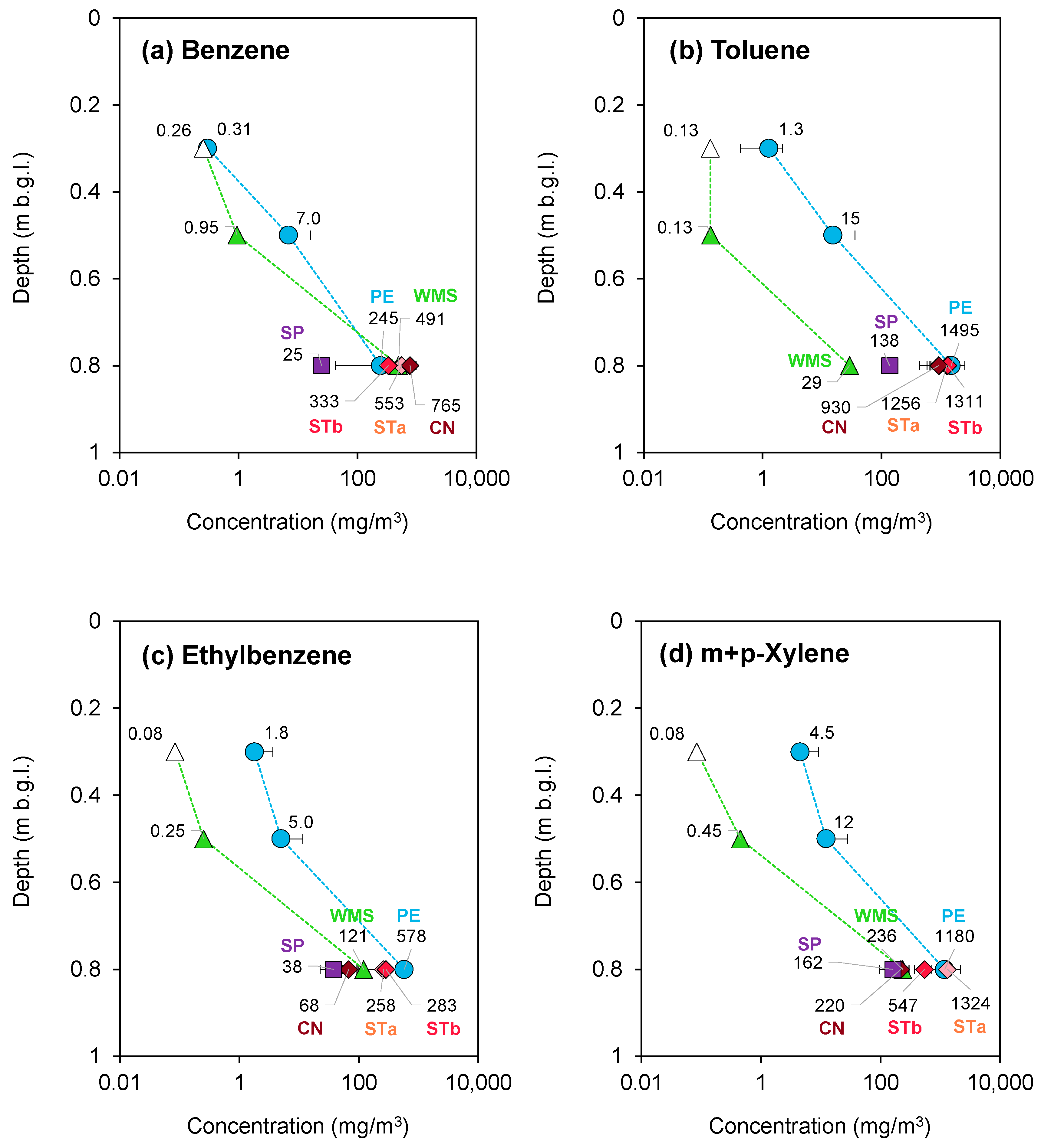
3.1.1. Porto Marghera—August 2020 Campaign

Figure 3 presents a comparison of the average soil gas concentrations of trichloroethene (TCE, Figure 3a) and tetrachloroethene (PCE, Figure 3b) obtained in the first campaign carried out at the Porto Marghera site. The soil gas concentrations were measured using vacuum bottles (VBs) for the active systems and polyethylene (PE) films and Waterloo Membrane Samplers (WMS) for the passive samplers (see Table 1, Figure 1a and SI). For active sampling, four soil gas samples were obtained for each probe investigated during the two-day campaign, with each sampling session lasting approximately 20 min. The PE films were instead exposed for 24 h, while the WMS were exposed for either 4 or 24 h. For additional details, refer to the Supporting Information.

The results reported in the graphs represent the average values from each sampling system over time during the campaign (e.g., active samplings repeated over two days) or at different measurement points in the experimental area (e.g., the average concentrations obtained by active sampling in the two probes SGP01 and SGP02). The error bars indicate the standard deviation of the results obtained. Among the analyzed compounds, only the results for TCE and PCE are presented graphically, as these were the only two compounds, along with hexachlorobutadiene (HCBD), for which monitoring results indicated concentrations above the limit of quantification (LOQ) in at least two systems. However, the results for HCBD are not included, as this campaign only tested 24 h exposure times for PE, which were insufficient for the compound to reach equilibrium conditions. Note that the achieved LOQ for the active sampling was on the order of µg/m³, while for the passive sampling it was on the order of tens of µg/m³. The specific LOQs achieved for each contaminant in each monitoring campaign are reported in the SI.

For this campaign, PE was the only system tested at different depths. Figure 3 shows that for both compounds, an increase in average concentration by approximately a factor of 10 can be observed with an increasing sampling depth. The concentrations of TCE obtained with the passive PE-based samplers were consistent with those measured with the active system (VB) at the same depth. For PCE (Figure 3b), the data obtained with PE showed slightly higher concentrations than those obtained with the active sampling system (VB). However, these concentrations were similar to those obtained with the passive WMS system exposed for 4 h. Additionally, the results obtained with the WMS exposed for 24 h were slightly higher than those obtained with the shorter exposure time (4 h). This could be due to a potential saturation effect of the samplers for longer exposure times, which could result in an underestimation of the actual concentrations detected [17]. Nevertheless, the three different tested systems appear to provide consistent information for the two compounds. When analyzing the results obtained using the different sampling systems, it should be noted that while the study area was relatively small, the systems were not deployed at exactly the same locations. As such, some discrepancies between the different sampling methods may also be partially attributed to spatial variability in contamination levels. In the specific case of Porto Marghera, however, an examination of the concentrations measured at individual sampling points (as reported in the SI) suggests that spatial variability was limited. Indeed, for each compound, concentrations recorded at the same depth were generally within the same order of magnitude.

3.1.2. Porto Marghera—February 2022 Campaign

Figure 4 shows the comparison of the average soil gas concentrations obtained from each sampling system deployed at the specified sampling depth in all the sampling points in the test area over the course of the second campaign at the Porto Marghera site. Active sampling was conducted using vacuum bottles (VBs), while passive sampling employed polyethylene (PE) films and Waterloo Membrane Samplers (WMS) (see Table 1, Figure 1b and Supplementary Information SI). Similar to the first campaign, four soil gas samples were obtained for each probe investigated, with each active sampling session lasting approximately 20 min over the two-day campaign. For passive sampling, different exposure times were tested for the WMS (3–22 h) and PE (3–24 h) samplers. Only the results for TCE and PCE are shown, as these were the only two compounds, along with HCBD, for which monitoring results indicated concentrations above the LOQ for at least two sampling systems.

It can be observed that, despite the different locations of the monitoring points (see Figure 1) and the consequent possible heterogeneity of the contamination, there does not seem to be a trend of increasing concentrations as a function of the different exposure durations tested for PE sampling. These results suggest that for PE, an exposure of 3–6 h was sufficient to achieve equilibrium conditions in line with previous findings [24]. Conversely, it can be observed that the concentrations of PCE estimated by the WMS passive samplers were, on average, higher for shorter exposures. These results suggest that the concentrations obtained by the WMS samplers exposed for 21–24 h may, in fact, underestimate the actual concentrations in soil gas, as the samplers may have reached saturation conditions.

Comparing the results obtained with the different sampling systems, it can also be observed that, unlike the results obtained in the first campaign, in this campaign, the estimated concentrations in soil gas for TCE and PCE with VBs were about ten times lower than those obtained with passive sampling systems. In contrast, the passive sampling results were consistent for PCE (TCE was not detected with the WMS, thus the comparison is not feasible). The differences between active and passive soil gas sampling observed in this campaign may be due to possible surface air permeation into the soil gas sampling probes during active sampling.

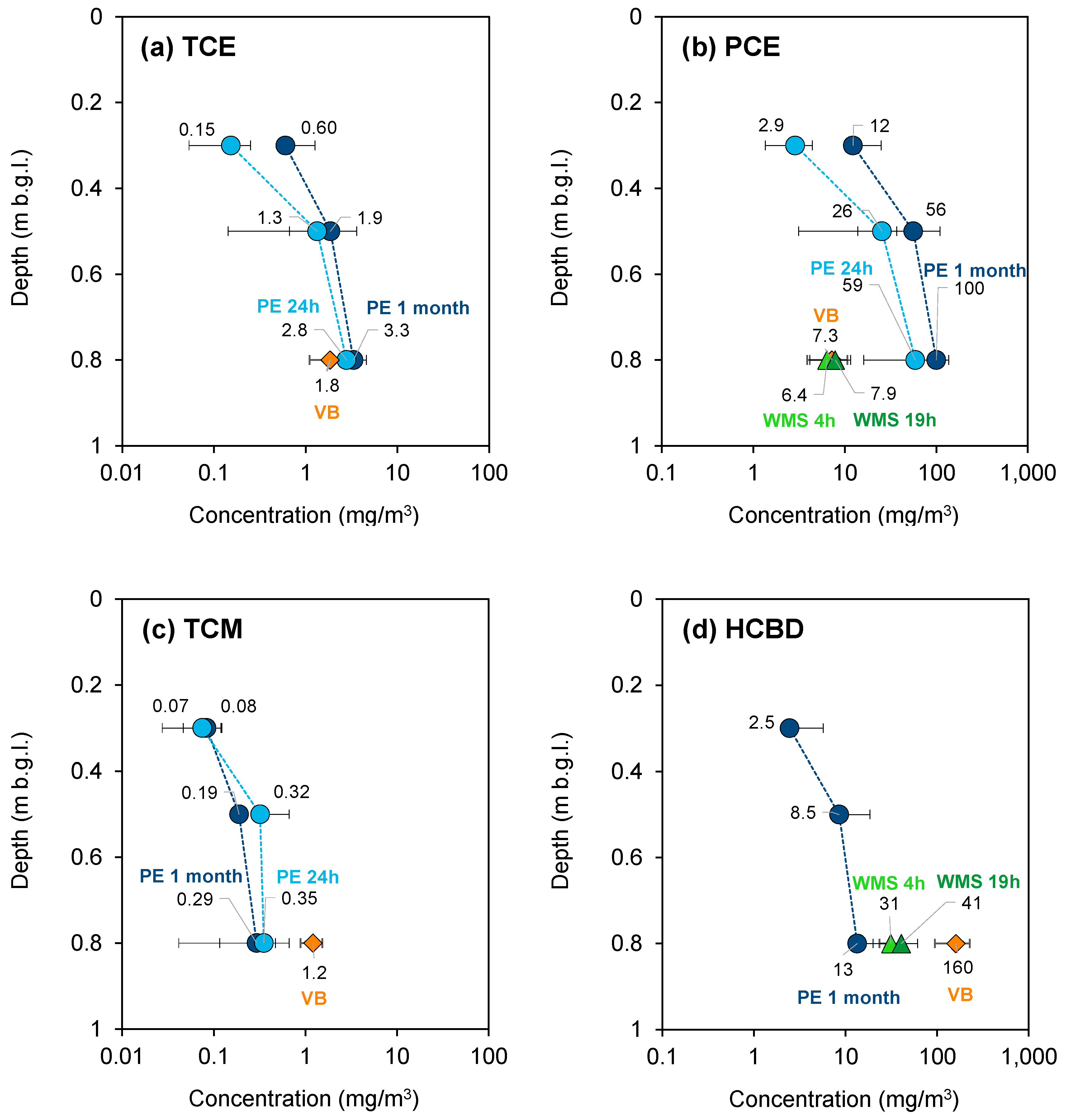
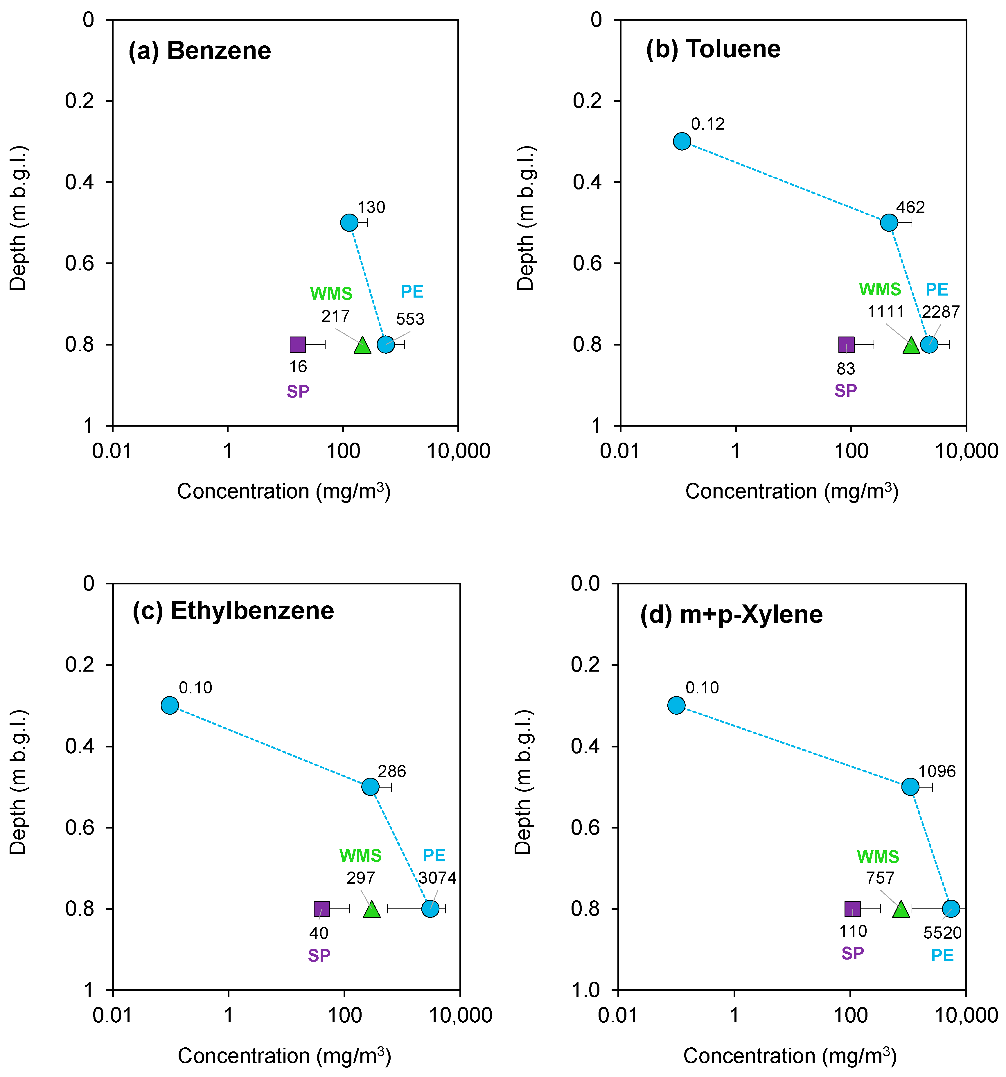
3.1.3. Porto Marghera—September 2022 Campaign

Figure 5 presents a comparison of the average soil gas concentrations obtained from each sampling system deployed at the specified sampling depth in all sampling points within the test area during the third campaign at the Porto Marghera site. Similar to previous campaigns, active sampling was performed using vacuum bottles (VBs), while passive sampling utilized polyethylene (PE) films and Waterloo Membrane Samplers (WMS) (see Table 1, Figure 1c and SI). For active sampling, four soil gas samples were collected from each probe, with each session lasting approximately 20 min. For passive sampling, different exposure times were tested, with 4 h and 19 h for the WMS, and 24 h and 1 month for the PE samplers. The one-month exposure duration for PE was used to monitor HCBD, as a 24 h period was deemed insufficient to achieve equilibrium conditions in previous experiments. Compared to previous campaigns, the results for HCBD and trichloromethane (TCM) are also shown.

It can be observed that the TCE concentrations (Figure 5a) obtained with PE are aligned with those obtained with VBs. The same result was observed in the first campaign. Also, for TCM (Figure 5c), soil gas concentrations obtained with PE are aligned with those determined with the active sampling system, although the average concentration values are slightly lower. Conversely, for PCE (Figure 5b), the data obtained with PE were higher than those obtained with WMS and active sampling methods in both areas, while WMS and active sampling appeared to be consistent. In contrast, the concentration data obtained with PE and WMS for HCBD (Figure 5d) were, on average, approximately one order of magnitude lower than those obtained with the active soil gas survey. These discrepancies can be partly attributed to an insufficient exposure time for PE to reach equilibrium and to the K_PEa coefficient used for this compound, which was derived from the octanol–air partition coefficient by extrapolation of the empirical correlation outside the experimental range [24]. In the case of WMS, this discrepancy can be attributed to the value of the UR_WMS used, which, as previously described, was not included in the list of coefficients defined by the supplier but was extrapolated using the LTPRI method [43]. As discussed earlier, minor discrepancies between sampling systems may also reflect spatial variability within the study area.

3.2. Ferrara Campaigns

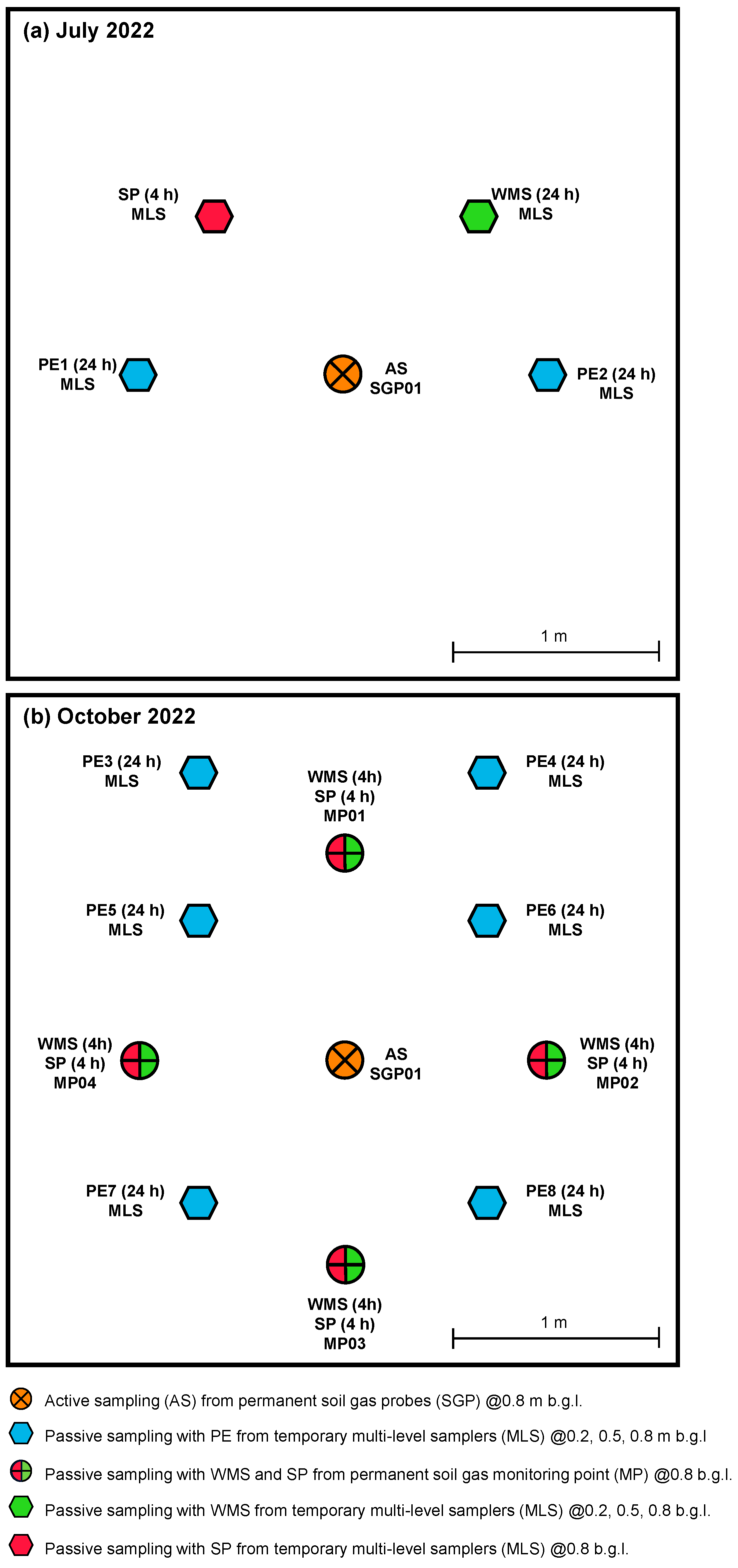
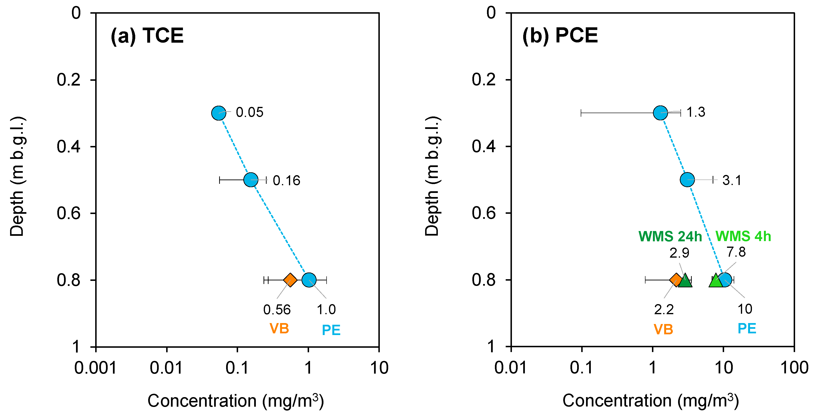
3.2.1. Ferrara—July 2022 Campaign

Figure 6 shows a comparison of the average soil gas concentrations (with the corresponding error bar representing the standard deviation of the results obtained) of BTEX compounds obtained from each sampling system installed in the test area at the indicated sampling depth. In particular, the figures present the results for selected compounds for which the concentrations resulted above the LOQ with at least two systems. Active sampling was conducted using canisters (CNs) and sorbent tubes (STs) while PE films, WMS, and sorbent pens were employed for passive sampling (see Table 1, Figure 2a and Supplementary Information). During the two-day campaign, six soil gas active samplings using sorbent tubes by two different laboratories were carried out (3 samples for each laboratory). The duration of the active sampling with the sorbent tubes was 60 min for one sample and 240 min for the other two. For canisters, two samples were collected, each lasting approximately 240 min. For passive sampling, the exposure time was 24 h for both polyethylene (PE) and Waterloo Membrane Samplers (WMS), while the sorbent pens were exposed for 4 h. PE and WMS were tested at depths of 0.3, 0.5, and 0.8 m below ground level (b.g.l.), while active sampling was conducted at a depth of 0.8 m b.g.l. In the case of concentrations below the LOQ, the LOQ values (indicated by the blank markers) are shown as a reference in the graphs. As previously discussed, the achieved LOQ for the active sampling was on the order of µg/m³, while for the passive sampling it was on the order of tens of µg/m³ (see Supplementary Information).

It can be observed that for BTEX (Figure 6), there is a strong increase in average concentrations (by a factor of approximately 100–1000) with increasing sampling depth. In Figure 6, the comparison of BTEX values obtained at a depth of 0.8 m b.g.l demonstrates a certain degree of variability in the results provided by active sampling systems, even when the same system is utilized (i.e., STa and STb). This variability is observed to be relatively minor for benzene and toluene, whereas it was more pronounced, by a factor of approximately 10, for ethylbenzene and m+p-xylene. It can be observed that the results provided by PE are consistent with those obtained through active sampling. Similarly, WMS yields results that align with those of active sampling and PE for benzene and ethylbenzene, while exhibiting lower values for toluene and, to a lesser extent, for m+p-xylene. SPs exhibited lower values than the other systems tested for most of the compounds. This can partly be attributed to improper fiber exposure (as the fiber was not fully retracted), which was caused by an unsuitable insertion system. As observed in the other case study, another factor to consider when interpreting the differences observed across the various sampling systems is the spatial variability of subsurface contamination. Although the concentrations measured using both PE and active systems at different sampling points were generally within the same order of magnitude (see Supplementary Information), the lower concentrations detected by the sorbent pens could also be partially attributed to lower local contamination at the specific monitoring point.

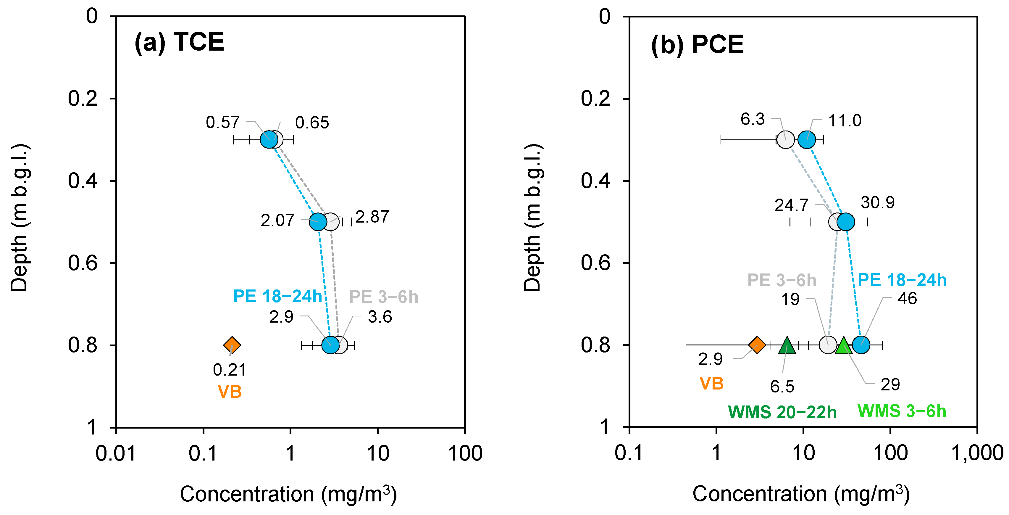
3.2.2. Ferrara—October 2022 Campaign

In the second campaign carried out at the Ferrara site, active sampling was conducted using canisters (CNs) and sorbent tubes (STs) while PE films, WMS, and sorbent pens were employed for passive sampling (see Table 1, Figure 2b and Supplementary Information). During the two-day campaign, six soil gas active samplings using sorbent tubes by two different laboratories were carried out (3 samples for each laboratory). The duration of the active sampling with the sorbent tubes was 60 min for one sample and 240 min for the other two. For canisters, three samples were collected, each lasting approximately 240 min. For passive sampling, the exposure time was 24 h for polyethylene (PE) while the Waterloo Membrane Samplers (WMS) and sorbent pens were exposed for 4 h. PE and WMS were tested at depths of 0.3, 0.5, and 0.8 m b.g.l., while active sampling was conducted at a depth of 0.8 m b.g.l. Figure 7 presents the comparison of the average soil gas concentrations obtained from each passive sampling system installed at the specified sampling depth at all sampling locations within the test area. Active sampling results are not presented here, as all systems used for this campaign consistently provided concentrations below the LOQ (see SI). It is worth noting that the absence of VOCs detected by active sampling can be attributed to potential sampling issues, particularly with respect to soil moisture levels, which were observed to range from 60 to 80 percent depending on the time of active sampling during the two-day campaign. For comparison, data for benzene, toluene, ethylbenzene, and m+p-xylene are presented graphically in Figure 7. Tables S51–S61 in the Supplementary Information show all the values obtained for other compounds as well.

The concentrations obtained with the polyethylene passive samplers were consistently higher than those obtained with the Waterloo Membrane Samplers and sorbent pens. Across the entire area, the WMS produced results consistent with those of the PE for benzene and toluene, but approximately an order of magnitude lower for ethylbenzene and m+p-xylene. The passive SP samplers provided results that were 10–100 times lower than those obtained with PE at a depth of 0.8 m b.g.l. These results, limited to comparisons between passive systems (as a comparison with active sampling systems was not feasible for this campaign), are consistent with those obtained in the previous campaign.

It is worth noting that, compared to the other campaigns, this campaign showed greater spatial variability, with different concentrations detected at the same depth even when using the same technique (e.g., see the results for PE in the Supplementary Information). Therefore, some of the differences observed between the various sampling systems in this case may be attributed to the heterogeneity of the contamination.

4. Conclusions

This work provided valuable insights into the performance and limitations of the various soil gas sampling methods for VOC monitoring at contaminated sites. Given the intrinsic spatial and temporal variability of the soil gas matrix, the results obtained were generally consistent across the different sampling techniques tested. However, uncertainties were identified for each method, highlighting the value of using multiple lines of evidence to achieve a more robust analysis of soil gas concentrations.

Active sampling methods, while typically more expensive, offer the advantage of almost real-time, high-resolution VOC capture and are generally more robust for compounds with lower volatility. The active systems tested in this study (vacuum bottles, sorbent tubes, and canisters) confirmed their overall good performance but also revealed specific challenges. For instance, at the Ferrara site, variability in soil gas concentrations was observed for the sampling point and day, depending on the device or laboratory that performed the analysis. Additionally, lower concentrations of certain compounds were often detected compared to passive samplers, probably because of specific active sampling challenges such as high soil moisture or atmospheric air infiltration. It should also be noted that active sampling systems, by extracting volumes of air from the interstitial gases (ranging from 0.5 L in the case of vacuum bottles to several liters for canisters and sorbent tubes), may slightly alter the subsurface equilibrium. This effect can be particularly relevant in the presence of strong vertical concentration gradients, as observed in the case studies presented in this work.

PE passive samplers provided results consistent with active methods, with average concentrations typically in the same order of magnitude. However, discrepancies were observed for heavier compounds (e.g., hexachlorobutadiene), particularly at shorter exposure times, likely due to slower diffusion of these VOCs through the PE film. Adjustments in exposure times partially resolved these issues. The WMS passive samplers also demonstrated consistency with PE films and active sampling for lighter chlorinated VOCs during shorter exposure campaigns. However, for heavier compounds and BTEX, lower concentrations were typically observed than with active sampling. Sorbent pens, tested only at the second site, showed mixed results; while concentrations of BTEX were significantly lower than those obtained with active sampling, results for chlorinated compounds varied depending on the analyte.

Overall, passive samplers offer several advantages, including lower costs, ease of use, and the ability to achieve greater spatial coverage. Systems like PE and, to a lesser extent, WMS are relatively economical, require no suction equipment, and have minimal shipping and maintenance costs due to their small size and disposability. Unlike active methods, passive samplers avoid short-circuiting effects from atmospheric air infiltration and eliminate the need for line purging or leak testing, simplifying deployment. This also allows detailed vertical and spatial concentration profiling even at shallow depths. Furthermore, direct-push installation allows for denser sampling grids at reduced costs compared to permanent probes. However, limitations remain, including sorbent saturation and equilibrium constraints for heavier compounds. For instance, PE films showed variability in detecting heavier VOCs due to insufficient equilibrium times, while WMS systems may be prone to starvation effects, potentially underestimating soil gas concentrations.

Combining active and passive sampling methods provides a more comprehensive and reliable characterization of soil gas contamination in complex scenarios, especially in heterogeneous subsurface environments with preferential soil gas migration pathways. Passive samplers, in particular, are a valuable tool for identifying contamination sources, offering broader spatial coverage and a more detailed understanding of contamination in environments where active sampling might not be as effective. By integrating both approaches, a more complete and accurate analysis of soil gas contamination can be achieved.

References

1. McHugh, T.E.; De Blanc, P.C.; Pokluda, R.J. Indoor Air as a Source of VOC Contamination in Shallow Soils Below Buildings. Soil Sediment Contam. Int. J. 2006, 15, 103–122. [Google Scholar] [CrossRef]
2. US EPA. Technical Guide for Assessing and Mitigating the Vapor Intrusion Pathway from Subsurface Vapor Sources to Indoor Air. OSWER Publication 9200.2–154. 2015. Available online: https://www.epa.gov/vaporintrusion/technical-guide-assessing-and-mitigating-vapor-intrusion-pathway-subsurface-vapor (accessed on 24 April 2025).
3. Ma, J.; McHugh, T.; Beckley, L.; Lahvis, M.; DeVaull, G.; Jiang, L. Vapor Intrusion Investigations and Decision-Making: A Critical Review. Environ. Sci. Technol. 2020, 54, 7050–7069. [Google Scholar] [CrossRef] [PubMed]
4. ASTM D5314-92e1; ASTM Standard Guide for Soil Gas Monitoring in the Vadose Zone. ASTM International: West Conshohocken, PA, USA, 2006.
5. Verginelli, I.; Pecoraro, R.; Baciocchi, R. Using Dynamic Flux Chambers to Estimate the Natural Attenuation Rates in the Subsurface at Petroleum Contaminated Sites. Sci. Total Environ. 2018, 619–620, 470–479. [Google Scholar] [CrossRef]
6. Verginelli, I.; Baciocchi, R. Refinement of the Gradient Method for the Estimation of Natural Source Zone Depletion at Petroleum Contaminated Sites. J. Contam. Hydrol. 2021, 241, 103807. [Google Scholar] [CrossRef] [PubMed]
7. Yao, Y.; Verginelli, I.; Suuberg, E.M.; Eklund, B. Examining the Use of USEPA’s Generic Attenuation Factor in Determining Groundwater Screening Levels for Vapor Intrusion. Groundw. Monit. Remediat. 2018, 38, 79–89. [Google Scholar] [CrossRef]
8. Verginelli, I.; Yao, Y. A Review of Recent Vapor Intrusion Modeling Work. Groundw. Monit. Remediat. 2021, 41, 138–144. [Google Scholar] [CrossRef]
9. Gorder, K.A.; Dettenmaier, E.M. Portable GC/MS Methods to Evaluate Sources of cVOC Contamination in Indoor Air. Groundw. Monit. Remediat. 2011, 31, 113–119. [Google Scholar] [CrossRef]
10. Steinemann, A. Volatile Emissions from Common Consumer Products. Air Qual. Atmos. Health 2015, 8, 273–281. [Google Scholar] [CrossRef]
11. Geosyntec Scoping Assessment of Soil Vapor Monitoring Protocols for Evaluating Subsurface Vapor Intrusion into Indoor Air 2009. Available online: https://www.geosyntec.com/vapor-intrusion-guidance (accessed on 24 April 2025).
12. CalEPA, (California Environmental Protection Agency Department of Toxic Substances Control) Advisory: Active Soil Gas Investigations. 2015. Available online: https://www.waterboards.ca.gov/rwqcb4/water_issues/programs/ust/docs/VI_ActiveSoilGasAdvisory_FINAL.pdf (accessed on 24 April 2025).
13. API. Collecting and Interpreting Soil Gas Samples from the Vadose Zone: A Practical Strategy for Assessing the Subsurface Vapor-to-Indoor Air Migration Pathway at Petroleum Hydrocarbon Sites; API Publication: Washington, DC, USA, 2005; Available online: https://www.api.org/~/media/files/ehs/clean_water/ground_water_quality/pub4741_vi_assessment_2005.pdf (accessed on 24 April 2025).
14. ITRC. Vapor Intrusion Pathway: A Practical Guideline; VI-1; ITRC: Kansas City, MO, USA, 2007; Available online: https://itrcweb.org/petroleum-vapor-intrusion-2/ (accessed on 24 April 2025).
15. SNPA. Progettazione del Monitoraggio dei Vapori Nei Siti Contaminati. Linee Guida SNPA 15/2018. 2018. Available online: https://www.snpambiente.it/snpa/progettazione-del-monitoraggio-di-vapori-nei-siti-contaminati/ (accessed on 24 April 2025).
16. Cocheo, C.; Boaretto, C.; Pagani, D.; Quaglio, F.; Sacco, P.; Zaratin, L.; Cottica, D. Field Evaluation of Thermal and Chemical Desorption BTEX Radial Diffusive Sampler Radiello® Compared with Active (Pumped) Samplers for Ambient Air Measurements. J. Environ. Monit. 2009, 11, 297–306. [Google Scholar] [CrossRef]
17. McAlary, T.; Wang, X.; Unger, A.; Groenevelt, H.; Górecki, T. Quantitative Passive Soil Vapor Sampling for VOCs- Part 1: Theory. Environ. Sci. Process. Impacts 2014, 16, 482–490. [Google Scholar] [CrossRef]
18. McAlary, T.; Groenevelt, H.; Seethapathy, S.; Sacco, P.; Crump, D.; Tuday, M.; Schumacher, B.; Hayes, H.; Johnson, P.; Górecki, T. Quantitative Passive Soil Vapor Sampling for VOCs—Part 2: Laboratory Experiments. Environ. Sci. Process. Impacts 2014, 16, 491–500. [Google Scholar] [CrossRef] [PubMed]
19. McAlary, T.; Groenevelt, H.; Nicholson, P.; Seethapathy, S.; Sacco, P.; Crump, D.; Tuday, M.; Hayes, H.; Schumacher, B.; Johnson, P.; et al. Quantitative Passive Soil Vapor Sampling for VOCs—Part 3: Field Experiments. Environ. Sci. Process. Impacts 2014, 16, 501–510. [Google Scholar] [CrossRef] [PubMed]
20. McAlary, T.; Groenevelt, H.; Seethapathy, S.; Sacco, P.; Crump, D.; Tuday, M.; Schumacher, B.; Hayes, H.; Johnson, P.; Parker, L.; et al. Quantitative Passive Soil Vapor Sampling for VOCs—Part 4: Flow-through Cell. Environ. Sci. Process. Impacts 2014, 16, 1103–1111. [Google Scholar] [CrossRef]
21. McAlary, T.; Groenevelt, H.; Disher, S.; Arnold, J.; Seethapathy, S.; Sacco, P.; Crump, D.; Schumacher, B.; Hayes, H.; Johnson, P.; et al. Passive Sampling for Volatile Organic Compounds in Indoor Air-Controlled Laboratory Comparison of Four Sampler Types. Environ. Sci. Process. Impacts 2015, 17, 896–905. [Google Scholar] [CrossRef]
22. Hamamin, D.F. Passive Soil Gas Technique for Investigating Soil and Groundwater Plume Emanating from Volatile Organic Hydrocarbon at Bazian Oil Refinery Site. Sci. Total Environ. 2018, 622–623, 1485–1498. [Google Scholar] [CrossRef]
23. Liang, C.; Chang, J.-S.; Chen, T.-W.; Hou, Y. Passive Membrane Sampler for Assessing VOCs Contamination in Unsaturated and Saturated Media. J. Hazard. Mater. 2021, 401, 123387. [Google Scholar] [CrossRef]
24. Gschwend, P.; MacFarlane, J.; Jensen, D.; Soo, J.; Saparbaiuly, G.; Borrelli, R.; Vago, F.; Oldani, A.; Zaninetta, L.; Verginelli, I.; et al. In Situ Equilibrium Polyethylene Passive Sampling of Soil Gas VOC Concentrations: Modeling, Parameter Determinations, and Laboratory Testing. Environ. Sci. Technol. 2022, 56, 7810–7819. [Google Scholar] [CrossRef] [PubMed]
25. Moon, J.-K.; Kim, P.-G.; Lee, K.Y.; Kwon, J.-H.; Hong, Y. Development of an in Situ Equilibrium Polydimethylsiloxane Passive Sampler for Measuring Volatile Organic Compounds in Soil Vapor. Chemosphere 2023, 325, 138419. [Google Scholar] [CrossRef]
26. Kim, P.-G.; Tarafdar, A.; Lee, K.Y.; Kwon, J.-H.; Hong, Y. The Passive Sampler Assisted Human Exposure Risk Characterization for Tetrachloroethene Soil Vapor Intrusion Scenario. Environ. Res. 2023, 238, 117238. [Google Scholar] [CrossRef]
27. Górecki, T.; Namieśnik, J. Passive Sampling. TrAC Trends Anal. Chem. 2002, 21, 276–291. [Google Scholar] [CrossRef]
28. Huang, C.; Shan, W.; Xiao, H. Recent Advances in Passive Air Sampling of Volatile Organic Compounds. Aerosol Air Qual. Res. 2018, 18, 602–622. [Google Scholar] [CrossRef]
29. Brown, R.H.; Charlton, J.; Saunders, K.J. The Development of an Improved Diffusive Sampler. Am. Ind. Hyg. Assoc. J. 1981, 42, 865–869. [Google Scholar] [CrossRef]
30. Fowler, W.K. Fundamentals of Passive Vapor Sampling. American Laboratory 1982, 14, 80–82. [Google Scholar]
31. Seifert, B.; Abraham, H.-J. Use of Passive Samplers for the Determinaton of Gaseous Organic Substances in Indoor Air at Low Concentration Levels. Int. J. Environ. Anal. Chem. 1983, 13, 237–253. [Google Scholar] [CrossRef]
32. Lewis, R.G.; Mulik, J.D.; Coutant, R.W.; Wooten, G.W.; McMillin, C.R. Thermally Desorbable Passive Sampling Device for Volatile Organic Chemicals in Ambient Air. Anal. Chem. 1985, 57, 214–219. [Google Scholar] [CrossRef]
33. Zabiegała, B.; Kot-Wasik, A.; Urbanowicz, M.; Namieśnik, J. Passive Sampling as a Tool for Obtaining Reliable Analytical Information in Environmental Quality Monitoring. Anal. Bioanal. Chem. 2010, 396, 273–296. [Google Scholar] [CrossRef]
34. Borrelli, R.; Tcaciuc, A.P.; Verginelli, I.; Baciocchi, R.; Guzzella, L.; Cesti, P.; Zaninetta, L.; Gschwend, P.M. Performance of Passive Sampling with Low-Density Polyethylene Membranes for the Estimation of Freely Dissolved DDx Concentrations in Lake Environments. Chemosphere 2018, 200, 227–236. [Google Scholar] [CrossRef]
35. Hodny, J.W.; Whetzel, J.E., Jr.; Anderson, H.S., II. Quantitative Passive Soil Gas and Air Sampling in Vapor Intrusion Investigations. In Proceedings of the AW&MA Vapor Intrusion 2009 Conference, San Diego, CA, USA, 27–30 January 2009. [Google Scholar]
36. Clarke, J.N.; Goodwin, D.F.; O’Neill, H.; Odencrantz, J.E. Application of Passive Soil Gas Technology to Determine the Source and Extent of a PCE Groundwater Plume in an Urban Environment. Remediat. J. 2008, 18, 55–62. [Google Scholar] [CrossRef]
37. Seethapathy, S.; Górecki, T. Applications of Polydimethylsiloxane in Analytical Chemistry: A Review. Anal. Chim. Acta 2012, 750, 48–62. [Google Scholar] [CrossRef]
38. Grosse, D.; McKernan, J. Passive Samplers for Investigations of Air Quality: Method Description, Implementation, and Comparison to Alternative Sampling Methods; U.S. Environmental Protection Agency: Washington, DC, USA, 2014.
39. Namiesnik, J.; Gorecki, T.; Kozlowski, E.; Torres, L.; Mathieu, J. Passive Dosimeters—An Approach to Atmospheric Pollutants Analysis. Sci. Total Environ. 1984, 38, 225–258. [Google Scholar] [CrossRef]
40. Feigley, C.E.; Lee, B.M. Determination of Sampling Rates of Passive Samplers for Organic Vapors Based on Estimated Diffusion Coefficients. Am. Ind. Hyg. Assoc. J. 1987, 48, 873–876. [Google Scholar] [CrossRef]
41. Namieśnik, J.; Zabiegała, B.; Kot-Wasik, A.; Partyka, M.; Wasik, A. Passive Sampling and/or Extraction Techniques in Environmental Analysis: A Review. Anal. Bioanal. Chem. 2005, 381, 279–301. [Google Scholar] [CrossRef] [PubMed]
42. Seethapathy, S.; Górecki, T. Polydimethylsiloxane-Based Permeation Passive Air Sampler. Part II: Effect of Temperature and Humidity on the Calibration Constants. J. Chromatogr. A 2010, 1217, 7907–7913. [Google Scholar] [CrossRef] [PubMed]
43. Seethapathy, S.; Górecki, T. Polydimethylsiloxane-Based Permeation Passive Air Sampler. Part I: Calibration Constants and Their Relation to Retention Indices of the Analytes. J. Chromatogr. A 2011, 1218, 143–155. [Google Scholar] [CrossRef]
44. SIREM Instructions for Soil Gas Sampling with WMS-LUTM Samplers. 2016. Available online: https://www.siremlab.com/wp-content/uploads/2021/02/WMS-SOP-passive-soil-gas-sampling.pdf (accessed on 24 April 2025).
45. U.S. Environmental Protection Agency (EPA). Compendium of Methods for the Determination of Toxic Organic Compounds in Ambient Air—Method TO-15: Determination of Volatile Organic Compounds (VOCs) in Air Collected in Specially-Prepared Canisters and Analyzed by Gas Chromatography/Mass Spectrometry (GC/MS); EPA/625/R-96/010b; Center for Environmental Research Information, Office of Research and Development, U.S. EPA: Cincinnati, OH, USA, 1999.
46. Ente Nazionale Italiano di Unificazione (UNI). UNI CEN/TS 13649: Stationary Source Emissions—Determination of the Mass Concentration of Individual Gaseous Organic Compounds—Adsorption on Solid Sorbent and Thermal Desorption/Gas Chromatographic Analysis; UNI: Milan, Italy, 2002. [Google Scholar]
Figure 1. Schematic layout of the monitoring points and systems for the Porto Marghera campaigns conducted during (a) August 2020, (b) February 2022, and (c) September 2022. PE: Low-density polyethylene films; WMS: Waterloo Membrane SamplerTM. Note that the number after PE refers to the ID assigned to each monitoring point.
Environments 12 00141 g001
Figure 2. Schematic layout of the monitoring points and systems for the Ferrara campaigns conducted during (a) July 2022 and (b) October 2022. PE: Low-density polyethylene films; WMS: Waterloo Membrane SamplerTM. Note that the number after PE refers to the ID assigned to each monitoring point.
Environments 12 00141 g002
Figure 3. Average concentration values obtained for (a) trichloroethene (TCE) and (b) tetrachloroethene (PCE) with different active (vacuum bottles, VBs) and passive (Waterloo Membrane Samplers, WMS and polyethylene films, PE) soil gas sampling systems in the August 2020 test for the entire experimentation area at Porto Marghera.
Environments 12 00141 g003
Figure 4. Average concentration values obtained for (a) trichloroethene (TCE) and (b) tetrachloroethene (PCE) with different active (vacuum bottles, VBs) and passive (Waterloo Membrane Samplers, WMS and polyethylene films, PE) soil gas sampling systems in the February 2022 test for the entire experimentation area at Porto Marghera.
Environments 12 00141 g004
Figure 5. Average concentration values obtained for (a) trichloroethene (TCE), (b) tetrachloroethene (PCE), (c) trichloromethane (TCM), and (d) hexachlorobutadiene (HCBD) with different active (vacuum bottles, VBs) and passive (Waterloo Membrane Samplers, WMS and polyethylene films, PE) soil gas sampling systems in the September 2022 test for the entire experimentation area at Porto Marghera.
Environments 12 00141 g005
Figure 6. Average concentration values obtained for BTEX with different active (sorbent tubes, STa, sorbent tubes analyzed by an external laboratory, STb, and canisters, CNs) and passive (Waterloo Membrane Samplers, WMS, polyethylene films, PE and sorbent pens, SPs) soil gas sampling systems in the July 2022 test for the entire experimentation area at Ferrara.
Environments 12 00141 g006
Figure 7. Average concentration values obtained for BTEX with different passive (Waterloo Membrane Samplers, WMS, polyethylene films, PE, and sorbent pens, SPs) soil gas sampling systems in the October 2022 test for the entire experimentation area at Ferrara.
Environments 12 00141 g007